Electrical Generation and Distribution Systems and Power Quality Disturbances Part 9 pptx
Bạn đang xem bản rút gọn của tài liệu. Xem và tải ngay bản đầy đủ của tài liệu tại đây (645.45 KB, 20 trang )
Power Quality and Voltage Sag Indices in Electrical Power Systems
147
severity. Observing the graph shown in Figure 4, there are 5 events per year where the
voltage drops below 40% of nominal Voltage for 0.1 s or longer. Equally there are 5 events
per year where the voltage drops below 70% magnitude and 250 ms duration.
0s 0.2s 0.4s 0.6s 0.8s
90%
80%
70%
60%
50%
40%
30%
20%
10%
Sag duration (s)
5
10
25
15
20
device A
device B
Voltage (pu)
N
u
m
b
e
r
o
f
E
v
e
n
t
s
Fig. 4. Voltage sag co-ordination chart
The advantage of this method is that equipment behavior can be directly compared with
system performance, for a wide range of equipment. The disadvantage of the method is that
a two-dimensional function is needed to describe the site. For comparison of different sites a
smaller number of indices would be preferred.
3.4.2 Calculation methods
a. Method used by Detroit Edison
The method calculates a “sag score” from the voltage magnitudes in the three phases (Sabin,
2000).
1
3
abc
VVV
S
++
=−
(6)
This sag score is equal to the average voltage drop in the three phases. The larger the sag
score, the more severe the event is considered to be.
b. Method proposed by Thallam
A number of site indices can be calculated from the “voltage sag energy” (Thallam, 2000).
The “Voltage Sag Energy Index” (VSEI) is the sum of the voltage sag energies for all events
measured at a given site during a given period:
_VS i
i
VSEI =Ε
(7)
The “Average Voltage Sag Energy Index” (AVSEI) is the average of the voltage sag energies
for all events measured at a given site during a given period:
_
1
1
N
VS i
i
AVSEI
N
=
=Ε
(8)
Electrical Generation and Distribution Systems and Power Quality Disturbances
148
A sensitive setting will result in a large number of shallow events (with a low voltage sag
energy) and this in a lower value for AVSEI.
The sag event frequency index at a particular location and period is suggested as the
number of qualified sag events at a location and period (Thallam & Koellner, 2003).
The System sag count index is the total number of qualified voltage sag events over the
number of monitor locations. By the expression qualifying events, it implies a voltage less
than 90%, with event duration limited to 15 cycles and energy greater or equal to 100.
3.4.3 Non-rectangular events
Non-rectangular events are events in which the voltage magnitude varies significantly
during the event. A method to include non-rectangular events in the voltage-sag
coordination chart is also applicable according to the IEEE defined standard (IEEE Std.493,
1997). Alternatively, the function value can be defined as the number of times per year that
the RMS voltage is less than the given magnitude for longer than the given duration.
EPRI-Electrotek mentions that each phase of each ms variation measurement may contain
multiple components (Thallam, 2000). Consequently, these phase rectangular voltage sag
measurements are easily characterized with respect to magnitude and duration.
Approximately 10% of the events are non-rectangular. These events are much more difficult
to characterize because no single magnitude-duration pair completely represent the phase
measurement.
The method suggested for calculating the indices used by EPRI-Electrotek is called the
''Specified Voltage'' method. This method designates the duration as the period of time that
the rms voltage exceeds a specified threshold voltage level used to characterize the
disturbance.’ The consequence of this method is that an event may have a different duration
when being assessed at different voltage thresholds as shown in Figure 5.
Measurement
Event #1
0
20
40
60
80
100
120
140
0.000 0.167 0.333 0.500 0.667 0.833 1.000 1.167 1.333 1.500 1.667
Time (seconds)
%Volts
T
80%
T
50%
T
10%
Fig. 5. Illustration of "specified voltage" characterization
Most of the single site indices relate the magnitude and duration of the sag and the number
of events. These events can be grouped in order to make their counting easier and more
Power Quality and Voltage Sag Indices in Electrical Power Systems
149
practical. Power quality surveys in the past have just referred to the number of voltage sags
per year for a given site. This value could include minor events, which do not affect any
equipment.
The Canadian Electrical Association recommends tracking 4 indices for sag magnitudes
(referring to the remaining voltage), of 85%, 70%, 40% and 1%. The latter refers to
interruptions rather than sags.
ESKOM (South African Utility), groups voltage sags into five classes (Sabin, 2000):
class Y: 80% – 90% magnitude, 20 ms - 3 sec duration
class X: 40% - 80% magnitude, 20 ms - l50 ms duration
class S: 40% - 80% magnitude, 150 ms - 600 ms duration
class T: 0 - 40% magnitude, 20 ms - 600 ms duration
class Z: 0 – 80% magnitude, 600 ms - 3 sec duration
EPRl -Electrotek suggests the following five magnitudes and three duration ranges to
characterize voltage thresholds:
a. RMS variation Frequency for voltage threshold X: with X=90%, 80%, 70%, 50%, 10%:
the number of events per year with magnitude below X, and duration between 0.5 cycle
and 60 sec.
b. Instantaneous RMS variation Frequency for voltage threshold X: with X=90%, 80%,
70%, 50%: the number of events per year with magnitude below X, and duration
between 0.5 cycle and 0.5 sec.
c. Momentary RMS variation Frequency for voltage threshold X: with X=90%, 80%, 70%,
50%: the number of events per year with magnitude below X, and duration between 0.5
sec and 3 sec.
d. Momentary RMS variation Frequency for voltage threshold I0%: the number of events
per year with a magnitude below 10%, and a duration between 0.5 cycle and 3 sec.
e. Temporary RMS variation Frequency for voltage threshold X: with X=90%, 8070, 70%,
50%, I0%: the number of events per year with magnitude below X, and duration
between 3 sec. and 60 sec.
The duration ranges are based on the definition of instantaneous, momentary and
temporary, as specified by IEEE (IEEE Std. 1159, 1995).
3.5 System indices
System Indices are typically a weighted average of the single-site indices obtained for all or
a number of sites within the system. The difficulty lies in the determination of the weighting
factors. In order to assess any indices for the system, first monitoring of the quality of
supply must take place. When the Electric Power Research Institute (EPRI)-Distribution
Power Quality (DPQ) program placed monitoring equipment on one hundred feeders, these
feeders needed to adequately represent the range of characteristics seen on distribution
systems. This required the researchers to use a controlled selection process to ensure that
both common and uncommon characteristics of the national distribution systems were well
represented in the study sample. Thus a level of randomness is required. Many devices are
susceptible to only the magnitude of the variation. Others are susceptible to the
combination of magnitude and durationOne consideration in establishing a voltage sag
index is that the less expensive a measuring device is, the more likely it will be applied at
many locations, more completely representing the voltage quality electricity users are
experiencing.
Electrical Generation and Distribution Systems and Power Quality Disturbances
150
With this consideration in mind, sag monitoring devices are generally classified into less
expensive devices that can monitor the gross limits of the voltage sag, and more expensive
devices that can sample finer detail such as the voltage-time area and other features that
more fully characterize the sag.
The sag limit device senses the depth, of the voltage sag. The sag area device can sample the
sag in sufficient detail to plot the time profile of the sag. With this detail it could give a
much more accurate picture of the total sag area, in volt-seconds, as well as the gross limits;
the retained voltage, V
r
, is also shown.
The developed RMS variation indices proposed by EPRI-Electrotek, are designed to aid in
the assessment of service quality for a specified circuit area. The indices are defined such
that they may be applied to systems of varying size (Bollen, 2001).Values can be calculated
for various parts of the distribution system and compared to values calculated for the entire
system.
Accordingly, the four indices presented assess RMS variation magnitude and the
combination of magnitude and duration.
a. System Average RMS (Variation) Frequency Index
voltage
( SARFI
x
)
SARFI
x
represents the average number of specified rms variation measurement events
that occurred over the assessment period per customer served, where the specified
disturbances are those with a magnitude less than x for sags or a magnitude greater than x
for swells. Notice that SARFI is defined with respect to the voltage threshold ‘x’ (Sabin,
2000).
i
x
T
N
SARFI
N
=
(9)
where
x = percentage of nominal rms voltage threshold; possible values - 140, 120, 110, 90, 80, 70,
50, and 10
N
i
= number of customers experiencing short-duration voltage deviations with magnitudes
above x% for x >100 or below x% for x <100 due to measurement event i
N
T
=number of customers served from the section of the system to be assessed
b. System Instantaneous Average RMS (Variation) frequency Index
voltage
( SIARFI
x
)
SIARFI
x
represents the average number of specified instantaneous rms variation
measurement events that occurred over the assessment period per customer served. The
specified disturbances are those with a magnitude less than x for sags or a magnitude
greater than x for swells and duration in the range of 0.5 - 30 cycles.
i
x
T
NI
SIARFI
N
=
(10)
Where:
x = percentage of nominal rms voltage threshold; possible values - 140, 120, 110, 90, 80, 70,
and 50
NI
i
= number of customers experiencing instantaneous voltage deviations with magnitudes
above x% For x>100 or below x% for x <100 due to measurement event i
Power Quality and Voltage Sag Indices in Electrical Power Systems
151
Notice that SIARFI
x
is not defined for a threshold value of x = 10%. This is because IEEE Std.
1159, 1995, does not define an instantaneous duration category for interruptions.
c. System Momentary Average RMS (Variation) Frequency Index
vortage
(SMARFIx)
In the same way that SIARFlx is defined for instantaneous variations, SMARFlx is defined
for variations having a duration in the range of 30 cycles to 3 seconds for sags and swells,
and in the range of 0.5 cycles to 3 seconds for interruptions.
i
x
T
NM
SMARFI
N
=
(11)
x = percentage of nominal rms voltage threshold; possible values - 140, 120, 110, 90, 80, 70,
50, and 10
NM =number of customers experiencing momentary voltage deviations with magnitudes
above X% for X >100 or below X% for X <100 due to measurement event i.
d. System Temporary Average RMS (Variation) Frequency Index
vortage
( STARFI
x
)
STARFI
x
is defined for temporary variations, which have a duration in the range of 3 - 60
seconds.
i
x
T
NT
STARFI
N
=
(12)
x = percentage of nominal rms voltage threshold; possible values - 140, 120, 110, 90, 80, 70,
50, and 10.
NT
i
= number of customers experiencing temporary voltage deviations with magnitudes
above x% for x >100 or below x% for x <100 due to measurement event i.
As power networks become more interconnected and complex to analyse, the need for
power quality indices to be easily assessable, and representative of the disturbance they
characterise with minimum parameters, arises. This section has presented the various
Voltage sag indices available in literature. Most of these indices are characterized through
the sag duration and magnitude. To demonstrate the theory of equipment compatibility,
with the use of the System Average RMS Variation Frequency Index, various power
acceptability curves were used.
Electricity distribution companies need to assess the quality of service provided to
customers. Hence, a common index terminology for discussion and contracting is useful.
Future voltage sag indices need to be adjustable and adaptable to incorporate future
changes in technology and system parameters. This would enable implementation of indices
into the next generation of power system planning software.
4. Voltage sag mathematical indices
In this section of the chapter, the mathematical formulation of two voltage sag indices ( ξ
and ζ
1,2
) is introduced as well as the results of the investigation towards their accuracy
establishment. The Mathematical equations describing the development of a Combined
Voltage Index (CVI) are also presented as well as the results obtained by the verification
process. The index supervises the power quality of a system, through characterising voltage
Electrical Generation and Distribution Systems and Power Quality Disturbances
152
sags. The voltage sags are caused by an increase in reactive demand due to induction motor
starting.
A feeder can be modeled by an equivalent two-port network, as shown in Figure 6.
The sending end voltage and current of the system can be represented by equations 13 and 14.
ss rr r
UAUBI
δδ
∠= ∠+
(13)
srrr
ICU DI
δ
=∠+
(14)
Where U
s
is the sending end voltage, I
s
the sending end current, U
r
the receiving end
voltage, I
r
the receiving end current, δ
s
the sending end voltage angle, δ
r
the receiving end
voltage angle, and A,B,C, D are the two port network constants. For a short length line,
corresponding to distribution network, the two port network parameters can be
approximated as: A=D=1, B= Z
θ
∠ , C=0.Where Z is the transmission line impedance vector
magnitude, and θ the transmission line impedance vector angle.
E
θ
∠Z
sUs
δ
∠ rUr
δ
∠
Is Ir
Load
Fig. 6. The equivalent two port network model.
The line power flow, for the active power at the sending and receiving end of the line, can be
described by (15) and (16).
()
2
()
ssr
ssr
UUU
PCos Cos
ZZ
θθδδ
=−+−
(15)
()
2
()
r
UsUr Ur
PCosrsCos
ZZ
θδ δ θ
=+−−
(16)
4.1 ‘ζ’ index
If the index ζ signifies the voltage magnitude during the sag as a per unit function of the
sending voltage (U
r
=ζU
s
), and is substituted in equation 16, equation 17 yields (Polycarpou
& Nouri, 2005).
()
()
2
2
() 0
s
s
rs r
U
U
Cos Cos P
ZZ
ζ
ζ
θδ δ θ
+− − −=
(17)
Thus the solution of the second order equation, resulting from (17), can be calculated using
equation (18).
()()
1
2
2
2
1,2
4
2
r
rs rs
s
ZPCos
Cos Cos
U
Cos
θ
θδ δ θδ δ
ζ
θ
+− ± +− −
=
(18)
Power Quality and Voltage Sag Indices in Electrical Power Systems
153
Equation 18 provides a tool to calculate the voltage sag ,as a per unit value of the sending
end voltage, through angles and power demand.
However, since the equation is obtained through a quadratic equation, it has two solutions.
ζ
1
will be valid for a specific range of parameters. In the same way ζ
2
will be valid for a
different range of parameters. The validity of the two solutions, ζ
1
and ζ
2
, with the use of
various line X/R ratios is investigated in (Nouri et al., 2006). X/R ratio varies from
Distribution to Transmission according to the cables used for the corresponding voltages.
Typical values of X/R ratio are: for a 33kV overhead line -1.4, for a 132kV overhead line -2.4,
for a 275kV overhead line -8.5, for a 400kV overhead line -15. A distribution line example is
the IEEE34, 24.9kV overhead line with X/R ratio of 0.441.
According to the parameters either ζ
1
or ζ
2
will be the correct answer which
should match
the receiving end voltage.
The point of intersection of U
r
with ζ
1
and ζ
2
, occurs when
()
12
cos
ζ
ζθ
−
is equal to zero,
when both solutions are identical. However, in practice a gap develops when both solutions
approach the Ur axis, where none of the two solutions accurately represent the receiving
voltage Ur, as seen in Figure 7.
Ur
practical
practical
Gap
1
ζ
2
ζ
Fig. 7. Developed gap of inaccuracy
The distance between the two curves at the point of the gap can be defined by equation 19.
()
1
2
2
2
12
4
r
rs
s
ZPCos
Cos
U
Cos
θ
θδ δ
ζζ
θ
+− −
−=
(19)
In order to fully investigate the range of accuracy of the two solutions, X/R ratio values of 1
to 15 are used for the line impedance. Since the receiving end power varies according to the
load, five loading conditions are used in the investigation. Each loading consists of
induction motors. The loads are switched in the system one by one to create the effect of
supplying minimum load (one motor) and maximum load (five motors).
Using MathCad, the value of
()
12
cos
ζ
ζθ
−
is calculated for five different loadings and
each X/R ratio, starting from one up to fifteen in steps of one. The results can be seen in
Figure 8 (Nouri et al., 2006).
Electrical Generation and Distribution Systems and Power Quality Disturbances
154
0
0.1
0.2
0.3
0.4
0.5
0.6
0.7
0246810121416
XR ratio
()
θζζ
cos21
minimum
loading
maximum
loading
|
Fig. 8. Mathematical results obtained for
()
12
cos
ζζ
θ
−
It can be observed from Figure 8, that the minimum values of
()
12
cos
ζζ
θ
− occur within
X/R ratio values of 3 to 8, for all test cases. Therefore during those points, the gap of
inaccuracy for the index can be expected for the two solutions. Taking under consideration
Figure 7, solution ζ
1
should cover the ranges less than three and solution ζ
2
should cover
X/R greater than eight. Between those X/R values the gap position varies according to the
loading and the X/R ratio of the line, thus it cannot be generalized. The accuracy of the
defined location of the gap is and verified through application on a two-bus system
within Power system Computer Aided Design software. The resulting data for a test
system of X/R ratio equal to five, shown in Figure 9, verifies the mathematical theory
concerning the gap.
0
0.2
0.4
0.6
0.8
1
1.2
1.4
1.6
1.8
0123456
Loading
Voltage pu
1
ζ
2
ζ
r
U
Fig. 9. ζ
1
,
ζ
2
and U
r
for line X/R ratio of five
As shown in Figure 9, the plot of ζ
1
has a negative slope until loading two, and then it
becomes positive. Whereas the plot of ζ
2
has a positive slope for the initial loadings and
becomes negative when the third load is switched in.
Throughout the investigation of various X/R ratios a pattern was established regarding the
slope of ζ
1
and ζ
2
. When the slope of ζ
1
is negative it is the accurate solution. When
()
12
cos
ζζ
θ
− reaches minimum, ζ
1
deviates and ζ
2
becomes the correct answer with
Power Quality and Voltage Sag Indices in Electrical Power Systems
155
negative slope. Thus their slope is directly related to the minimum value of
()
12
cos
ζζ
θ
−
and to the accuracy of each solution. The relationship between the slope of ζ
1
and ζ
2
with
the index accuracy and choice of solution is described by equation 20. The value of ‘i’ is 1for
ζ
1
or 2 for ζ
2.
()
0
i
i valid
dLoading
ζ
ζ
∂
∀<
=
(20)
4.2 Combined voltage index
If ξ signifies the voltage magnitude during the sag as a per unit function of the sending
voltage (U
r
= ξ U
s
), and is substituted in equation 15, equation 21 yields.
2
()
s
s
sr
ZP
Cos
U
Cos
θ
ξ
θδ δ
−
=
+−
(21)
ξ and ζ
1,2
signify the voltage magnitude during the sag as a per unit function of the sending
voltage. When the two equations are combined, the resulting Combined Voltage Index
(CVI), described by equation 22 features improved accuracy (Polycarpou & Nouri,2005). The
value of CVI is the value of the receiving end voltage of the system power line.
1
a
CVI
a
ξζ
+
=
+
(22)
Where ‘a’ is the value of the scaling factor (Polycarpou & Nouri, 2009) and is defined as
shown in equation 23.
2
1
11
1
2
n
l
hl wl wl hl
a
nkl
=
+−− + −
=
(23)
Where:
()
cos
rs
w
θδ δ
=+−
()
cos
sr
j
θδ δ
=+−
cos
k
θ
=
2
4
r
s
ZP K
h
U
=
and n= Number of loads supplied.
For simplicity, the value of scaling factor setting is 1.6 for the entire range of line X/R ratios
investigated in the next sections of the chapter. Equations 18, 21 and 22 provide a tool to
calculate the load voltage, as a per unit value of the sending end voltage. The equations are
functions of receiving end variables such as the the receiving end voltage angle, δ
r,
and the
receiving end power P
r
. The receiving end power can be described by
2
cos
rs
PPIZ
θ
=− .
The angle δ
r
of the receiving end voltage
can be represented by sending end quantities
through equation 24 (Nouri & Polycarpou, 2005).
Electrical Generation and Distribution Systems and Power Quality Disturbances
156
sin( ) sin( )
tan
cos( ) cos( )
ss
r
ss
UZIi
a
UZIi
δθ
δ
δθ
−+
=
−+
(24)
Assuming the presence of an infinite bus at the sending end, equation 24 can be reduced to
equation 25.
sin( )
tan
cos( ) 1
r
ZI i
a
ZI i
θ
δ
θ
+
=
+−
(25)
4.2.1 Combined voltage index accuracy investigation
Most distribution power system loads have a power factor of 0.9 to 1. Industrial companies
have to keep their power factor within limits defined by the regulatory authorities, or apply
power factor correction techniques, or suffer financial penalties. In order to cover a wider
area of investigation it is decided to simulate loads of power factor 0.8 to 0.99.
The relationship between the power factor and the X/R ratio of a load is: X/R ratio = tan
θ
,
where
1
cos
pf
θ
−
= .
In order to achieve the load X/R ratio variation the circuit model of the double cage
induction motor, used within the PSCAD environment, is considered. The Sqc100 Motor
circuit diagram is shown in Figure 10 (Polycarpou &Nouri, 2002).
Zs
Xm
Xmr
Rr1
Rr2
Xr1
Fig. 10. The Double cage Induction motor model circuit diagram
The motor circuit parameters are:
Slip: 0.02, Stator resistance(Rs) 2.079 pu, First cage resistance(Rr1) 0.009 pu, Second cage
resistance(Rr2)0.012 pu, Stator reactance (Xs)0.009 pu, Magnetizing reactance (Xm) 3.86 pu
Rotor mutual reactance (Xmr) 0.19 pu, First cage reactance (Xr1)0.09 pu
The resistance of the stator winding is varied in order to achieve the required power factor
and X/R ratio. Load X/R ratios of 0.1 to 0.75 are investigated. Two distribution line X/R
ratios are used in the investigation in order to observe the accuracy of the index while
varying both load as well as line X/R ratio for distribution system lines. The line X/R ratios
are 0.12087, and 1. The amount of loading is varied through introducing five identical
motors for each investigated case. The results of this investigation are presented in the
following subsections.
a. Distribution Line X/R ratio is 0.120817
The per unit receiving voltage, obtained with variation of the load X/R ratio while line X/R
ratio is 0.120817, can be seen in Figure 11. M
1
Signifies the minimum loading with the first
motor being switched in. As any switched in motor reaches rated speed, the next load is
switched in the system. M
5
corresponds to the Maximum loading with the fifth motor being
Power Quality and Voltage Sag Indices in Electrical Power Systems
157
switched in while the previous four are in steady state operation. The Combined Voltage
Index (CVI) deviation corresponding to this scenario can be seen in Figure 12.
0.86
0.88
0.9
0.92
0.94
0.96
0.98
1
0 0.1 0.2 0.3 0.4 0.5 0.6 0.7 0.8
Load X/R
U
r
(pu)
M
5
M
4
M
3
M
2
M
1
Fig. 11. U
r
for various Load X/R ratios and loadings whilst Line X/R is 0.120817
0
0.001
0.002
0.003
0.004
0.005
0.006
0.007
0.008
0 0.1 0.2 0.3 0.4 0.5 0.6 0.7 0.8
Load X/R
CVI Dev
M
1
M
2
M
3
M
4
M
5
Fig. 12. CVI deviation for load X/R variation whilst line X/R=0.120817
Observing the figures above it can be concluded that as loading levels (M
1
to M
5
) and X/R
ratio increases, the receiving end voltage naturally decreases. This is due to the voltage drop
occurring on the impedance of the transmission line. The accuracy of the proposed index is
well within acceptable limits(0.7% in the worst case). Thus for line X/R ratio of 0.120817 the
index is capable of calculating the receiving end voltage for variation of load X/R ratio.
b. Distribution Line X/R ratio is 1
The resulting receiving end voltage, obtained through variation of the load X/R ratio for the
specific line X/R ratio can be seen in Figure 13.
Electrical Generation and Distribution Systems and Power Quality Disturbances
158
0.8
0.82
0.84
0.86
0.88
0.9
0.92
0.94
0.96
0.98
1
0 0.1 0.2 0.3 0.4 0.5 0.6 0.7 0.8
Load X/R
Ur(pu)
M
5
M
4
M
3
M
2
M
1
Fig. 13. U
r
for load X/R variation whilst line X/R=1
Comparing Figure 11 to Figure 13, it is concluded that as the X/R ratio of the line increases,
any load increment has more severe impact on the receiving end voltage due to the
impedance magnitude of the line. The CVI deviation corresponding to this investigation
case can be seen in Figure 14.
0
0.005
0.01
0.015
0.02
0.025
0.03
0 0.1 0.2 0.3 0.4 0.5 0.6 0.7 0.8
Load X/R
CVI Dev
M
1
M
2
M
3
M
4
M
5
Fig. 14. CVI deviation for load X/R variation whilst line X/R=1
As the X/R ratio of the line increases the index accuracy did not decrease homogeneously.
Between the values of 0.3 and 0.5 for load X/R an area of decreased inaccuracy can be
observed. This is due to the scaling factor setting being 1.6 for the entire range of line X/R
ratios investigated. The accuracy of the index is within acceptable margins as the largest
deviation is within 2.5% (Polycarpou & Nouri, 2009). The index is within acceptable
accuracy limits.
Power Quality and Voltage Sag Indices in Electrical Power Systems
159
5. Conclusion
The first part of this chapter presents various statistical voltage sag indices proposed by
electrical association organisations and indices suggested by recent researchers. These
indices are used to characterise any voltage sag, according to the individual index point of
view. The procedure to evaluate the quality of supply, reference to non-rectangular events
and equipment compatibility issues are also presented. To demonstrate the theory of
equipment compatibility, with the use of System Average RMS Variation Frequency Index,
various power acceptability curves were used.
Furthermore the formulation defining a set of Mathematical voltage sag indices, leading to
the Combined Voltage Index, is presented. Various motor power factors and loading levels
are used in order to establish the behavior of the index for a wide range of loads.
Mathematical description of voltage angle characteristics, relating to line X/R ratio variation
is also illustrated. A relationship is established between the slope of ζ and the range of
accuracy for each solution of the quadratic index. The CVI has proven to be easy to assess,
accurate and representative of the disturbance it characterizes at distribution level. If better
accuracy is required for distribution system applications, the scaling factor can be varied to
achieve it. The described CVI index can be used in conjunction with optimization
techniques for power quality improvement as well as power system operation
optimization. The index is adaptable to incorporate future changes in technology and
system parameters. This enables its implementation into the next generation of power
system planning software.
6. Acknowledgment
The author would like to express his appreciation to the University of the West of England,
UK, and to Prof. Hassan Nouri, for the opportunity to carry out significant portion of the
research work presented in this chapter at their establishments, as a member of the Power
Systems and Electronics Research Group.
7. References
Bergeron,R. (1998). Canadian electrical association approved quality indices. IEEE Power
summer meeting
Bollen, M. (2000). Voltage sag indices-Draft 2.
Working document for IEEE P1564and CIGRE
WG
36-07
Bollen, M. (2001).Voltage Sags in Three-Phase Systems
. IEEE Power Eng. Review, pp. 8-15.
Bollen, M.&Styvaktakis,S. ( 2000). Characterization of three phase unbalanced sags, as easy
as one, two, three.
IEEE Power summer meeting.
IEEE Std. 1159 (1995). Recommended practice for monitoring electric power quality.
IEEE Std. 1250 (1995) IEEE Guide for Service to Equipment Sensitive to Momentary Voltage
Disturbances –Description, Corrected Edition Second Printing
IEEE Std. 493 (1997). Gold book,
IEEE recommended practice for the design of reliable industrial
and commercial power systems
IEEE Std. 1100, (1999). IEEE Recommended Practice for Powering and Grounding Electronic
Equipment
Electrical Generation and Distribution Systems and Power Quality Disturbances
160
Nouri, H., & Polycarpou, A. (2005). Load Angle Characteristic Analysis For A Radial System
Using Various Line X/R Ratios During Motor Load Increment, Paper presented at
the
Universities Power Engineering Conference, Cork, Ireland
Nouri H, Polycarpou A. and Li z.(2006). Mathematical Development, Investigation and
Simulation of a New Quadratic Voltage Index,
IEEE 41st Int. Universities Power
Engineering Conference
, Newcastle-Upon-Tyne, UK, pp 1-6
Polycarpou, A., &Nouri,H. (2002). Analysis and Simulation of Bus Loading Conditions on
Voltage Sag in an Interconnected Network, Paper presented at the
Universities
Power Engineering Conference
, Staffordshire, UK
Polycarpou, A., Nouri,H., Davies,T., &Ciric, R. (2004). An Overview Of Voltage Sag Theory,
Effects and Equipment Compatibility, Paper presented at the
Universities Power
Engineering Conference
, Bristol, UK
Polycarpou, A., &Nouri,H. (2005). A New Index for On Line Critical Voltage Calculation of
Heavily Loaded Feeders, Paper presented at the
Power Tech Conference, St.
Petersburg, Russia
Polycarpou A. and Nouri H.(2009). Investigation into the accuracy limits of a proposed
Voltage Sag Index,
IEEE 44th Int. Universities Power Engineering Conference,
Glasgow, Scotland, UK, pp 1-5
Sabin, D. (2000). Indices used to assess RMS Voltage variations.
IEEE P1564. summer meeting.
Thallam, R. (2000). Comments on voltage sag indices. IEEE P1564 internal document.
Thallam, R.&Heydt, G. T.(2000). Power acceptability and voltage sag indices in the three
phase sense.
IEEE Power summer meeting
Thallam, R. & Koellner, K.(2003). SRP Voltage sag index methodology-Experience and
FAQs.
IEEE PES Meeting
7
Electrical Disturbances from High Speed
Railway Environment to Existing Services
Juan de Dios Sanz-Bobi, Jorge Garzón-Núñez,
Roberto Loiero and Jesús Félez
Research Centre on Railway Technologies – CITEF,
Universidad Politécnica de Madrid
Spain
1. Introduction
New high speed lines are becoming more and more frequent. These new lines due to their
power needs are constructed with a new electric system in order to be able to meet the
power demands of the rolling stock and to lessen the electrical losses of the system. There
are special cases like the Spanish one where new lines are built in parallel with the existing
ones due to lack of space when entering populated zones. This line deployment is more
usual in the access to the railway stations in big cities. In this case both lines interfere with
each other for several kilometres. The Spanish case is especially interesting because both
railway systems work together and there are also points of rolling stock transference
between both lines due to the gauge changing facilities and train units that allow trains to
operate in both systems.
The main cause of electrical disturbances for the already existing services is the
electrification system of the new high speed lines. These lines are electrified with 1x25 kV or
2x25 kV 50 Hz systems. These systems, since they use AC, provoke electromagnetic
disturbances in the nearby environment.
The most prone-to-be-affected systems among the existing lines are the track circuits that
use 50 Hz for train detection and the wired signalling and telecommunications systems that
run in parallel to the railway line.
Track circuits are the most used elements in order to detect train presence in a track section
of the line. There are other systems like axle counters that are also used to detect train
presence in a section. Most of the deployed track circuits use a 50Hz signal in order to
detect the train. Modern track circuits use audiofrequency signals for this purpose and
this kind of elements are used in the new built lines, but since is a very reliable safety item
there’s no need to replace them unless new disturbances can affect this safety related
equipment.
The effects of these electrical disturbances can be also affect people. Induced voltages or
currents can exceed the limits of the standards or laws. For example EN 50122: Railway
applications. Fixed installations. Protective provisions relating to electrical safety and
earthing defines the limits for AC and DC transients and continuous voltage in the railway
environment.
Electrical Generation and Distribution Systems and Power Quality Disturbances
162
The presence of these high speed lines have two main ways of electrical interfering with the
so called ‘conventional lines’. These interferences can be split into two main blocks:
• Disturbances in the existing lines due to ‘direct contact’ between both systems. This
occurs when a train transits between both systems. This usually takes place in the gauge
changing environment.
• Disturbances in the existing lines due to the presence nearby of a high speed line. This
electrical disturbance is related to magnetic induction and electrostatic electric fields.
The Centro de Investigación en Tecnologías Ferroviarias, CITEF (Research Centre on
Railway Technologies) that belongs to Universidad Politécnica de Madrid has a long dated
expertise dealing with this disturbance matters that affect existing railway lines in the
Spanish case. CITEF expertise is required in order to analyse and calculate the determined
probable disturbed sections so preventive actions can be carried on well ahead before
disturbance can affect those facilities. Once the new railway lines are totally functional and
before open them to commercial services, CITEF engineer are required to perform electrical
in-field measurements in the disturbance-susceptible sections in order to validate that the
disturbance levels can’t act against the safety of the railway line. There are singularly
important measurement points that are those that confirm the border between the protected
railway line zone and the unprotected against these electrical disturbances zone.
This chapter is structured following a usual approach. First of all there is a description of the
disturbance problem, why it is important to detect and apply measures in order to mitigate
or eliminate those effects. After that there is a section where there is a description of the
physical principles that intervene originating the disturbances and those physical principles
that can help to solve them. This section is the most academic part of the chapter with the
use of formulations and equations. The next section gives a guideline referring what to do in
order to lessen the effects of the disturbances.
The following section shows the methodology used in order to measure the effect of the
disturbances in the ‘conventional’ facilities and equipments. Some results of these
measurements are showed in the next section of the chapter, precisely called ‘results’. To
finalise the chapter there is one section to cope with the conclusions that summarises the
chapter most important aspects and the final section that shows a list of references in this
field.
2. Description of the problem
Disturbances in electric and electronic circuits are problems that appear while designing and
implementing a system. Bearing in mind the presence of electrical disturbances (radiated or
driven) systems are design in order to avoid or lessen the effects of these phenomena.
In the case of existing railway services there are not effective preventive measures since the
electrical 50 Hz disturbance problem was not present while designing those equipments and
facilities for the railway line. So preventive measures have to be developed and
implemented long after the line is in service. The main measures that are carried out in
order to lessen or avoid these problems are:
• Exchange the old equipment that can be affected by new equipment immune against
disturbances.
• Provide ways of protecting the existing services changing only parts of it (usually
wires) immunizing the system against disturbances.
Electrical Disturbances from High Speed Railway Environment to Existing Services
163
There are different effects of the disturbances that affect different victims. Victim is the usual
term while talking about electrical disturbances for the affected element. Disturbances can
be grouped into two main groups:
• Radiated disturbances: these disturbances appear when there’s a source of disturbance
emits a electromagnetic wave that can be coupled by the victim with the air acting as
means of transportation. This is usually called radiated noise in EMC terminology.
• Conducted disturbances: these disturbances occur when there’s a direct electric contact
between the source of disturbance and the victim. This is usually called conducted noise
in EMC terminology.
The term noise is used when the effects of the disturbance can cause malfunction of the
equipments. When the disturbance can affect human health or can provoke a fail against
safety, the usual term is safety hazard. The victims of these disturbances are also different
ones:
• Communications and signalling equipment: these are mainly affected by sections of
parallelism and voltage inductions in the wires.
• Detection equipments: these equipments are basically track circuits and these can be
affected both by radiated and conducted disturbances.
• Rail workers and passengers: people in general can be affected if induced or conducted
voltages in the metallic elements that can be accessible are above the limits established
by norms.
Usually radiated disturbances are related to quite high frequencies in usual EMC treatises
but in this case and due to the high power consumption – up to 8MVA for each high speed
train – and the antenna like structure of the railway line that make it possible to emit 50 Hz
electromagnetic disturbances and to be affected by them in the case of the conventional lines
fed in DC.
Crossings between high speed lines and conventional lines are another special disturbance
point. The angle of the crossing have a special relevance since the small this angle is, the
more effect will have in disturbing the already existing systems, while if the cross is right
angled the effects of the disturbances will be almost negligible.
Since a way to lessen current return by earth in DC configurations is to isolate the rail from
earth, high voltages can appear between the rail and earth. This problem can also appear if
railway lines are fenced. If the fence is not properly earthed, high induced voltages can
appear between fence and earth. In DC lines shielded cables are used, but they are often
earthed in just one edge in order to avoid DC return through them finding a less impedance
way back to the feeder station. This way of earthing wires is effective against electrostatic
disturbances (capacitive coupling). Electrostatic field does not disturb the wires inside the
shielding, but this way of shielding does not protect against induced electromagnetic fields
(inductive coupling). This problem has to be carefully identified because a compromise
between inductive coupling and DC current return by the shielding earthed in both
extremes of the wire.
Another problem in order to determine the effects of the disturbances is to identify the
currents that can flow through the high speed line overhead wire system. This is not an easy
task since signalling and electrification branches in major railway infrastructure
management companies or administrations are not related and obtaining information from
the electrification branch from the signalling part can be difficult. So trying to obtain
shortcut currents or fault duration is not an easy task for signalling engineers. Determine
Electrical Generation and Distribution Systems and Power Quality Disturbances
164
these currents will affect – as can be easily seen – to the determination of the boundaries
between affected and not affected equipments, facilities or systems. This status quo is
changing in the last years, at least in Spain, so current limits are defined taking into account
electrification systems information.
Conducted disturbances have a major impact in two aspects: the rise of the voltage between
the rail and earth and the disturbances that may cause to the 50 Hz track circuits that might
be present in the line. The effects on the track circuit are highly affected by the impedance
balance of the two rails. If the impedances of both rails are unbalanced a 50 Hz voltage will
appear between the rails and depending on the relative phase between the 50Hz signal of
the track circuit and the conducted one the operation of the line (if a false track circuit
occupation occurs) or even a failure against safety if a shunted track circuit (occupied) due
to the disturbance signal will give a false unoccupied information. CITEF, ADIF and the
major Spanish 50Hz track circuits suppliers have carried out test to determine these effects
and both of the above related cases can occur depending on the rail impedance unbalance
and the relative phase of the signals. The location of feeder stations has also an impact in the
distribution of currents along the rail and also affects the propagation of the effects.
These conducted disturbances might appear when a train unit is contacting both lines while
crossing through a gauge change facility or a transition zone from AC to DC fed lines or
electrified to non electrified lines. The train unit might be fed by AC through the pantograph
and some of the returning current might, depending on the train configuration, end
returning through the DC rails. In order to avoid this undesired current return isolation rail
joints and impedances are used.
There are other signalling systems – like for example electronic block – that might be
disturbed by harmonics originated by traction units. Electronic block depending on the used
technology can be established between stations using a modulated signal of few kilohertz.
Rolling stock modern composition for high speed lines do usually use asynchronous electric
engines controlled with frequency shifters in order to enhance the performance and lessen
the losses. Asynchronous engines are more efficient for the same weight than other electric
engines and very easy to maintain so they are thoroughly used in train units using electronic
controllers. These units can emit a series of harmonics that can interfere with such systems
as electronic block.
3. A few physical notations
As mentioned above, one of the drawbacks of AC railway system is the electromagnetic
interference to other surrounding electric circuits, particularly if parallel. These interferences
can disturbs communication lines, as well as overhead conductors that run parallel.
An example of these phenomena is showed in Figure 1. As can be seen, between the AC
railway system and the victim system exist coupled inductors and coupled capacitors that
are the cause of the appearance of low frequency disturbances.
So, near an electrified railway AC, two electrical phenomena exist that can disrupt the lower
current circuits (González Fernández & Fuentes Losa, 2010. Perticaroli, 2001):
• electrostatic induction, whose importance is due to the high value of the voltage and to
the capacitances between the system, the earth and the disturbed line;
• Electromagnetic induction due to the nature of alternating current and to the coupling
loop between the earth and the catenary, and the one represented by the induced line
and the earth.
Electrical Disturbances from High Speed Railway Environment to Existing Services
165
The resulting induced voltages in the victim system, in absence of protection, can cause
hazards to personnel, material deterioration, problems in the proper functioning as
unexpected operation of railway signaling installations.
Fig. 1. Coupled inductors and coupled capacitors between the disturbing line and the
disturbed line
To explain the phenomena the induced voltages in a victim wire will be studied. The
development will be done considering the generic catenary pole of Figure 2, composed by:
• 2 catenary wires;
• 2 contact wires
• 2 negative feeders;
• 2 return current wires;
• 4 tracks (considered as active wires).
Fig. 2. Structure of a catenary pole
Electrical Generation and Distribution Systems and Power Quality Disturbances
166
3.1 Electrostatic induction
The electric field consists of open field lines starting from the charge generating the field to
other charges where field lines end. Considering a wire, the linear charge is calculated
using the Gauss Law, stating that the electrical flux coming out of a closed surface is equal
to the electrical charge contained in the surface (Arturi, 2008):
int
Q
ψ
= (1)
Where the electrical flux in equal to the integral of the electrical flux density in a surface:
S
dDdSDdS
ρ
ψ
Ψ= = ⋅ =
(2)
Considering a cylindrical conductor of radius
ρ
and length l the electrical flux is:
2Dl
ρ
ψ
π
ρ
=⋅ (3)
The electrical charge is the integral of the linear charge in a line:
int ll
l
Qdll
λλ
==⋅
(4)
Where
l
λ
is the linear charge density of the wire.
Comparing the equation (3) and (4) the electrical flux is:
222
ll
Ql
D
ll
ρ
λλ
π
ρ
π
ρ
π
ρ
⋅
===
⋅⋅
(5)
And the electrical flux vector is:
2
l
DDa a
ρρ ρ
λ
π
ρ
== (6)
The electrical field is proportional to the electrical flux vector through the permittivity of the
material:
0
DE
ε
= (7)
Where
12
0
8.85 10
F
m
ε
−
=⋅
is the permittivity of vacuum.
Consequently the electrical field is:
0
D
E
ε
=
(8)
00 0
22
l
Dl Q
Eaa
ll
ρρ
λ
επρε πρε
⋅
== =
⋅⋅
(9)
Through the image theorem and considering the position of the catenary pole conductors,
the electric field intensity inducted in a generic point (x,y) is due to the following relation
expressing the influence of all the wires and its images to the point: