The gauge block handbook Episode 9 pdf

113



L = (n
1
+ f
1
)*λ
1
/2 where n
1
is any integer. (6.22)


If we look at a second color, there will be another fringe fraction f
2
. It also will be consistent with
any block length satisfying the formula:


L = (n
2
+ f
2
)*λ
2
/2 where n
2
is any integer. (6.23)

However, we have gained something, since the number of lengths which satisfy both relations is
very much reduced, and in fact are considerably further apart than λ/2. With more colors the number
of possible matches are further reduced until a knowledge of the length of the block to the nearest
centimeter or more is sufficient to determine the exact length.

In theory, of course, knowing the exact fringe fractions for two colors is sufficient to know any
length since the two wavelengths are not commensurate. In practice, our knowledge of the fringe
fractions is limited by the sensitivity and reproducibility of our equipment. In practice, 1/20 of a
fringe is a conservative estimate for the fringe fraction uncertainty. A complete analysis of the
effects of the uncertainty and choice of wavelengths on multicolor interferometry is given by Tilford
[49].

Before the general availability of computers, the analysis of multicolor interferometry was a time
consuming task [50]. There was a large effort made to produce calculation aids in the form of books
of fringe fractions for each popular source wavelength, correction tables for the index of refraction,
and even fringe fraction coincidence rules built somewhat like a slide rule. Since the advent of
computers it is much easier to take the brute force approach since the calculations are quite simple
for the computer.

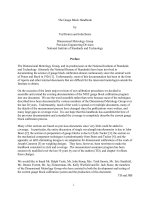
Figure 6.11 shows a graphical output of the NIST multicolor interferometry program using a
cadmium light source. The program calculates the actual wavelengths for each color using the
environmental factors (air temperature, pressure and humidity). Then, using the observed fringe
fraction, shows the possible lengths of the gauge block which are near the nominal length for each
color. Note that the possible lengths are shown as small bars, with their width corresponding to the
uncertainty in the fringe fraction.

114

Figure 6.12. Graphical output of the NIST multicolor interferometry program.
The length at which all the colors match within 0.030 µm is assumed to be the
true gauge block length. The match is at -0.09 µm in this example.


The length where all of the fringes overlap is the actual length of the block. If all the fringes do not
overlap in the set with the best fit, the inconsistency is taken as evidence of an operator error and the
block is re-measured. The computer is also programmed to examine the data and decide if there is a
length reasonably close to the nominal length for which the different wavelengths agree to a given
tolerance. As a rule of thumb, all of the wavelengths should agree to better than 0.030 µm to be
acceptable.

Analytic methods for analyzing multicolor interferometry have also been developed [49]. Our
implementations of these types of methods have not performed well. The problem is probably that
the span of wavelengths available, being restricted to the visible, is not wide enough and the fringe
fraction measurement not precise enough for the algorithms to work unambiguously.


6.9 Use of the Linescale Interferometer for End Standard Calibration

There are a number of methods to calibrate a gauge block of completely unknown length. The
multiple wavelength interferometry of the previous section is used extensively, but has the limitation
that most atomic sources have very limited coherence lengths, usually under 25 mm. The method
can be used by measuring a set of blocks against each other in a sequence to generate the longest
length. For example, for a 10 inch block, a 1 inch block can be measured absolutely followed by

differential measurements of a 2 inch block with the 1 inch block, a 3 inch block with the 2, a 4 inch
block with the 3, a 5 inch block with the 4, and the 10 inch block with the 2, 3 and 5 inch blocks
0 1 2 3 .1 .2 .3
Micrometers from Nominal
4 .4
Laser
Cd Red
Cd Green
Cd Blue
Cd Violet

115
wrung together. Needless to say this method is tedious and involves the uncertainties of a large
number of measurements.

Another, simpler, method is to convert a long end standard into a line standard and measure it with
an instrument designed to measure or compare line scales (for example, meter bars) [51]. The NIST
linescale interferometer, shown schematically below, is generally used to check our master blocks
over 250 mm long to assure that the length is known within the 1/2 fringe needed for single
wavelength interferometry.

The linescale interferometer consists of a 2 m long waybed which moves a scale up to a meter in
length, under a microscope. An automated photoelectric microscope, sends a servo signal to the
machine controller which moves the scale so that the graduation is at a null position on the
microscope field of view. A laser interferometer measures the distances between the marks on the
scale via a corner cube attached to one end of the scale support. This system is described in detail
elsewhere [52,53].

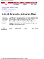
To measure an end standard, two small gauge blocks that have linescale graduations on one side, are
wrung to the ends of the end standard, as shown in figure 6.13. This "scale" is then measured on the

linescale interferometer. The gauge blocks are then removed from the end standard and wrung
together, forming a short scale. This "scale" is also measured on the interferometer. The difference
in length between the two measurements is the physical distance between the end faces of the end
standard plus one wringing film. This distance is the defined length of the end standard.



















Figure 6.13. Two small gauge blocks with linescale graduations on
one side are wrung to the ends of the end standard, allowing the end
standard to be measured as a linescale.


116
The only significant problem with this method is that it is not a platen to gauge point measurement

like a normal interferometric measurement. If the end standard faces are not flat and parallel the
measurement will not give the exact same length, although knowledge of the parallelism and flatness
will allow corrections to be made. Since the method is only used to determine the length within 1/2
fringe of the true length this correction is seldom needed.


117
7. References

[1] C.G. Peters and H.S. Boyd, "Interference methods for standardizing and testing precision
gauge blocks," Scientific Papers of the Bureau of Standards, Vol. 17, p.691 (1922).

[2] Beers, J.S. "A Gauge Block Measurement Process Using Single Wavelength Interferometry,"
NBS Monograph 152, 1975.

[3] Tucker, C.D. "Preparations for Gauge Block Comparison Measurements," NBSIR 74-523.

[4] Beers, J.S. and C.D. Tucker. "Intercomparison Procedures for Gauge Blocks Using
Electromechanical Comparators," NBSIR 76-979.

[5] Cameron, J.M. and G.E Hailes. "Designs for the Calibration of Small Groups of Standards in
the Presence of Drift," NBS Technical Note 844, 1974.

[6] Klein, Herbert A., The Science of Measurement
, Dover Publications, 1988.

[7] Galyer, J.F.W. and C.R. Shotbolt, Metrology for Engineers, Cassel & Company, Ltd.,
London, 1964.

[8] "Documents Concerning the New Definition of the Meter," Metrologia, Vol. 19, 1984.

[9] "Use of the International Inch for Reporting Lengths of Gauge Blocks," National Bureau of
Standards (U.S.) Letter Circular LC-1033, May, 1959.

[10] T.K.W. Althin, C.E. Johansson, 1864-1943, Stockolm, 1948.

[11] Cochrane, Rexmond C., AMeasures for Progress," National Bureau of Standards (U.S.),
1966.

[12] Federal Specification: Gauge Blocks and Accessories (Inch and Metric)
, Federal
Specification GGG-G-15C, March 20, 1975.

[13] Precision Gauge Blocks for Length Measurement (Through 20 in. and 500 mm),
ANSI/ASME B89.1.9M-1984, The American Society of Mechanical Engineers, 1984.

[14] International Standard 3650, Gauge Blocks, First Edition, 1978-07-15, 1978

[15] DIN 861, part 1, Gauge Blocks: Concepts, requirements, testing
, January 1983.

[16] M.R. Meyerson, T.R. Young and W.R. Ney, "Gauge Blocks of Superior Stability: Initial
Developments in Materials and Measurement," J. of Research of the National Bureau of
Standards, Vol. 64C, No. 3, 1960.


118
[17] Meyerson, M.R., P.M. Giles and P.F. Newfeld, "Dimensional Stability of Gauge Block
Materials," J. of Materials, Vol. 3, No. 4, 1968.

[18] Birch, K.P., "An automatic absolute interferometric dilatometer," J. Phys. E: Sci. Instrum,
Vol. 20, 1987.

[19] J.W. Berthold, S.F. Jacobs and M.A. Norton, "Dimensional Stability of Fused Silica, Invar,
and Several Ultra-low Thermal Expansion Materials," Metrologia, Vol. 13, pp. 9-16 (1977).

[20] C.W. Marshall and R.E. Maringer, Dimensional Instability, An Introduction
, Pergamon
Press, New York (1977).

[21] Hertz, H., "On the contact of elastic solids," English translation in Miscellaneous Papers,
Macmillan, N.Y., 1896.

[22] Poole, S.P., "New method of measuring the diameters of balls to a high precision,"
Machinery, Vol 101, 1961.

[23] Norden, Nelson B., "On the Compression of a Cylinder in Contact with a Plane Surface,"
NBSIR 73-243, 1973.

[24] Puttock, M.J. and E.G. Thwaite, "Elastic Compression of Spheres and Cylinders at Point and
Line Contact," National Standards Laboratory Technical Paper No. 25, CSIRO, 1969.

[25] Beers, John, and James E. Taylor, "Contact Deformation in Gauge Block Comparisons,"
NBS Technical Note 962, 1978

[26] Beyer-Helms, F., H. Darnedde, and G. Exner. "Langenstabilitat bei Raumtemperatur von
Proben er Glaskeramik 'Zerodur'," Metrologia Vol. 21, p49-57 (1985).

[27] Berthold, J.W. III, S.F. Jacobs, and M.A. Norton. "Dimensional Stability of Fused Silica,
Invar, and Several Ultra-low Thermal Expansion Materials," Metrologia, Vol. 13, p9-16

(1977).

[28] Justice, B., "Precision Measurements of the Dimensional Stability of Four Mirror Materials,"
Journal of Research of the National Bureau of Standards - A: Physics and Chemistry, Vol.
79A, No. 4, 1975.

[29] Bruce, C.F., Duffy, R.M., Applied Optics Vol.9, p743-747 (1970).

[30] Average of 1,2,3 and 4 inch steel master gauge blocks at N.I.S.T.

[31] Doiron, T., Stoup, J., Chaconas, G. and Snoots, P. "stability paper, SPIE".

[32] Eisenhart, Churchill, "Realistic Evaluation of the Precision and Accuracy of Instrument

119
Calibration Systems," Journal of Research of the National Bureau of Standards, Vol. 67C,
No. 2, pp. 161-187, 1963.

[33] Croarkin, Carroll, "Measurement Assurance Programs, Part II: Development and
Implementation," NBS Special Publication 676-II, 1984.

[34] ISO, "Guide to the Expression of Uncertainty in Measurement," October 1993.

[35] Taylor, Barry N. and Chris E. Kuyatt, "Guidelines for Evaluating and Expressing the
Uncertainty of NIST Measurement Results," NIST Technical Note 1297, 1994 Edition,
September 1994.

[36] Tan, A. and J.R. Miller, "Trend studies of standard and regular gauge block sets," Review of
Scientific Instruments, V.62, No. 1, pp.233-237, 1991.

[37] C.F. Bruce, "The Effects of Collimation and Oblique Incidence in Length Interferometers. I,"
Australian Journal of Physics, Vol. 8, pp. 224-240 (1955).

[38] C.F. Bruce, "Obliquity Correction Curves for Use in Length Interferometry," J. of the
Optical Society of America, Vol. 45, No. 12, pp. 1084-1085 (1955).

[39] B.S. Thornton, "The Effects of Collimation and Oblique Incidence in Length
Interferometry," Australian Journal of Physics, Vol. 8, pp. 241-247 (1955).

[40] L. Miller, Engineering Dimensional Metrology
, Edward Arnold, Ltd., London (1962).

[41] Schweitzer, W.G., et.al., "Description, Performance and Wavelengths of Iodine Stabilized
Lasers," Applied Optics, Vol 12, 1973.

[42] Chartier, J.M., et. al., "Intercomparison of Northern European
127
I
2
- Stabilized He-Ne
Lasers at
λ = 633 nm," Metrologia, Vol 29, 1992.

[43] Balhorn, R., H. Kunzmann and F. Lebowsky, AFrequency Stabilization of Internal-Mirror
Helium-Neon Lasers,@ Applied Optics, Vol 11/4, April 1972.

[44] Mangum, B.W. and G.T. Furukawa, "Guidelines for Realizing the International Temperature
Scale of 1990 (ITS-90)," NIST Technical Note 1265, National Institute of Standards and
Tecnology, 1990.

[45] Edlen, B., "The Refractive Index of Air," Metrologia, Vol. 2, No. 2, 1966.

[46] Schellekens, P., G. WIlkening, F. Reinboth, M.J. Downs, K.P. Birch, and J. Spronck,
"Measurements of the Refractive Index of Air Using Interference Refractometers,"
Metrologia, Vol. 22, 1986.


120
[47] Birch, K.P. and Downs, M.J., "The results of a comparison between calculated and measured
values of the refractive index of air," J. Phys. E: Sci. Instrum., Vol. 21, pp. 694-695, 1988.

[48] Birch, K.P. and M.J. Downs, "Correction to the Updated Edlén Equation for the Refractive
Index of Air," Metrologia, Vol. 31, 1994.

[49] C.R. Tilford, "Analytical Procedure for determining lengths from fractional fringes," Applied
Optics, Vol. 16, No. 7, pp. 1857-1860 (1977).

[50] F.H. Rolt, Gauges and Fine Measurements
, Macmillan and Co., Limited, 1929.

[51] Beers, J.S. and Kang B. Lee, "Interferometric measurement of length scales at the National
Bureau of Standards," Precision Engineering, Vol. 4, No. 4, 1982.

[52] Beers, J.S., "Length Scale Measurement Procedures at the National Bureau of Standards,"
NBSIR 87-3625, 1987.

[53] Beers, John S. and William B. Penzes, "NIST Length Scale Interferometer Measurement
Assurance," NISTIR 4998, 1992.

121
APPENDIX A. Drift Eliminating Designs for Non-simultaneous Comparison
Calibrations


Introduction

The sources of variation in measurements are numerous. Some of the sources are truly random
noise, 1/f noise in electronic circuits for example. Usually the "noise" of a measurement is actually
due to uncontrolled systematic effects such as instability of the mechanical setup or variations in the
conditions or procedures of the test. Many of these variations are random in the sense that they are
describable by a normal distribution. Like true noise in the measurement system, the effects can be
reduced by making additional measurements.

Another source of serious problems, which is not random, is drift in the instrument readings. This
effect cannot be minimized by additional measurement because it is not generally pseudo-random,
but a nearly monotonic shift in the readings. In dimensional metrology the most import cause of
drift is thermal changes in the equipment during the test. In this paper we will demonstrate
techniques to address this problem of instrument drift.

A simple example of the techniques for eliminating the effects of drift by looking at two different
ways of comparing 2 gauge blocks, one standard (A) and one unknown (B).

Scheme 1: A B A B

Scheme 2: A B B A

Now let us suppose we make the measurements regularly spaced in time, 1 time unit apart, and there

is an instrumental drift of ∆. The actual readings (y
i
) from scheme 1 are:

y
1
= A (A.1a)
y
2
= B + ∆ (A.1b)
y
3
= A + 2∆ (A.1c)
y
4
= B + 3∆ (A.1d)


Solving for B in terms of A we get:


(A.2)


which depends on the drift rate ∆.

Now look at scheme 2. Under the identical conditions the readings are:

-Y4)-Y2-Y3+(Y1
2

1
-A=B ∆

122
y
1
= A (A.3a)
y
2
= B + ∆ (A.3b)
y
3
= B + 2∆ (A.3c)
y
4
= A + 3∆ (A.3d)

Here we see that if we add the second and third readings and subtract the first and fourth readings we
find that the ∆ drops out:


(A.4)


Thus if the drift rate is constant - a fair approximation for most measurements if the time is properly
restricted - the analysis both eliminates the drift and supplies a numerical approximation of the drift
rate.

The calibration of a small number of "unknown" objects relative to one or two reference standards
involves determining differences among the group of objects. Instrumental drift, due most often to

temperature effects, can bias both the values assigned to the objects and the estimate of the effect of
random errors. This appendix presents schedules for sequential measurements of differences that
eliminate the bias from these sources and at the same time gives estimates of the magnitude of these
extraneous components.

Previous works have [A1,A2] discussed schemes which eliminate the effects of drift for
simultaneous comparisons of objects. For these types of measurements the difference between two
objects is determined at one instant of time. Examples of these types of measurements are
comparisons of masses with a double pan balance, comparison of standard voltage cells, and
thermometers which are all placed in the same thermalizing environment. Many comparisons,
especially those in dimensional metrology, cannot be done simultaneously. For example, using a
gauge block comparator, the standard, control (check standard) and test blocks are moved one at a
time under the measurement stylus. For these comparisons each measurement is made at a different
time. Schemes which assume simultaneous measurements will, in fact, eliminate the drift from the
analysis of the test objects but will produce a measurement variance which is drift dependent and an
erroneous value for the drift, ∆.

In these calibration designs only differences between items are measured so that unless one or more
of them are standards for which values are known, one cannot assign values for the remaining
"unknown" items. Algebraically, one has a system of equations that is not of full rank and needs the
value for one item or the sum of several items as the restraint to lead to a unique solution. The least
squares method used in solving these equations has been presented [A3] and refined [A4] in the
literature and will not be repeated in detail here. The analyses presented of particular measurement
designs presented later in this paper conform to the method and notation presented in detail by
Hughes [A3].

The schemes used as examples in this paper are those currently used at NIST for gauge block
Y3)-Y2-Y4+(Y1
2
1

-A=B

123
comparisons. In our calibrations a control (check standard) is always used to generate data for our
measurement assurance plan [A5]. It is not necessary, however, to use a control in every
measurement and the schemes presented can be used with any of the objects as the standard and the
rest as unknowns. A number of schemes of various numbers of unknowns and measurements is
presented in the appendix.


Calibration Designs

The term calibration design has been applied to experiments where only differences between
nominally equal objects or groups of objects can be measured. Perhaps the simplest such
experiment consists in measuring the differences between the two objects of the n(n-1) distinct
pairings that can be formed from n objects. If the order is unimportant, X compared to Y is the
negative of Y compared to X, there are only n(n-1)/2 distinct pairings. Of course only 1
measurement per unknown is needed to determine the unknown, but many more measurements are
generally taken for statistical reasons. Ordinarily the order in which these measurements are made is
of no consequence. However, when the response of the comparator is time dependent, attention to
the order is important if one wished to minimize the effect of these changes.

When this effect can be adequately represented by a linear drift, it is possible to balance out the
effect by proper ordering of the observations. The drift can be represented by the series, . . . -3 , -2 ,
-1 , 0, 1, 2 , 3 , . . . if there are an odd number of comparisons and by -5/2 , -3/2 , -1/2 , 1/2 , 3/2 ,
5/2 , if there are an even number of comparisons.

As and example let us take n=3. If we make all possible n(n-1)=6 comparisons we get a scheme like
that below, denoting the three objects by A, B, C.

Observation
Measurement

m
1
A - 11/2 ∆
m
2
B - 9/2 ∆
m
3
C - 7/2 ∆
m
4
A - 5/2 ∆
m
5
B - 3/ 2 ∆
m
6
C - 1/2 ∆ (A.5)
m
7
A + 1/2 ∆
m
8
C + 3/2 ∆
m
9
B + 5/2 ∆

m
10
A + 7/2 ∆
m
11
C + 9/2 ∆
m
12
B + 11/2 ∆


If we analyze these measurements by pairs, in analogy to the weighing designs of Cameron we see
that:

124


A B C ∆
y
1
= m
1
- m
2
= A - B - ∆ +1 - 1 -1
y
2
= m
3
- m

4
= C - A - ∆ - 1 +1 -1
y
3
= m
5
- m
6
= B - C - ∆ +1 - 1 -1 (A.6)
y
4
= m
7
- m
8
= A - C - ∆ +1 - 1 -1
y
5
= m
9
- m
10
= B - A - ∆ - 1 +1 -1
y
6
= m
11
- m
12
= C - B - ∆ - 1 +1 -1

The notation used here, the plus and minus signs, indicate the items entering into the difference
measurement. Thus, y
2
is a measurement of the difference between object C and object A.

Note the difference between the above table and that of simultaneous comparisons in reference 2 is
that the drift column is constant. It is simple to see by inspection that the drift is balanced out since
each object has two (+) and two (-) measurements and the drift column is constant. By extension,
the effects of linear drift is eliminated in all complete block measurement schemes (those for which
all objects are measured in all possible n(n-1) combinations).

Although all schemes in which each object has equal numbers of (+) and (-) measurements is drift
eliminating, there are practical criteria which must be met for the scheme to work. First, the actual
drift must be linear. For dimensional measurements the instrument drift is usually due to changes in
temperature. The usefulness of drift eliminating designs depends on the stability of the thermal
environment and the accuracy required in the calibration. In the NIST gauge block lab the
environment is stable enough that the drift is linear at the 3 nm (0.1 µin) level over periods of 5 to
10 minutes. Our comparison plans are chosen so that the measurements can be made in this period.
Secondly, each measurement must be made in about the same amount of time so that the
measurements are made at fairly regular intervals. In a completely automated system this is simple,
but with human operators there is a natural tendency to make measurements simpler and quicker is
the opportunity presents itself. For example, if the scheme has a single block measured two or more
times in succession it is tempting to measure the object without removing it from the apparatus,
placing it in its normal resting position, and returning it to the apparatus for the next measurement.

Finally, the measurements of each block are spread as evenly as possible across the design. Suppose
in the scheme above where each block is measured 4 times block, A is measured as the first
measurement of y

1
, y
2
, y
3
, and y
4
. There is a tendency to leave block A near the measuring point
rather than its normal resting position because it is used so often in the first part of the scheme. This
allows block A to have a different thermal handling than the other blocks which can result in a
thermal drift which is not the same as the other blocks.

Restraints

Since all of the measurements made in a calibration are relative comparisons, at least one value must
be known to solve the system of equations. In the design of the last section, for example, if one has

125
a single standard and two unknowns, the standard can be assigned to any one of the letters. (The
same would be true of three standards and one unknown.) If there are two standards and one
unknown, the choice of which pair of letters to assign for the standards is important in terms of
minimizing the uncertainty in the unknown.

For full block designs (all possible comparisons are made) there is no difference which label is used
for the standards or unknowns. For incomplete block designs the uncertainty of the results can
depend on which letter the standard and unknowns are assigned. In these cases the customer blocks
are assigned to minimize their variance and allow the larger variance for the measurement of the
extra master (control).

This asymmetry occurs because every possible comparison between the four items has not been

measured. For 4 objects there are 12 possible intercomparisons. If an 8 measurement scheme is
used all three unknowns cannot be compared directly to the standard the same number of times. For
example, two unknowns can be compared directly with the standard twice, but the other unknown
will have no direct comparisons. This indirect comparison to the standard results in a slightly larger
variance for the block compared indirectly. Complete block plans, which compare each block to
every other block equal number of times, have no such asymmetry, and thus remove any restriction
on the measurement position of the control.


Example: 4 block, 12 comparison, Single Restraint Design for NIST Gauge Block Calibration

The gauge block comparison scheme put into operation in 1989 consists of two standards blocks,
denoted S and C, and two customer blocks to be calibrated, denoted X and Y. In order to decrease
the random error of the comparison process a new scheme was devised consisting of all 12 possible
comparisons between the four blocks. Because of continuing problems making penetration
corrections, the scheme was designed to use either the S or C block as the restraint and the difference
(S-C) as the control parameter. The S blocks are all steel, and are used as the restraint for all steel
customer blocks. The C blocks are chrome carbide, and are used as the restraint for chrome and
tungsten carbide blocks. The difference (S-C) is independent of the choice of restraint.

We chose a complete block scheme that assures that the design is drift eliminating, and the blocks
can be assigned to the letters of the design arbitrarily. We chose (S-C) as the first comparison.
Since there are a large number of ways to arrange the 12 measurements for a complete block design,
we added two restrictions as a guide to choose a "best" design.

1. Since the blocks are measured one at a time, it was decided to avoid schemes which measured
the same block two or more times consecutively. In the scheme presented earlier blocks D, A
and C are all measured twice consecutively. There is a great temptation to not remove and
replace the blocks under these conditions, and the scheme assumes that each measurement is
made with the same motion and are evenly spaced in time. This repetition threatens both these

assumptions.

2. We decided that schemes in which the six measurements of each block were spread out as

126
evenly as possible in time would be less likely to be affected by small non-linearities in the drift.
For example, some schemes had one block finished its 6 measurements by the 8th comparison,
leaving the final 1/3 of the comparisons with no sampling of that block.


The new scheme is as follows: S C X Y ∆


XY
SX
CX
YS
YC
XS
XY
XC
SC
YX
SY
CS
Y
Y
Y
Y
Y

Y
Y
Y
Y
Y
Y
Y
Y
−
−
−
−
−
−
−
−
−
−
−
−
==
12
11
10
9
8
7
6
5
4

3
2
1

11100
10101
10110
11001
11010
10101
11010
10110
10011
11100
11001
10011
−−
−−
−−
−−
−−
−−
−−
−−
−−
−−
−−
−
−
=X

(A.7)


When the S block is the restraint (S – L) the matrix equation to solve is:



L
YX
a
aXX
A
t
t
t
•=
−1
0
(A.8)

| a
t
| = [ 1 0 0 0 ] (A.9)


000001
0120000
006222
002622
002262

102226
0
−−−
−−−
−−−
−−−
==
t
t
ij
a
aXX
C (A.10)