compilers principles techniques and tools phần 7 pptx
Bạn đang xem bản rút gọn của tài liệu. Xem và tải ngay bản đầy đủ của tài liệu tại đây (5.01 MB, 104 trang )
602
CHAPTER
9.
MACHINE-INDEPENDENT OPTIMIZATIONS
Detecting Possible Uses Before Definition
Here is how we use a solution to the reaching-definitions problem to detect
uses before definition. The trick is to introduce a dummy definition for
each variable
x
in the entry to the flow graph. If the dummy definition
of
x
reaches a point
p
where
x
might be used, then there might be an
opportunity to use
x
before definition. Note that we can never be abso-
lutely certain that the program has a bug, since there may be some reason,
possibly involving a complex logical argument, why the path along which
p
is reached without a real definition of
x
can never be taken.
know whether a statement
s
is assigning a value to
x,
we must assume that
it
may
assign to it; that is, variable
x
after statement
s
may have either its
original value before
s
or the new value created by
s.
For the sake of simplicity,
the rest of the chapter assumes that we are dealing only with variables that
have no aliases. This class of variables includes all local scalar variables in most
languages; in the case of C and
C++, local variables whose addresses have been
computed at some point are excluded.
Example
9.9
:
Shown in Fig.
9.13
is a flow graph with seven definitions. Let us
focus on the definitions reaching block
B2. All the definitions in block B1 reach
the beginning of block
B2. The definition ds:
j
=
j-1
in block B2 also reaches
the beginning of block
B2, because no other definitions of
j
can be found in the
loop leading back to
B2. This definition, however, kills the definition d2:
j
=
n,
preventing it from reaching B3 or B4. The statement d4:
i
=
i+l
in B2 does
not reach the beginning of
B2 though, because the variable
i
is always redefined
by
d7:
i
=
u3.
Finally, the definition ds
:
a
=
u2
also reaches the beginning of
block
B2.
By defining reaching definitions as we have, we sometimes allow inaccuracies.
However, they are all in the
"safe," or "conservative," direction. For example,
notice our assumption that all edges of a flow graph can be traversed. This
assumption may not be true in practice. For example, for no values of
a
and
b
can the flow of control actually reach
statement
2
in the following program
fragment:
if
(a
==
b)
statement
1;
else
if
(a
==
b)
statement
2;
To decide in general whether each path in a flow graph can be taken is
an undecidable problem. Thus, we simply assume that every path in the flow
graph can be followed in some execution of the program. In most applications
of reaching definitions, it is conservative to assume that a definition can reach a
point even if it might not. Thus, we may allow paths that are never be traversed
in any execution of the program, and we may allow definitions to pass through
ambiguous definitions of the same variable safely.
Simpo PDF Merge and Split Unregistered Version -
9.2.
INTRODUCTION TO DATA-FLO
W
ANALYSIS
603
Conservatism in Data-Flow Analysis
Since all data-flow schemas compute approximations to the ground truth
(as defined by all possible execution paths of the program), we are obliged
to assure that any errors are in the "safe" direction. A policy decision is
safe (or conservative) if it never allows us to change what the program
computes. Safe policies may, unfortunately, cause us to miss some code
improvements that would retain the meaning of the program, but in essen-
tially all code optimizations there is no safe policy that misses nothing. It
would generally be unacceptable to use an unsafe policy
-
one that sped'
up the code at the expense of changing what the program computes.
Thus, when designing a data-flow schema, we must be conscious of
how the information will be used, and make sure that any approximations
we make are in the "conservative" or "safe" direction. Each schema and
application must be considered independently. For instance, if we use
reaching definitions for constant folding, it is safe to think a definition
reaches when it doesn't (we might think x is not a constant, when in fact
it is and could have been folded), but not safe to think a definition doesn't
reach when it does (we might replace x by a constant, when the program
would at times have a value for
x
other than that constant).
Transfer Equations for Reaching Definitions
We shall now set up the constraints for the reaching definitions problem. We
start by examining the details of a single statement. Consider a definition
Here, and frequently in what follows,
+
is used as a generic binary operator.
This statement "generates" a definition
d
of variable u and "kills" all the
other definitions in the program that define variable u, while leaving the re-
maining incoming definitions unaffected. The transfer function of definition
d
thus can be expressed as
where
gend
=
{d},
the set of definitions generated by the statement, and killd
is the set of all other definitions of u in the program.
As discussed in Section 9.2.2, the transfer function of a basic block can be
found by composing the transfer functions of the statements contained therein.
The composition of functions of the form
(9.1), which we shall refer to as "gen-
kill form," is also of that form, as we can see as follows. Suppose there are two
functions
f~(x)
=
genl
U
(x
-
M111) and f2(x)
=
genz
U
(x
-
killz). Then
Simpo PDF Merge and Split Unregistered Version -
604
CHAPTER
9.
MACHINE-INDEPENDENT OPTIMIZATIONS
ENTRY
'
gen
=
{
d6
1
B3
kill
={4}
B3
senB4
={
d,
1
kill
=
{
dl, d4
}
B4
Figure
9.13:
Flow graph for illustrating reaching definitions
This rule extends to a block consisting of any number of statements. Suppose
block
B
has
n
statements, with transfer functions
fi(x)
=
geni
U
(x
-
killi)
for
i
=
1,2,
.
.
.
,
n.
Then the transfer function for block
B
may be written as:
where
killB
=
killl
U
kill2
U
.
-
.
U
kill,
and
gen~
=
gen,
U
(gen,-1
-
kill,)
U
(gennV2
-
-
kill,)
U
-
-
.
U
(genl
-
killz
-
kills
-
.
-
.
-
kill,)
Simpo PDF Merge and Split Unregistered Version -
9.2.
INTRODUCTION TO DATA-FLO
W
ANALYSIS
Thus, like a statement, a basic block also generates a set of definitions and
kills a set of definitions. The
gen
set contains all the definitions inside the block
that are "visible" immediately after the block
-
we refer to them as
downwards
exposed.
A
definition is downwards exposed in a basic block only if it is not
"killed" by a subsequent definition to the same variable inside the same basic
block.
A
basic block's
kill
set is simply the union of all the definitions killed by
the individual statements. Notice that
a
definition may appear in both the
gen
and
kill
set of a basic block. If so, the fact that it is in
gen
takes precedence,
because in
gen-kill
form, the
kill
set is applied before the
gen
set.
Example
9.10
:
The
gen
set for the basic block
is
Id2) since
dl
is not downwards exposed. The
kill
set contains both dl and
d2, since
dl
kills d2 and vice versa. Nonetheless, since the subtraction of the
kill
set precedes the union operation with the
gen
set, the result of the transfer
function for this block always includes definition
dz.
Control-Flow Equations
Next, we consider the set of constraints derived from the control flow between
basic blocks. Since a definition reaches a program point as long as there exists
at least one path along which the definition reaches,
OUT[P]
C
IN[B] whenever
there is a control-flow edge from
P
to
B.
However, since a definition cannot
reach a point unless there is a path along which it reaches,
IN[B] needs to be no
larger than the union of the reaching definitions of all the predecessor blocks.
That is, it is safe to assume
UP
a
predecessor of
B
OUT[P]
We refer to union as the
meet operator
for reaching definitions. In any data-
flow schema, the meet operator is the one we use to create a summary of the
contributions from different paths at the confluence of those paths.
Iterative Algorithm for Reaching Definitions
We assume that every control-flow graph has two empty basic blocks, an
ENTRY
node, which represents the starting point of the graph, and an
EXIT
node to
which all exits out of the graph go. Since no definitions reach the beginning
of the graph, the transfer function for the
ENTRY
block is a simple constant
function that returns
0
as an answer. That is,
OUT[ENTRY]
=
0.
The reaching definitions problem is defined by the following equations:
Simpo PDF Merge and Split Unregistered Version -
606
CHAPTER
9.
MACHINE-INDEPENDENT OPTIMIZATIONS
and for all basic blocks B other than
ENTRY,
OUT[B]
=
geng
U
(IN[B]
-
killB)
UP
a predecessor of
B
OUT[P].
These equations can be solved using the following algorithm. The result of
the algorithm is the least
fixedpoint of the equations, i.e., the solution whose
assigned values to the
IN'S
and
OUT'S
is contained in the corresponding values
for any other solution to the equations. The result of the algorithm below is
acceptable, since any definition in one of the sets
IN
or OUT surely must reach
the point described.
It is a desirable solution, since it does not include any
definitions that we can be sure do not reach.
Algorithm
9.11
:
Reaching definitions.
INPUT:
A
flow graph for which killB and gen~ have been computed for each
block
B.
OUTPUT:
IN[B] and OUT[B], the set of definitions reaching the entry and exit
of each block
B
of the flow graph.
METHOD:
We use an iterative approach, in which we start with the "estimate"
OUT[B]
=
0
for all B and converge to the desired values of
IN
and OUT. As
we must iterate until the
IN'S
(and hence the OUT'S) converge, we could use a
boolean variable change to record, on each pass through the blocks, whether
any
OUT
has changed. However, in this and in similar algorithms described
later, we assume that the exact mechanism for keeping track of changes is
understood, and we elide those details.
The algorithm is sketched in Fig. 9.14. The first two lines initialize certain
data-flow
value^.^
Line
(3)
starts the loop in which we iterate until convergence,
and the inner loop of lines
(4)
through
(6)
applies the data-flow equations to
every block other than the entry.
Intuitively, Algorithm 9.11 propagates definitions as far as they will go with-
out being killed, thus simulating all possible executions of the program. Algo-
rithm 9.11 will eventually halt, because for every B,
OUT[B] never shrinks; once
a definition is added, it stays there forever. (See Exercise 9.2.6.) Since the set of
all definitions is finite, eventually there must be a pass of the while-loop during
which nothing is added to any
OUT,
and the algorithm then terminates. We
are safe terminating then because if the
OUT'S
have not changed, the
IN'S
will
4~he observant reader will notice that we could easily combine lines (1) and
(2).
However,
in similar data-flow algorithms, it may be necessary to initialize the entry or exit node dif-
ferently from the way we initialize the other nodes. Thus, we follow
a
pattern
in
all iterative
algorithms of applying a "boundary condition" like line (1) separately from the initialization
of line
(2).
Simpo PDF Merge and Split Unregistered Version -
9.2.
INTRODUCTION TO DATA-FLOW ANALYSIS
1) OUT[ENTRY]
=
0;
2)
for
(each basic block B other than ENTRY) OUT[B]
=
0;
3)
while
(changes to any OUT occur)
4)
for
(each basic block
B
other than ENTRY)
{
5)
=
UP
a
predecessor of
B
OuTIP1;
6)
OUT[B]
=
geng
U
(IN[B]
-
killB);
}
Figure 9.14: Iterative algorithm to compute reaching definitions
not change on the next pass. And, if the
IN'S
do not change, the OUT'S cannot,
so on all subsequent passes there can be no changes.
The number of nodes in the flow graph is an upper bound on the number of
times around the while-loop. The reason is that if a definition reaches a point,
it can do so along a cycle-free path, and the number of nodes in a flow graph is
an upper bound on the number of nodes in a cycle-free path. Each time around
the while-loop, each definition progresses by at least one node along the path
in question, and it often progresses by more than one node, depending on the
order in which the nodes are visited.
In fact, if we properly order the blocks in the for-loop of line
(5), there
is empirical evidence that the average number of iterations of the while-loop
is under 5 (see Section 9.6.7). Since sets of definitions can be represented
by bit vectors, and the operations on these sets can be implemented by logical
operations on the bit vectors, Algorithm 9.11 is surprisingly efficient in practice.
Example
9.12
:
We shall represent the seven definitions dl, d2,
. . .
,
d7
in the
flow graph of Fig. 9.13 by bit vectors, where bit
i
from the left represents
definition
di. The union of sets is computed by taking the logical
OR
of the
corresponding bit vectors.
The difference of two sets
S
-
T
is computed by
complementing the bit vector of
T,
and then taking the logical
AND
of that
complement, with the bit vector for
S.
Shown in the table of Fig. 9.15 are the values taken on by the
IN
and
OUT
sets in Algorithm 9.11. The initial values, indicated by a superscript 0, as
in
OUT[B]O, are assigned, by the loop of line
(2)
of Fig. 9.14. They are each
the empty set, represented by bit vector 000 0000. The values of subsequent
passes of the algorithm are also indicated by superscripts, and labeled
1N[BI1
and OUT[B]' for the first pass and 1N[BI2 and 0uT[BI2 for the second.
Suppose the for-loop of lines (4) through
(6)
is executed with B taking on
the values
in that order. With
B
=
B1, since
OUT[ENTRY]
=
0,
IN[B~]' is the empty set,
and
OUT[B~]~ is
geng,.
This value differs from the previous value OUT[B~]~, so
Simpo PDF Merge and Split Unregistered Version -
608
CHAPTER
9.
MACHINE-INDEPENDENT OPTIMIZATIONS
Figure
9.15:
Computation of
IN
and
OUT
Block B
B1
B2
BS
B4
EXIT
we now know there is a change on the first round (and will proceed to a second
round).
Then we consider B
=
B2 and compute
This computation is summarized in Fig.
9.15.
For instance, at the end of the
first pass,
0UT[B2I1
=
001 1100,
reflecting the fact that
d4
and
d5
are generated
in
B2, while
d3
reaches the beginning of B2 and is not killed in B2.
Notice that after the second round, 0UT[B2] has changed to reflect the fact
that
d6
also reaches the beginning of B2 and is not killed by B2. We did not
learn that fact on the first pass, because the path from
ds
to the end of B2,
which is
B3
-+
B4
-+
B2, is not traversed in that order by a single pass. That is,
by the time we learn that
d6
reaches the end of B4, we have already computed
IN[B~] and 0uT[B2] on the first pass.
There are no changes in any of the
OUT
sets after the second pass. Thus,
after a third pass, the algorithm terminates, with the
IN'S
and
OUT'S
as in the
final two columns of Fig.
9.15.
OUT[B]O
000 0000
000 0000
000 0000
000 0000
000 0000
9.2.5
Live-Variable Analysis
Some code-improving transformations depend on information computed in the
direction opposite to the flow of control in a program; we shall examine one
such example now. In
live-variable analysis
we wish to know for variable
x
and
point
p
whether the value of
x
at
p
could be used along some path in the flow
graph starting at
p.
If so, we say
x
is
live
at
p;
otherwise,
x
is
dead
at
p.
An important use for live-variable information is register allocation for basic
blocks. Aspects of this issue were introduced in Sections
8.6
and
8.8.
After a
value is computed in a register, and presumably used within a block, it is not
1N[BI1
000 0000
111
0000
001 1100
001 1110
001 0111
OUT[B]~
111
0000
001
1100
000 1110
001 0111
001 0111
1N[BI2
000 0000
111 0111
001 1110
001 1110
001 0111
OUT[B]~
111
0000
001 1110
000 1110
001 0111
001 0111
Simpo PDF Merge and Split Unregistered Version -
9.2.
INTRODUCTION TO DATA-FLO
W
ANALYSIS 609
necessary to store that value if it is dead at the end of the block. Also, if all
registers are full and we need another register, we should favor using a register
with a dead value, since that value does not have to be stored.
Here, we define the data-flow equations directly in terms of
IN[B] and
OUT[B], which represent the set of variables live at the points immediately
before and after block B, respectively.
These equations can also be derived
by first defining the transfer functions of individual statements and composing
them to create the transfer function of a basic block. Define
1.
defB
as the set of variables
defined
(i.e., definitely assigned values) in B
prior to any use of that variable in B, and
2.
useg
as the set of variables whose values may be used in B prior to any
definition of the variable.
Example
9.13
:
For instance, block B2 in Fig. 9.13 definitely uses i. It also
uses
j
before any redefinition of
j,
unless it is possible that i and
j
are aliases
of one another. Assuming there are no aliases among the variables in Fig. 9.13,
then
use^,
=
{i,
j).
Also, B2 clearly defines i and
j.
Assuming there are no
aliases,
defg,
=
{i,
j),
as well.
As a consequence of the definitions, any variable in
use^
must be considered
live on entrance to block B, while definitions of variables in
defB
definitely
are dead at the beginning of B. In effect, membership in
defB
"kills" any
opportunity for a variable to be live
becausq of paths that begin at B.
Thus, the equations relating
def
and
use
to the unknowns
IN
and
OUT
are
defined as follows:
and for all basic blocks B other than
EXIT,
IN[B]
=
useg
U
(ouT[B]
-
defB)
OUT[B]
=
U
S
a
successor of
B
IN[SI
The first equation specifies the boundary condition, which is that no variables
are live on exit from the program. The second equation says that
a
variable is
live coming into a block if either it is used before redefinition in the block or
it is live coming out of the block and is not redefined in the block. The third
equation says that a variable is live coming out of a block if and only if it is
live coming into one of its successors.
The relationship between the equations for liveness and the
reaching-defin-
itions equations should be noticed:
Simpo PDF Merge and Split Unregistered Version -
610
CHAPTER
9.
MA CHINE-INDEPENDENT OPTIMIZATIONS
Both sets of equations have union as the meet operator. The reason is
that in each data-flow schema we propagate information along paths, and
we care only about whether any path with desired properties exist, rather
than whether something is true along all paths.
However, information flow for liveness travels "backward," opposite to the
direction of control flow, because in this problem we want to make sure
that the use of a variable
x
at a point
p
is transmitted to all points prior
to
p
in an execution path, so that we may know at the prior point that
x
will have its value used.
To solve a backward problem, instead of initializing
OUT[ENTRY],
we ini-
tialize
IN[EXIT]. Sets IN and
OUT
have their roles interchanged, and
use
and
def substitute for
gen
and kill, respectively. As for reaching definitions, the
solution to the liveness equations is not necessarily unique, and we want the so-
lution with the smallest sets of live variables. The algorithm used is essentially
a backwards version of Algorithm
9.1 1.
Algorithm
9.14
:
Live-variable analysis.
INPUT:
A
flow graph with def and
use
computed for each block.
OUTPUT:
IN[B] and OUT[B], the set of variables live on entry and exit of each
block B of the flow graph.
METHOD:
Execute the program in Fig.
9.16.
IN[EXIT]
=
0;
for
(each basic block B other than EXIT) IN[B]
=
0;
while
(changes to any
IN
occur)
for
(each basic block
B
other than EXIT)
{
OUT[BI
=
US
a successor of
B
IN
IS1
;
IN[B]
=
useg
U
(ouT[B]
-
deb);
1
Figure
9.16:
Iterative algorithm to compute live variables
9.2.6
Available Expressions
An expression
x
+
y is available at a point
p
if every path from the entry node
to
p
evaluates
x
+
y, and after the last such evaluation prior to reaching
p,
there are no sltbsequent assignments to
x
or y.5 For the available-expressions
data-flow schema we say that a block kills expression
x
+
y if it assigns (or may
5~ote that, as usual in this chapter, we use the operator
f
as a generic operator, not
necessarily standing for addition.
Simpo PDF Merge and Split Unregistered Version -
9.2.
INTRODUCTION TO DATA-FLO
W
ANALYSIS 611
assign)
x
or
y
and does not subsequently recompute
x
+
y.
A
block
generates
expression
x
+
y
if it definitely evaluates
x
+
y
and does not subsequently define
x
or
y.
Note that the notion of "killing" or "generating7' an available expression is
not exactly the same as that for reaching definitions. Nevertheless, these notions
of "kill7' and
"generate7' behave essentially as they do for reaching definitions.
The primary use of available-expression information is for detecting global
common subexpressions. For example, in Fig.
9.17(a), the expression
4
*
i
in
block
B3
will be a common subexpression if
4
*
i
is available at the entry point
of block
BS.
It will be available if
i
is not assigned a new value in block
B2,
or
if, as in Fig.
9.17(b),
4
*
i
is recomputed after
i
is assigned in
B2.
Figure 9.17: Potential common subexpressions across blocks
We can compute the set of generated expressions for each point in a block,
working from beginning to end of the block. At the point prior to the block, no
expressions are generated. If at point
p
set
S
of expressions is available, and
q
is the point after
p,
with statement
x
=
y+z
between them, then we form the
set of expressions available at
q
by the following two steps.
1.
Add to
S
the expression
y
+
x.
2.
Delete from
S
any expression involving variable
x.
Note the steps must be done in the correct order, as
x
could be the same as
y
or
z.
After we reach the end of the block,
S
is the set
of
generated expressions
for the block. The set of killed expressions is all expressions, say
y
+
t,
such
that either
7~
or
z
is defined in the block, and
y
+
x
is not generated by the
block.
Example
9.15
:
Consider the four statements of Fig.
9.18.
After the first,
b
+
c
is available. After the second statement,
a
-
d
becomes available, but
b
+
c
is
no longer available, because
b
has been redefined. The third statement does
not make
b
+
c
available again, because the value of
c
is immediately changed.
Simpo PDF Merge and Split Unregistered Version -
612
CHAPTER
9.
MACHINE-INDEPENDENT OPTIMIZATIONS
After the last statement,
a
-
d
is no longer available, because d has changed.
Thus no expressions are generated, and all expressions involving a,
b,
c, or
d
are killed.
0
Statement Available Expressions
Figure
9.18:
Computation of available expressions
We can find available expressions in a manner reminiscent of the way reach-
ing definitions are computed. Suppose
U
is the "universal" set of all expressions
appearing on the right of one or more statements of the program. For each block
B, let
IN[B] be the set of expressions in
U
that are available at the point just
before the beginning of B. Let
OUT[B] be the same for the point following the
end of B. Define
e-gen~ to be the expressions generated by B and e-killB to be
the set of expressions in
U
killed in B. Note that
IN,
OUT,
e-gen, and e-kill can
all be represented by bit vectors. The following equations relate the unknowns
IN
and
OUT
to each other and the known quantities e-gen and e-kill:
and for all basic blocks B other than
ENTRY,
OUT[B]
=
e-geng
U
(IN[B]
-
e.killB)
=
np
a
predecessor of
B
OUT[^].
The above equations look almost identical to the equations for reaching
definitions. Like reaching definitions, the boundary condition is
OUT[ENTRY]
=
0,
because at the exit of the
ENTRY
node, there are no available expressions.
The most important difference is that the meet operator is intersection rather
than union. This operator is the proper one because an expression is available
at the beginning of a block only if it is available at the end of
all
its predecessors.
In contrast, a definition reaches the beginning of a block whenever it reaches
the end of any one or more of its predecessors.
Simpo PDF Merge and Split Unregistered Version -
9.2.
INTRODUCTION TO DATA-FLO
W
ANALYSIS
613
The use of
n
rather than
U
makes the available-expression equations behave
differently from those of reaching definitions. While neither set has a unique
solution, for reaching definitions, it is the solution with the smallest sets that
corresponds to the definition of "reaching," and we obtained that solution by
starting with the assumption that nothing reached anywhere, and building up
to the solution. In that way, we never assumed that a definition
d
could reach
a point
p
unless an actual path propagating
d
to
p
could be found. In contrast,
for available expression equations we want the solution with the largest sets of
available expressions, so we start with an approximation that is too large and
work down.
It may not be obvious that by starting with the assumption "everything
(i.e., the set
U)
is available everywhere except at the end of the entry block"
and eliminating only those expressions for which we can discover a path along
which it is not available, we do reach a set of truly available expressions.
In
the case of available expressions, it is conservative to produce a subset of the
exact set of available expressions. The argument for subsets being conservative
is that our intended use of the information is to replace the computation of an
available expression by a previously computed value. Not knowing an expres-
sion is available only inhibits us from improving the code, while believing an
expression is available when it is not could cause us to change what the program
computes.
Figure
9.19:
Initializing the
OUT
sets to
Q)
is too restrictive.
Example
9.16
:
We shall concentrate on a single block,
B2
in Fig. 9.19, to
illustrate the effect of the initial approximation of
0uT[B2]
on
IN[B~].
Let
G
and
K
abbreviate e-gen~, and e-killB2, respectively. The data-flow equations
for block
B2
are
These equations may be rewritten as recurrences, with
~i
and
0j
being the jth
Simpo PDF Merge and Split Unregistered Version -
614
CHAPTER
9.
MACHINE-INDEPENDENT OPTIMIZATIONS
approximations of 1N[B2] and 0uT[B2], respectively:
Starting with
O0
=
0,
we get
I'
=
OUT[B~]
n
0'
=
0.
However, if we start
with
0'
=
U,
then we get
I'
=
OUT[B~]
n
O0
=
OuTIB1], as we should. Intu-
itively, the solution obtained starting with
0'
=
U
is more desirable, because
it correctly reflects the fact that expressions in
OUTIB1] that are not killed by
B2
are available at the end of B2.
Algorithm
9.17
:
Available expressions.
INPUT: A flow graph with
e-killB and e-gen~ computed for each block B. The
initial block is
B1.
OUTPUT: IN[B] and OUT[B], the set of expressions available at the entry and
exit of each block B of the flow graph.
METHOD: Execute the algorithm of Fig. 9.20. The explanation of the steps is
similar to that for Fig. 9.14.
OUT[ENTRY]
=
0;
for
(each basic block
B
other than
ENTRY)
OUT[B]
=
U;
while
(changes to any
OUT
occur)
for
(each basic block
B
other than
ENTRY)
{
INPI
=np
a
predecessor
of
B
OUTPI
;
OUT[B]
=
e-gen~
U
(IN[B]
-
e-killB);
1
Figure 9.20: Iterative algorithm to compute available expressions
9.2.7
Summary
In this section, we have discussed three instances of data-flow problems: reach-
ing definitions, live variables, and available expressions. As summarized in
Fig. 9.21, the definition of each problem is given by the domain of the data-
flow values, the direction of the data flow, the family of transfer functions,
the boundary condition, and the meet operator. We denote the meet operator
generically as
A.
The last row shows the initial values used in the iterative algorithm. These
values are chosen so that the iterative algorithm will find the most precise
solution to the equations. This choice is not strictly a part of the definition of
Simpo PDF Merge and Split Unregistered Version -
9.2.
INTRODUCTION TO DATA-FLO
W
ANALYSIS
615
the data-flow problem, since it is an artifact needed for the iterative algorithm.
There are other ways of solving the problem.
For example, we saw how the
transfer function of a basic block can be derived by composing the transfer
functions of the individual statements in the block; a similar compositional
approach may be used to compute a transfer function for the entire procedure,
or transfer functions from the entry of the procedure to any program point. We
shall discuss such an approach in Section 9.7.
Boundary
1
OUT[ENTRY]
=
0
I
IN[EXIT]
=
@
I
OUT[ENTRY]
=
0
Available Expressions
Sets of expressions
Forwards
e-gen~
u
(x
-
eAiEIB)
Live Variables
Sets of variables
Backwards
useB
u
(x
-
defB)
Domain
Direction
Transfer
function
Meet
(A)
Equations
Figure 9.21: Summary of three data-flow problems
Reaching Definitions
Sets of definitions
Forwards
gen~
U
(x
-
kill^)
Initialize
1
OUT[B]
=
0
9.2.8
Exercises for Section
9.2
U
OUT[B]
=
fB
(IN[B])
IN[B]
=
Exercise
9.2.1:
For the flow graph of Fig. 9.10 (see the exercises for Sec-
tion
9.1), compute
IN[B]
=
0
a) The gen and kill sets for each block.
U
IN[B]
=
f~
(OUT[B])
OUT[B]
=
OUT[B]
=
U
b) The
IN
and
OUT
sets for each block.
n
OUT[B]
=
f~
(IN[B])
IN[B]
=
Exercise
9.2.2
:
For the flow graph of Fig. 9.10, compute the e-gen, e-kill,
IN,
and
OUT
sets for available expressions.
Exercise
9.2.3
:
For the flow graph of Fig. 9.10, compute the def, use,
IN;
and
OUT
sets for live variable analysis.
!
Exercise
9.2.4
:
Suppose
V
is the set of complex numbers.
Which of the
following operations can serve as the meet operation for a semilattice on
V?
a) Addition: (a
+
ib)
A
(c
+
id)
=
(a
+
b)
+
i(c
+
d).
b) Multiplication: (a
+
ib)
A
(c
+
id)
=
(ac
-
bd)
+
i(ad
+
be).
Simpo PDF Merge and Split Unregistered Version -
616
CHAPTER
9.
MACHINE-INDEPENDENT OPTIMIZATIONS
Why
the Available-Expressions Algorithm Works
We need to explain why starting all
OUT'S
except that for the entry block
with
U,
the set of all expressions, leads to a conservative solution to the
data-flow equations; that is, all expressions found to be available really
are
available. First, because intersection is the meet operation in this
data-flow schema, any reason that an expression
x
+
y
is found not to be
available at a point will propagate forward in the flow graph, along all
possible paths, until
x
+
y
is recomputed and becomes available again.
Second, there are only two reasons
x
+
y
could be unavailable:
1.
x
+
y
is killed in block
B
because
x
or
y
is defined without a subse-
quent computation of
x
+
y.
In this case, the first time we apply the
transfer function
fB
,
x
+
y
will be removed from ou~[B].
2.
x
+
y
is never computed along some path. Since
x
+
y
is never ia
OUT[ENTRY],
and it is never generated along the path in question,
we can show by induction on the length of the path that
x
+
y
is
eventually removed from
IN'S
and
OUT'S
along that path.
Thus, after changes subside, the solution provided by the iterative algo-
rithm of Fig.
9.20
will include only truly available expressions.
c) Componentwise minimum: (a
+
ib)
A
(c
+
id)
=
min(a, c)
+
i min(b, d)
.
d) Componentwise maximum: (a
+
ib)
A
(c
+
id)
=
max(a, c)
+
i
max(b,
d).
!
Exercise
9.2.5
:
We claimed that if a block
B
consists of n statements, and
the ith statement has gen and kill sets
geni and killi, then the transfer function
for block
B
has gen and kill sets gen~ and killB given by
killB
=
killl
U
kill2
U
.
U
kill,
gen~
=
gen,
U
(gen,-1
-
kill,)
U
(genn-2
-
-
kill,)
U
. .
U
(genl
-
killa
-
kill3
-
.
-
.
-
kill,).
Prove this claim by induction on n.
!
Exercise
9.2.6
:
Prove by induction on the number of iterations of the for-loop
of lines
(4)
through
(6)
of Algorithm
9.11
that none of the
IN'S
or
OUT'S
ever
shrinks. That is, once a definition is placed in one of these sets on some round,
it never disappears on a subsequent round.
Simpo PDF Merge and Split Unregistered Version -
9.2.
INTRODUCTION TO DATA-FLO
W
ANALYSIS
!
Exercise 9.2.7:
Show the correctness of Algorithm 9.11. That is, show that
a) If definition
d
is put in IN[B] or OUT[B], then there is a path from
d
to
the beginning or end of block
B,
respectively, along which the variable
defined by
d
might not be redefined.
b) If definition
d
is not put in IN[B] or OUT[B], then there is no path from
d
to the beginning or end of block B, respectively, along which the variable
defined by
d
might not be redefined.
!
Exercise 9.2.8
:
Prove the following about Algorithm 9.14:
a) The
IN'S
and
OUT'S
never shrink.
b) If variable
x
is put in IN[B] or OUT[B], then there is a path from the
beginning or end of block B, respectively, along which
x
might be used.
c) If variable
x
is not put in IN[B] or OUT[B], then there is no path from the
beginning or end of block B, respectively, along which
x
might be used.
!
Exercise 9.2.9
:
Prove the following about Algorithm 9.17:
a) The
IN'S
and
OUT'S
never grow; that is, successive values of these sets are
subsets (not necessarily proper) of their previous values.
b) If expression
e
is removed from IN[B] or OUT[B], then there is a path from
the entry of the flow graph to the beginning or end of block
B,
respectively,
along which
e
is either never computed, or after its last computation, one
of its arguments might be redefined.
c) If expression
e
remains in IN[B] or OUT[B], then along every path from the
entry of the flow graph to the beginning or end of block B, respectively,
e
is computed, and after the last computation, no argument of
e
could be
redefined.
!
Exercise 9.2.10
:
The astute reader will notice that in Algorithm 9.11 we could
have saved some time by initializing
OUT[B] to
gen~
for all blocks B. Likewise,
in Algorithm 9.14 we could have initialized
IN[B] to
gen~.
We did not do so for
uniformity in the treatment of the subject, as we shall see in Algorithm 9.25.
However, is it possible to initialize
OUT[B] to
e-gen~
in Algorithm 9.17? Why
or why not?
!
Exercise 9.2.11
:
Our data-flow analyses so far do not take advantage of the
semantics of conditionals. Suppose we find at the end of a basic block a test
such as
How could we use our understanding of what the test
x
<
10
means to improve
our knowledge of reaching definitions? Remember, "improve" here means that
we eliminate certain reaching definitions that really cannot ever reach a certain
program point.
Simpo PDF Merge and Split Unregistered Version -
618
CHAPTER
9.
MACHINE-INDEPENDENT OPTIMIZATIONS
9.3
Foundat ions
of
Dat a-Flow Analysis
Having shown several useful examples of the data-flow abstraction, we now
study the family of data-flow schemas as a whole, abstractly. We shall answer
several basic questions about data-flow algorithms formally:
1.
Under what circumstances is the iterative algorithm used in data-flow
analysis correct?
2.
How precise is the solution obtained by the iterative algorithm?
3.
Will the iterative algorithm converge?
4.
What is the meaning of the solution to the equations?
In Section 9.2, we addressed each of the questions above informally when
describing the reaching-definitions problem. Instead of answering the same
questions for each subsequent problem from scratch, we relied on analogies
with the problems we had already discussed to explain the new problems. Here
we present a general approach that answers all these questions, once and for
all, rigorously, and for a large family of data-flow problems.
We first iden-
tify the properties desired of data-flow schemas and prove the implications of
these properties on the correctness, precision, and convergence of the data-flow
algorithm, as well as the meaning of the solution. Thus, to understand old
algorithms or formulate new ones, we simply show that the proposed data-flow
problem definitions have certain properties, and the answers to all the above
difficult questions are available immediately.
The concept of having a common theoretical framework for a class of sche-
mas also has practical implications. The framework helps us identify the
reusable components of the algorithm in our software design. Not only is cod-
ing effort reduced, but programming errors are reduced by not having to
recode
similar details several times.
A
data-flow analysis framework (D, V,
A,
F)
consists of
1.
A
direction of the data flow D, which is either
FORWARDS
or BACKWARDS.
2.
A
semilattice (see Section 9.3.1 for the definition), which includes a do-
main of values
V
and a meet operator A.
3.
A
family
F
of transfer functions from
V
to V. This family must include
functions suitable for the boundary conditions, which are constant transfer
functions for the special nodes
ENTRY
and
EXIT
in any flow graph.
9.3.1
Semilattices
A
semilattice is a set V and a binary meet operator
A
such that for all
x,
y,
and
x
in V:
Simpo PDF Merge and Split Unregistered Version -
9.3.
FOUNDATIONS OF DATA-FLO
W
ANALYSIS
1.
x
A
x
=
x
(meet is idempotent).
2.
x
A
y
=
y
A
x (meet is commutative).
3.
x
A
(y
A
z)
=
(x
A
y)
/\
x (meet is associative).
A
semilattice has a top element, denoted
T,
such that
for all x in V,
T
Ax
=
x.
Optionally, a semilattice may have a bottom element, denoted
I,
such that
Partial Orders
As we shall see, the meet operator of a semilattice defines a partial order on
the values of the domain. A relation
<
is a partial order on a set V if for all x,
y, and
z in V:
1.
x
5
x (the partial order is reflexive).
2.
If x
<
y and y
<
x, then x
=
y (the partial order is antisymmetric).
3.
If x
5
y and y
<
x, then x
<
x (the partial order is transitive).
The pair (V,
<)
is called a poset, or partially ordered set. It is also convenient
to have a
<
relation for a poset, defined as
x
<
y if and only if
(z
<
y) and
(x
#
9).
The Partial Order
for
a Semilattice
It is useful to define a partial order
<
for a semilattice (V,
A).
For all x and y
in V, we define
x
<
y if and only if x
A
y
=
x.
Because the meet operator
A
is idempotent, commutative, and associative, the
<
order as defined is reflexive, antisymmetric, and transitive. To see why,
-
observe that:
Reflexivity: for all x, x
5
x. The proof is that x
A
x
=
x since meet is
idempotent.
Antisymmetry:
if x
<
y and y
5
x, then x
=
y. In proof, x
5
y
means x
A
y
=
x and y
5
x means y
A
x
=
y.
By commutativity of
A,
x
=
(xA y)
=
(y Ax)
=
y.
Simpo PDF Merge and Split Unregistered Version -
620
CHAPTER
9.
MA CHINE-INDEPENDENT OPTIMIZATIONS
Transitivity: if x
5
y and y
<
z, then x
5
x. In proof, x
5
y and y
5
z
means that x
A
y
=
x
and y
A
x
=
y. Then (x
A
x)
=
((x
A
y)
A
2)
=
(x
A
(y
A
x))
=
(x
A
y)
=
x, using associativity of meet. Since x
A
z
=
x
has been shown, we have x
5
x, proving transitivity.
Example
9.18
:
The meet operators used in the examples in Section 9.2 are
set union and set intersection. They are both idempotent, commutative, and
associative. For set union, the top element is
0
and the bottom element is U,
the universal set, since for any subset x of U,
0
u
x
=
x and U
U
x
=
U. For
set intersection,
T
is
U
and
I
is
8.
V,
the domain of values of the semilattice,
is the set of all subsets of
U, which is sometimes called the
power set
of U and
denoted
2U.
For all x and y in
V,
x
U
y
=
x
implies x
>
y; therefore, the partial order
imposed by set union is
2,
set inclusion.
Correspondingly, the partial order
imposed by set intersection is
C,
set containment. That is, for set intersection,
sets with fewer elements are considered to be smaller in the partial order. How-
ever, for set union, sets with
more
elements are considered to be smaller in the
partial order. To say that sets larger in size are smaller in the partial order is
counterintuitive; however, this situation is an unavoidable consequence of the
definition^.^
As discussed in Section 9.2, there are usually many solutions to a set of data-
flow equations, with the greatest solution (in the sense of the partial order
_<)
being the most precise. For example, in reaching definitions, the most precise
among all the solutions to the data-flow equations is the one with the smallest
number of definitions, which corresponds to the greatest element in the partial
order defined by the meet operation, union. In available expressions, the most
precise solution is the one with the largest number of expressions. Again, it
is the greatest solution in the partial order defined by intersection as the meet
operation.
CI
Greatest Lower Bounds
There is another useful relationship between the meet operation and the partial
ordering it imposes. Suppose
(V,
A)
is a semilattice.
A
greatest lower bound
(or
glb)
of domain elements x and y is an element
g
such that
2.
g_<
y, and
3.
If
x is any element such that x
5
x and
x
_<
y, then x
5
g.
It turns out that the meet of x and y is their only greatest lower bound. To see
why, let
g
=
x
A
y
.
Observe that:
'And if we defined the partial order to be
>
instead of
5,
then the problem would surface
when the meet
was
intersection, although not for union.
Simpo PDF Merge and Split Unregistered Version -
9.3.
FOUNDATIONS OF DATA-FLO
W
ANALYSIS
Joins, Lub's, and Lattices
In symmetry to the glb operation on elements of a poset, we may define
the least upper bound (or lub) of elements x and y to be that element
b
such that x
<
b,
y
<
b, and if z is any element such that x
<
z and y
<
z,
then
b
<
a. One can show that there is at most one such element
b
if it
exists.
In a true lattice, there are two operations on domain elements, the
meet A, which we have seen, and the operator join, denoted
V,
which
gives the lub of two elements (which therefore must always exist in the
lattice). We have been discussing only "semi" lattices, where only one
of the meet and join operators exist.
That is, our semilattices are meet
semilattices. One could also speak of join semilattices, where only the join
operator exists, and in fact some literature on program analysis does use
the notation of join semilattices. Since the traditional data-flow literature
speaks of meet semilattices, we shall also do so in this book.
g
5
x because (x
A
y)
A
x
=
x
A
y. The proof involves simple uses of
associativity, commutativity, and idempotence. That is,
g
A
x
=
((x
A
y)
Ax)
=
(x
A
(y Ax))
=
(x
A
(x
A
=
((x
A
x)
A
y)
=
(x
AY)
=
9
g
<
y by a similar argument.
Suppose z is any element such that
x
5
x and z
<
y. We claim z
<
g,
and therefore,
z cannot be a glb of x and y unless it is also g. In proof:
(z
A
g)
=
(z
A
(x
A
y))
=
((z
A
x)
A
y). Since z
<
x, we know
(z
A
x)
=
z, so
(z Ag)
=
(zA y). Since z
5
y, we know zA y
=
z, and therefore z Ag
=
z.
We have proven z
5
g and conclude g
=
x
A
y is the only glb of x and y.
Lattice Diagrams
It often helps to draw the domain
V
as a lattice diagram, which is a graph whose
nodes are the elements of V, and whose edges are directed downward, from x
to y if y
<_
x. For example, Fig.
9.22
shows the set V for a reaching-definitions
data-flow schema where there are three definitions:
dl,
d2,
and d3. Since
<_
is
2,
an edge is directed downward from any subset of these three definitions to each
of its supersets. Since
<
is transitive, we conventionally omit the edge from x
Simpo PDF Merge and Split Unregistered Version -
622
CHAPTER
9.
MACHINE-INDEPENDENT OPTIMIZATIONS
to
y
as long as there is another path from
x
to
y
left in the diagram. Thus,
although
{dl,d2,d3}
5
{dl), we do not draw this edge since it is represented
by the path through
{dl, d2}, for example.
Figure 9.22: Lattice of subsets of definitions
It is also useful to note that we can read the meet off such diagrams. Since
x
A
y
is the glb, it is always the highest
x
for which there are paths downward
to
z
from both
x
and
y.
For example, if
x
is {dl) and
y
is {d2), then
z
in
Fig. 9.22 is
{dl, d2}, which makes sense, because the meet operator is union.
The top element will appear at the top of the lattice diagram; that is, there is
a path downward from
T
to each element. Likewise, the bottom element will
appear at the bottom, with a path downward from every element to
I.
Product
Lattices
While Fig. 9.22 involves only three definitions, the lattice diagram of a typical
program can be quite large. The set of data-flow values is the power set of the
definitions, which therefore contains
2n elements if there are
n
definitions in
the program. However, whether a definition reaches a program is independent
of the reachability of the other definitions. We may thus express the lattice7 of
definitions in terms of a "product lattice," built from one simple lattice for each
definition. That is, if there were only one definition
d
in the program, then the
lattice would have two elements:
{I,
the empty set, which is the top element,
and
(d), which is the bottom element.
Formally, we may build product lattices as follows. Suppose
(A,
Aa) and
(B,
AB) are (semi)lattices. The
product
lattice
for these two lattices is defined
as follows:
1.
The domain of the product lattice is
A
x
B.
7~n this discussion and subsequently, we shall often drop the "semi," since lattices like the
one under discussion do have a join or lub operator, even if we do not make use of it.
Simpo PDF Merge and Split Unregistered Version -
9.3.
FOUNDATIONS
OF
DATA-FLO
W
ANALYSIS 623
2.
The meet
A
for the product lattice is defined as follows. If (a,
b)
and
(a',
b')
are domain elements of the product lattice, then
(a, b)
A
(a',
b')
=
(a
A
a',
b
A
b').
(9.19)
It is simple to express the
5
partial order for the product lattice in terms
of the partial orders
5~
and
SB
for A and
B
(a, b)
5
(a',
b')
if and only if a
a' and
b
SB
b'.
(9.20)
To see why (9.20) follows from (9.19)) observe that
(a, b)
A
(a',
b')
=
(a
AA
a',
b
AB
b').
So we might ask under what circumstances does
(aAA a',
bAB
b')
=
(a, b)? That
happens exactly when a
AA
a'
=
a and
b
AB
b'
=
b. But these two conditions
are the same as a
LA
a' and
b
<B
b'
.
The product of lattices is an associative operation, so one can show that
the rules (9.19) and (9.20) extend to any number of lattices. That is, if we are
given lattices
(Ai,
Ai)
for
i
=
1,2,.
. .
,
k, then the product of all k lattices, in
this order, has domain
A1
x
A2
x
. .
.
x
Ak, a meet operator defined by
and a partial order defined by
(al, a2,.
.
.
,
ak)
<
(bl,
b2,.
.
.
,
bk) if and only if ai
5
bi
for all
i.
Height
of
a Semilattice
We may learn something about the rate of convergence of a data-flow analysis
algorithm by studying the "height" of the associated semilattice. An
ascending
chain
in a poset
(V,
5)
is a sequence where x1
<
22
<
. .
.
<
xn.
The
height
of a semilattice is the largest number of
<
relations in any ascending chain;
that is, the height is one less than the number of elements in the chain. For
example, the height of the reaching definitions semilattice for a program with
n
definitions is
n.
Showing convergence of an iterative data-flow algorithm is much easier if the
semilattice has finite height. Clearly, a lattice consisting of a finite set
of
values
will have a finite height; it is also possible for a lattice with an infinite number
of values to have a finite height. The lattice used in the constant propagation
algorithm is one such example that we shall examine closely in Section 9.4.
9.3.2
Transfer
Functions
The family of transfer functions
F
:
V
-+
V
in
a
data-flow framework has the
following properties:
Simpo PDF Merge and Split Unregistered Version -
624
CHAPTER
9.
MACHINE-INDEPENDENT OPTIMIZATIONS
1.
F
has an identity function
I,
such that
I(x)
=
x
for all
x
in V.
2.
F
is closed under composition; that is, for any two functions
f
and
g
in
F,
the function
h
defined by
h(x)
=
(f
(x))
is in F.
Example
9.21
:
In reaching definitions,
F
has the identity, the function where
gen
and
bill
are both the empty set. Closure under composition was actually
shown in Section
9.2.4;
we repeat the argument succinctly here. Suppose we
have two functions
fi
(2)
=
GI
U
(x
-
K1)
and
f2
(2)
=
G2
U
(X
-
K2).
Then
f2
(fi
(2))
=
G2
U
((GI
U
(x
-
Kl))
-
K~).
The right side of the above is algebraically equivalent to
(G2
U
(GI
-
K2))
U
(X
-
(Ki
U
~2)).
If we let
K
=
Kl
U
K2
and
G
=
G2
U
(GI
-
K2),
then we have shown that
the composition of
fl
and
f2,
which is
f
(x)
=
G
U
(x
-
K)
,
is of the form
that makes it a member of
F.
If we consider available expressions, the same
arguments used for reaching definitions also show that
F
has an identity and is
closed under composition.
Monotone Frameworks
To make an iterative algorithm for data-flow analysis work, we need for the
data-flow framework to satisfy one more condition. We say that a framework
is
monotone
if when we apply any transfer function
f
in
F
to two members of
V, the first being no greater than the second, then the first result is no greater
than the second result.
Formally, a data-flow framework
(D,
F,
V,
A)
is
monotone
if
For all
x
and
y
in V and
f
in
F,
x
5
y
implies
f
(x)
5
f
(y).
(9.22)
Equivalently, monotonicity can be defined as
For all
z
andy in
V
and
f
in F,
f(xAy)
5
f(x)Af(y).
(9.23)
Equation
(9.23)
says that if we take the meet of two values and then apply
f
,
the,result is never greater than what is obtained by applying
f
to the values
individually first and then "meeting" the results. Because the two definitions
of monotonicity seem so different, they are both useful. We shall find one or
the other more useful under different circumstances. Later, we sketch a proof
to show that they are indeed equivalent.
Simpo PDF Merge and Split Unregistered Version -
9.3.
FOUNDATIONS OF DATA-FLOW ANALYSIS
625
We shall first assume (9.22) and show that (9.23) holds. Since x
A
y is the
greatest lower bound of x and y, we know that
Thus, by
(9.22),
Since
f
(x)
A
f
(9) is the greatest lower bound of
f
(x) and f (y), we have (9.23).
Conversely, let us assume (9.23) and prove (9.22). We suppose x
5
y and
use (9.23) to conclude
f
(x)
5
f (y), thus proving (9.22). Equation (9.23) tells
US
But since x
5
y is assumed,
x
A
y
=
x, by definition. Thus (9.23) says
Since
f
(x)~
f
(y) is the glb off (x) and
f
(y), we know
f
(x)
A
f
(Y)
F
J(Y). Thus
and (9.23) implies (9.22).
Distributive Frameworks
Often, a framework obeys a condition stronger than (9.23), which we call the
distributivity condition,
for all x and
y
in
V
and
f
in
F.
Certainly, if
a
=
b,
then
a
A
b
=
a
by idempot-
ence, so
a
5
b.
Thus, distributivity implies monotonicity, although the converse
is not true.
Example
9.24:
Let y and
x
be sets of definitions in the reaching-definitions
framework. Let
f
be a function defined by
f
(x)
=
G
U
(x
-
K) for some sets
of definitions G and K. We can verify that the reaching-definitions framework
satisfies the distributivity condition, by checking that
G
U
((y
U
z)
-
K)
=
(G
U
(y
-
K))
U
(G
U
(x
-
K)).
While the equation above may appear formidable, consider first those definitions
in
G.
These definitions are surely in the sets defined by both the left and right
sides.
Thus, we have only to consider definitions that are not in G. In that
case, we can eliminate
G
everywhere, and verify the equality
(Y
U
z)
-
K
=
(3
-
K)
U
(x
-
K).
The latter equality is easily checked using a Venn diagram.
Simpo PDF Merge and Split Unregistered Version -
626
CHAPTER
9.
MACHINE-INDEPENDENT OPTIMIZATIONS
9.3.3
The Iterative Algorithm for General Frameworks
We can generalize Algorithm 9.11 to make it work for a large variety of data-flow
problems.
Algorit
hrn
9.25
:
Iterative solution to general data-flow frameworks.
INPUT:
A
data-flow framework with the following components:
1.
A
data-flow graph, with specially labeled
ENTRY
and
EXIT
nodes,
2.
A
direction of the data-flow
D,
3.
A
set of values V,
4.
A
meet operator
A,
5.
A
set of functions
F,
where
fB
in
F
is the transfer function for block B,
and
6.
A
constant value
v,,,,
or
v,,,,
in V, representing the boundary condition
for forward and backward frameworks, respectively.
OUTPUT: Values in
V
for IN[B] and OUT[B] for each block B in the data-flow
graph.
METHOD: The algorithms for solving forward and backward data-flow prob-
lems are shown in Fig.
9.23(a) and 9.23(b), respectively. As with the familiar
iterative data-flow algorithms from Section 9.2, we compute
IN
and
OUT
for
each block by successive approximation.
It is possible to write the forward and backward versions of Algorithm 9.25
so that a function implementing the meet operation is a parameter, as is a
function that implements the transfer function for each block. The flow graph
itself and the boundary value are also parameters. In this way, the compiler
implementor can avoid
recoding the basic iterative algorithm for each data-flow
framework used by the optimization phase of the compiler.
We can use the abstract framework discussed so far to prove a number of
useful properties of the iterative algorithm:
1. If Algorithm 9.25 converges, the result is a solution to the data-flow equa-
t ions.
2. If the framework is monotone, then the solution found is the maximum
fixedpoint (MFP) of the data-flow equations. A
maxzmum fixedpoint
is a
solution with the property that in any other solution, the values of
IN[B]
and OUT[B] are
5
the corresponding values of the
MFP.
3.
If the semilattice of the framework is monotone and of finite height, then
the algorithm is guaranteed to converge.
Simpo PDF Merge and Split Unregistered Version -