Office 2010 visual quick tips phần 4 potx
Bạn đang xem bản rút gọn của tài liệu. Xem và tải ngay bản đầy đủ của tài liệu tại đây (5.11 MB, 37 trang )
101
Chapter 5: Optimizing Excel
Caution!
If you ever run into trouble with automatically
launching a workbook, such as a system crash,
you may have to visit the Advanced resources
and enable the workbook startup again. Click
the File tab and click Options to open the
Excel Options dialog box. Click Advanced, and
check the folder path in the General settings. If
you accidentally moved the file, you may need
to fix the designated path listed.
More Options!
If you use Excel every day, you can
tell your computer to open the
program automatically when you turn
on your computer. You can place a
shortcut to the Excel program in your
Windows XP, Windows Vista, or
Windows 7 Startup folder. Look up
your system’s Startup folder and place
a shortcut to Excel in the folder.
22
44
55
11
33
66
The Excel Options dialog
box appears.
3 Click Advanced.
4 Scroll down to the
General settings.
5 In the At Startup, Open
All Files In field, type the
folder path to your
alternate startup folder.
Note: Be sure to type in the full
folder path accurately or Excel
cannot locate your file.
6 Click OK.
The next time you open
Excel, the designated file
opens, too.
Note: To remove a startup file,
repeat these steps and delete the
path found in the Excel Options
dialog box.
Designate a Startup
File
1 Click the File tab.
2 Click Options.
07_577752-ch05.indd 10107_577752-ch05.indd 101 5/17/10 1:03 PM5/17/10 1:03 PM
102
22
11
3 Release the mouse
button and AutoFill fills
in the text series.
● An Auto Fill Options
button may appear,
offering additional
AutoFill options. For
example, you can opt to
copy the contents of the
first cell into each cell
rather than fill them with
the series.
AutoFill a Text Series
1 Type the first entry in the
text series.
2 Click and drag the fill
handle that appears in
the lower right corner of
the active cell across or
down the number of cells
that you want to fill.
Often, the data that needs to be entered into
an Excel worksheet is part of a series or
pattern. In that case, you can use Excel’s
AutoFill feature to automate data entry.
For example, you might type the word
Monday in your spreadsheet, and then use
AutoFill to automatically enter the remaining
days of the week. Alternatively, you might type
January, and then use AutoFill to enter the
remaining months of the year.
In addition to automating data entry using
predefined data lists such as the ones described
in the preceding paragraph, you can create
your own custom data lists for use with
Excel’s AutoFill feature. For example, you
might create a custom list that includes the
names of co-workers who work on your team,
or a list of products you regularly stock.
Along with enabling you to enter predefined
or custom text series, AutoFill allows you to
automatically populate cells with a numerical
series or pattern.
Automate Data
Entry with AutoFill
07_577752-ch05.indd 10207_577752-ch05.indd 102 5/17/10 1:03 PM5/17/10 1:03 PM
103
Chapter 5: Optimizing Excel
44
11
22
33
Customize It!
To add your own custom list to AutoFill’s list library, first enter the contents of the list in
your worksheet cells. Then do the following:
1. Select the cells containing the list you want to save.
2.
Click the File tab.
3. Click Options to open the Excel Options dialog box.
4. Click Advanced.
5. Scroll down to the General group and click Edit Custom Lists.
6. In the Custom Lists dialog box, click Import. Excel adds the series to the custom lists.
You can also create a new list by clicking Add and typing your list.
7. Click OK to close both dialog boxes.
5 Release the mouse
button and AutoFill fills
in the number series.
● An Auto Fill Options
button may appear,
offering additional
AutoFill options.
AutoFill a Number
Series
1 Type the first entry in
the number series.
2 In an adjacent cell,
type the next entry in
the number series.
3 Select both cells.
4 Click and drag the fill
handle that appears in
the lower right corner of
the active cells across or
down the number of cells
you want to fill.
07_577752-ch05.indd 10307_577752-ch05.indd 103 5/17/10 1:03 PM5/17/10 1:03 PM
104
33
11
22
● Excel assigns the new
color.
Note: Click another tab to see the
color change in the tab you edited.
● Click Insert Worksheet
to add new sheets, as
needed.
Color-Code Sheet Tabs
1 Right-click the tab you
want to edit.
2 Click Tab Color.
3 Click a color from the
color palette.
A little-known organizing tip that most people
never think about is formatting and naming
the actual worksheet tabs. At the bottom of
every worksheet, a tab marks the worksheet
name and number in the stack. By default, the
tabs are named Sheet1, Sheet2, and so on. The
tabs themselves are very plain and nondescript.
You can, however, use them to better organize
your worksheet content.
For example you might color-code all the sheets
related to the Sales Department in one color
and all the sheets related to the Marketing
Department in another. This can help you tell
in a glance the purpose of each sheet in the
workbook. You can assign different colors to
different sheets using colors from Excel’s color
palette.
You can also rename sheets to better describe
their content. A sheet named “Quarterly Sales”
easily identifies what it contains and differentiates
it from a worksheet named “Yearly Sales.”
Color-Code and Name
Worksheet Tabs
07_577752-ch05.indd 10407_577752-ch05.indd 104 5/17/10 1:03 PM5/17/10 1:03 PM
105
Chapter 5: Optimizing Excel
Try This!
If your workbook consists of dozens of sheets,
you may tire of endlessly scrolling to find the
one you want. Instead, try this trick: Right-click
a scroll arrow to the left of the tab names. This
displays a pop-up list of all the sheets in the
workbook. Just click the one you want to view.
Remove It!
To remove color-coding from a
worksheet tab, right-click it, click Tab
Color on the pop-up menu, and then
click No Color from the palette. This
resets the tab to its original default
status.
33
22
11
3 Type a new name.
4 Press Enter.
The name is assigned.
Name Sheet Tabs
1 Right-click the tab you
want to edit.
2 Click Rename.
Note: You can also double-click the
tab name.
07_577752-ch05.indd 10507_577752-ch05.indd 105 5/17/10 1:03 PM5/17/10 1:03 PM
106
22
11
33
The Watch Window
opens.
3 Click Add Watch.
1 Click the Formulas tab
in the Ribbon.
2 Click Watch Window.
The longer your worksheet becomes, the more
difficult it is to keep important cells and ranges
in view as you scroll through your worksheet.
You can use a Watch Window to monitor
important cell data. A Watch Window displays
the cell information no matter where you scroll
in the worksheet.
For example, you may want to see the formula
results in the cell at the very top of your
worksheet while you make changes in the data
referenced in the formula at the bottom of the
worksheet. You can also use a Watch Window
to view cells in other worksheets or in other
linked workbooks.
After adding a Watch Window, you can resize
the window or reposition it by dragging it
elsewhere on-screen. The mini-window can
also be docked, much like toolbars of previous
incarnations of Excel, to the side or top of the
sheet area. Just drag it to the edge of the
worksheet; Excel immediately tries to dock it
there in place.
You can also quickly visit the cell referenced in
the Watch Window by simply double-clicking
the cell reference.
Keep Cells in View
with a Watch Window
07_577752-ch05.indd 10607_577752-ch05.indd 106 5/17/10 1:03 PM5/17/10 1:03 PM
107
Chapter 5: Optimizing Excel
Remove It!
When you no longer want to watch cells,
you can close the Watch Window. Simply
click the window’s Close button (
) in the
upper right corner or click the Watch
Window button on the Formulas tab. To
open it again and keep watching the same
referenced cell(s), just click the Watch
Window button on the Formulas tab again.
More Options!
You can add and remove watched cells
in the Watch Window as needed. To
add more cells, click the Add Watch
button in the window and follow the
steps in this task to add more cells to
watch. To remove cells from the
window, select the cell in the list area
and then click the Delete Watch button.
44
55
● Excel adds the cell(s) to
the window, including
any values or formulas
within the cells.
You can now scroll in the
worksheet and the Watch
Window stays put.
● Click the Watch Window
button again to toggle
the feature off again.
The Add Watch dialog
box opens.
4 Select the cell or range in
the worksheet you want
to watch or type the cell
reference.
5 Click Add.
07_577752-ch05.indd 10707_577752-ch05.indd 107 5/17/10 1:03 PM5/17/10 1:03 PM
108
22
33
44
11
66
55
77
The Confirm Password
dialog box appears.
6 Retype the password
exactly as you typed it
in step 4.
7 Click OK.
Excel assigns the password
to the workbook. The next
time you or any other user
opens the workbook,
features for deleting,
moving, and renaming
worksheets will be
unavailable.
Protect Workbook
Structure
1 Click the Review tab.
2 Click Protect Workbook.
The Protect Structure and
Windows dialog box
opens.
3 Select which options
you want to protect
(
changes to ).
4 To allow users to view
the workbook but not
make changes, type a
password.
5 Click OK.
Excel offers several ways to protect data, but the
differences between them can be a bit confusing.
For optimal protection, you can protect your
entire workbook file with a password which
allows only authorized users access. With this
scenario, you can control who opens the file or
who has permission to make edits. This
technique was described in Chapter 2.
You can also protect specific data within a
spreadsheet. For example, if you share your
workbook with a colleague, you may want to
prevent changes in a cell or changes to
workbook elements. You can choose to protect
worksheet elements or protect the workbook
structure, finding options for both on the
Ribbon’s Review tab.
Use the Protect Workbook feature to protect a
workbook’s structural elements, which include
moving, deleting, hiding, or naming
worksheets, adding new worksheets, or viewing
hidden sheets. You can also use this feature to
protect overall window structure, such as
moving, resizing, or closing windows. Note
that users can remove this level of workbook
protection unless you assign a password.
You can use the Protect Sheet feature to
prevent others from editing individual
worksheet elements, such as cells, rows,
columns, and formatting. Note that users can
also turn off this protection feature unless you
assign a password to the worksheet.
Protect Cells from
Unauthorized Changes
07_577752-ch05.indd 10807_577752-ch05.indd 108 5/17/10 1:03 PM5/17/10 1:03 PM
109
Chapter 5: Optimizing Excel
Remove It!
If you no longer want to password-protect a
workbook or worksheet, you can easily remove the
password protection. To unprotect a password-
protected workbook, click the Review tab in the
Ribbon and click Protect Workbook. The Unprotect
Workbook dialog box appears; type the password
and click OK. Unprotect a password-protected
worksheet by right-clicking the sheet’s tab and
choosing Unprotect Sheet; in the Unprotect Sheet
dialog box that opens, type the password and
click OK.
Caution!
The best passwords contain
a mix of uppercase and
lowercase letters, numbers,
and symbols. Remembering
your Excel passwords is critical.
If you lose a password, you
cannot make changes to a
password-protected file.
Consider writing the password
down and keeping it in a safe
place.
22
33
55
44
66
11
77
88
Protect Worksheet
Elements
1 Click the Review tab.
2 Click Protect Sheet.
The Protect Sheet dialog
box opens.
3 Make sure the Protect
Worksheet and Contents
of Locked Cells check box
remains selected.
4 If you want users to be
able to perform certain
operations on the data in
the worksheet, click the
check box next to the
desired operation
(
changes to ).
5 To allow users to view
the worksheet but not
make changes, type a
password.
6 Click OK.
Excel prompts you to
retype the password.
7 Retype the password
exactly as you typed it
in step 5.
8 Click OK.
Excel assigns the password
to the worksheet. The next
time you or any other user
opens the worksheet, only
the features you selected
will be available.
07_577752-ch05.indd 10907_577752-ch05.indd 109 5/17/10 1:03 PM5/17/10 1:03 PM
110
22
44
11
3 Press Enter.
● Excel generates a random
number in the cell.
4 Click and drag the
selected cell’s fill handle
across or down as many
cells as you want to fill
with random numbers.
Excel fills the cells when
you release the mouse
button.
1 Click inside the cell
where you want to start
the random numbering.
2 Type =RAND()*?,
replacing the ? with the
maximum random
number you want Excel
to generate.
You can use the RAND() function to generate
random numbers in your worksheet cells. For
example, you may want to generate random
lottery numbers or fill your cells with random
numbers for a template or as placeholder text.
Depending on how you define the variables,
you can generate a number between 0 and a
maximum number that you specify. For
example, if you define 100 as the maximum,
the function randomly generates numbers
between 0 and 100.
After assigning the function to one cell in your
worksheet, you can use the fill handle to
populate the other cells in the sheet with more
random numbers. The numbers you generate
with the RAND() function take on the default
numbering style for the cells. By default, Excel
applies the General number format, with
means that decimal numbers may appear.
To limit your random numbers to whole
numbers, you can set the style to Number style
and the decimal places to 0 using the Format
Cells dialog box. You may want to do this
before applying the function; from the Home
tab, click the Number group’s icon to open
the Format Cells dialog box, select the
Number category, and adjust the decimal
places to suit your needs.
Generate Random
Numbers in Your Cells
07_577752-ch05.indd 11007_577752-ch05.indd 110 5/17/10 1:03 PM5/17/10 1:03 PM
111
Chapter 5
11
22
33
44
● Excel adds a solid line in
the worksheet to set off
the frozen headings.
● When you scroll through
the worksheet, the
headings remain
on-screen.
● To unfreeze the cells
again, click Freeze Panes
and choose Unfreeze
Panes.
1 Click the cell below the
row you want to freeze
or to the right of the
column you want to
freeze.
2 Click the View tab.
3 Click Freeze Panes.
4 Click Freeze Panes.
As you work with longer worksheets in Excel,
it may become important to keep your column
or row labels in view. The longer or wider your
worksheet becomes, the more time you spend
scrolling back to the top of the worksheet to
see which heading is which. Excel has a freeze
feature you can use to lock your row or
column headings in place. You can freeze them
into position so that they are always in view.
If you print out the worksheet, row and
column headings appear as they normally do in
their respective positions on the worksheet.
You can, however, instruct Excel to print
column or row headings on every printed page
using the Page Setup dialog box. In the Page
Setup group on the Page Layout tab, click the
Page Setup icon to open the Page Setup dialog
box. Click the Sheet tab, and under the Print
titles section you can specify the row or
column heading cell range to repeat.
Freeze Headings for
Easier Scrolling
07_577752-ch05.indd 11107_577752-ch05.indd 111 5/17/10 1:03 PM5/17/10 1:03 PM
112
33
11
22
4 Press Enter.
● Excel adds the comment
to the Formula field only,
and the cell displays only
the formula results.
1 Click the cell containing
the formula you want
to edit.
2 Click inside the Formula
field where you want to
insert a comment.
3 Type +N(“?”), replacing
the ? with the comment
text you want to add.
You can add comments to your formulas to
help explain the formula construction or
purpose, or remind you to check something
out about the formula. For example, you can
add instructions about how to use the formula
elsewhere in the worksheet.
Ordinarily, when you want to add a comment
to your Excel worksheet, you use the comment
text boxes. Comments can include anything
from a note about a task to an explanation
about the data that a cell contains. To add a
comment to a formula, you use the N()
function instead of comment text boxes. The
N() function enables you to add notes within
the formula itself without affecting how the
formula works.
The N() function is one of the many hundreds
of functions available in Excel. To learn more
about functions, check out the Excel Help
feature.
Insert a Comment
in a Formula
07_577752-ch05.indd 11207_577752-ch05.indd 112 5/17/10 1:03 PM5/17/10 1:03 PM
113
Chapter 5
1 Click inside the cell in
which you want to
display the text that you
join together.
2 Type =CONCATENATE
(?,” “,?,” “,?). Replace
the ? with cell references
that contain the
component names.
Note: Do not forget to press the
spacebar between the quotation
marks to add space between the
names you join.
Note: Be sure to write the cell
references in the order in which
you want them to join together.
3 Press Enter.
● Excel combines the
referenced cells into
one cell.
You can use the CONCATENATE function to
join text from separate cells into a text string.
For example, for a spreadsheet that lists the
last, first, and middle names of a list of people
in three separate columns, you can use the
CONCATENATE function to join the names
to print out or paste into another document.
When you use the CONCATENATE function,
it is important to include spaces between the
text strings to mimic spaces between names. In
the formula, you can indicate spaces by
entering actual spaces within quotes. If the
combined names require other punctuation,
such as a comma, use a comma within the
quotes between cell references. After
establishing the formula for the first name in
the list, copy the formula down the rows of the
worksheet to join together the remaining
names in the list.
You can use this same technique to join other
types of text strings in Excel, such as product
names and prices to print out for a customer,
or dates and locations to give to a colleague.
Join Text from
Separate Cells
22
11
07_577752-ch05.indd 11307_577752-ch05.indd 113 5/17/10 1:03 PM5/17/10 1:03 PM
114
22
33
11
44
The Excel Options dialog
box opens to the Quick
Access Toolbar settings.
3 Click the category drop-
down arrow.
4 Click Commands Not in
the Ribbon.
1 Click the Customize
Quick Access Toolbar
button located at the
end of the toolbar.
2 Click More Commands.
Note: You can also add the
Calculator tool to any Ribbon tab.
See Chapter 1 to learn more about
customizing the Ribbon.
You can add a digital version of a hand-held
calculator to the Quick Access toolbar to that
you can perform your own mathematical
calculations. By activating the Calculator
button, you can open a Calculator window and
use the number pad buttons or the numeric
keypad on your keyboard to enter calculations.
You may find the Calculator window handy for
a variety of calculating tasks. For example, if
you need to add several numbers together
before entering them into a worksheet cell,
you can use the Calculator window to quickly
total the data.
To add the Calculator to the Quick Access
toolbar, you must customize the toolbar with a
little help from the Excel Options dialog box.
The Calculator tool, when added, appears as a
tiny calculator icon on the toolbar. As its own
window, you can move it around, minimize it
to the Windows taskbar, and close it when you
no longer need it.
Add a Calculator to the
Quick Access Toolbar
07_577752-ch05.indd 11407_577752-ch05.indd 114 5/17/10 1:03 PM5/17/10 1:03 PM
115
Chapter 5: Optimizing Excel
Remove It!
You can remove the Calculator tool from the
Quick Access toolbar just as easily as you
placed it there. You can choose from two
methods. One method is to reopen the Excel
Options dialog box as shown in this task, click
the Calculator’s Custom name in the right list
box, and click the Remove button in the center
of the dialog box. Click OK and the icon is
removed from the toolbar. Another method is
to right-click the button and click Remove from
Quick Access Toolbar.
Try This!
You can save yourself some
repetitive typing time by simply
copying and pasting a calculation
result from the Calculator window
to an Excel worksheet cell. With
the Calculator window active,
press Ctrl+C to copy the results to
the Windows Clipboard. Next, click
inside the cell where you want to
paste the data and press Ctrl+V.
Voila! The data appears in the cell.
66
88
55
77
8 Click the tool button.
The Calculator window
opens for you to perform
calculations.
● Click here to close the
window.
5 Scroll to and click the
Calculator tool.
6 Click Add.
● Excel adds it to the
toolbar list of commands.
7 Click OK.
07_577752-ch05.indd 11507_577752-ch05.indd 115 5/17/10 1:03 PM5/17/10 1:03 PM
116
33
44
55
66
11
22
4 Make edits to the formula
in the Formula bar.
In this example, a typo in
the formula is corrected.
5 Click Resume.
When the error check is
complete, a prompt box
appears.
6 Click OK.
Check Errors
1 Click the Formulas tab.
2 Click Error Checking.
● Excel displays the Error
Checking dialog box and
highlights the first cell
containing an error.
● To find help with an
error, you can click here.
● To ignore the error, click
Ignore Error.
● You can click Previous
and Next to scroll
through all of the errors
on the worksheet.
3 To fix the error, click Edit
in Formula Bar.
If you see an error message, you should
double-check your formula to ensure that you
referenced the correct cells. One way to do so
is to click the Smart Tag icon that Excel
displays alongside any errors it detects; doing
so opens a menu of options, including options
for correcting the error. For example, you can
click Help on This Error to find out more
about the error message.
To help you with errors that arise when
dealing with larger worksheets in Excel, you
can use Excel’s Formula Auditing tools to
examine and correct formula errors. In
particular, the Error Checking feature looks
through your worksheet for errors and helps
you find solutions.
Auditing tools can trace the path of your
formula components and check each cell
reference that contributes to the formula.
When tracing the relationships between cells,
you can display tracer lines to find precedents
(that is, cells referred to in a formula) and
dependents (cells that contain formula results).
Audit a Worksheet
for Errors
07_577752-ch05.indd 11607_577752-ch05.indd 116 5/17/10 1:03 PM5/17/10 1:03 PM
117
Chapter 5: Optimizing Excel
Try This!
To quickly ascertain the relationships
among various cells in your worksheet,
click a cell, click the Formulas tab on the
Ribbon, and click Trace Precedents or
Trace Dependents in the Formula Auditing
group. Excel displays trace lines from the
current cell to related cells — that is, cells
with formulas that reference it or vice
versa.
Did You Know?
You can click Evaluate Formula in the
Formulas tab’s Formula Auditing group to
check over a formula or function step by
step. Simply click the cell containing the
formula you want to evaluate and click
Evaluate Formula; Excel opens the Evaluate
Formula dialog box, where you can
evaluate each portion of the formula to
check it for correct references and values.
33
11
55
22
44
● Excel displays trace lines
from the current cell to
any cells referenced in
the formula.
● You can make changes
to the cell contents or
changes to the formula
to correct the error.
5 Click Remove Arrows to
turn off the trace lines.
Trace Errors
1 Click in the cell
containing the formula,
content, or error you
want to trace.
2 Click the Formulas tab.
3 Click the Error Checking
drop-down arrow.
4 Click Trace Error.
07_577752-ch05.indd 11707_577752-ch05.indd 117 5/17/10 1:03 PM5/17/10 1:03 PM
118
66
55
33
11 22
44
Determine a Linear
Trend
1 Type the first known
value.
2 In an adjacent cell, type
the second known value.
3 Select both cells.
4 Position the mouse
pointer over the fill
handle that appears in
the lower right corner
of the active cells.
5 Right-click and drag
across or down the
number of cells you
want to fill with linear
trend data.
A context menu appears.
6 Click Linear Trend.
● Excel inserts the numbers
that comprise the linear
trend.
You can use Excel to create projections in a
manner similar to using the program’s AutoFill
feature. Excel offers a few options for creating
projections. One is to determine a linear trend —
that is, to add a step value (the difference
between the first and next values in the series)
to each subsequent value. Another is to assess a
growth trend, in which the starting value is
multiplied by the step value rather than added
to the value in order to obtain the next value
in the series, with the resulting product and
each subsequent product again being
multiplied by the step value.
The easiest way to create a projection is to use
Excel’s automatic trending functionality. With it,
you can simply right-click and drag to generate
a projection. You can also create projections
manually, entering a start value, a stop value,
and the increment by which the trend should
change. If your data is in chart form, you can
still generate projections and even include a line
in your chart to indicate the trend.
Create
Projections
07_577752-ch05.indd 11807_577752-ch05.indd 118 5/17/10 1:03 PM5/17/10 1:03 PM
119
Chapter 5: Optimizing Excel
Did You Know?
You can use chart data to
create projections, adding a
trend line to your chart to
represent the projection. For
more information about
creating charts in Excel and
adding trend lines to those
charts, see the Excel Help
feature.
More Options!
Instead of automatically projecting linear and growth
trends, you can project them manually. To do so,
enter the first value in the series in a cell, and then
select the cell. Next, click the Home tab and, in the
Editing group, click Fill and select Series. Specify
whether the series should cover columns or rows,
enter the value by which the series should be
increased, select Linear or Growth, select the value at
which you want the series to stop, and click OK.
66
55
33
11
22
44
Determine a Growth
Trend
1 Type the first known
value.
2 In an adjacent cell, type
the second known value.
3 Select both cells.
4 Position the mouse
pointer over the fill
handle that appears in
the lower right corner
of the active cells.
5 Right-click and drag
across or down the
number of cells you want
to fill with growth trend
data.
A context menu appears.
6 Click Growth Trend.
● Excel inserts the numbers
that comprise the growth
trend.
07_577752-ch05.indd 11907_577752-ch05.indd 119 5/17/10 1:03 PM5/17/10 1:03 PM
120
22
66
77
55
11
44
88
33
The Add Scenario dialog
box opens.
5 Type a name for the
scenario.
6 If necessary, select the
cells you want to change
in the scenario or type
their cell references.
7 Optionally, type any
comments about the
scenario here.
8 Click OK.
1 Click the Data tab in the
Ribbon.
2 Click the What-If Analysis
drop-down arrow.
3 Click Scenario Manager.
The Scenario Manager
dialog box opens.
4 Click Add.
You can perform what-if speculations on your
data. For example, you might do so to examine
what would happen if you increased shipping
fees or product prices. To perform these what-
if speculations, you use Excel’s Scenario
Manager tool. Scenario Manager keeps track of
what-if scenarios you run on a workbook,
enabling you to revisit and make changes to
the scenarios as needed.
It is a good practice to save a copy of the
original workbook before using Scenario
Manager to perform what-if scenarios on it.
That way, you ensure that your data is not
permanently replaced with the what-if data by
accident. Alternatively, create a scenario that
employs the original values; then, you can
revert to that original scenario any time.
You can generate a report that summarizes
what-if scenarios performed on a workbook.
This report lists all inputs and results for each
scenario.
To remove a scenario you no longer want,
reopen the Scenario Manager dialog box, click
the scenario you want to remove, and then
click Delete.
Establish What-If
Scenarios
07_577752-ch05.indd 12007_577752-ch05.indd 120 5/17/10 1:03 PM5/17/10 1:03 PM
121
Chapter 5: Optimizing Excel
Try This!
To generate a summary report that compares the
results of multiple scenarios either by listing them side
by side or by arranging them in a pivot table, click the
What If Analysis drop-down arrow in the Data tab’s
Data Tools group, click Scenario Manager, and then
click Summary. In the dialog box that appears, click
Scenario Summary or Scenario PivotTable Report and
enter the references for cells whose values are
changed by the scenario. Then click OK.
Apply It!
To view the results of a
scenario, open the Scenario
Manager dialog box as normal
(click What If Analysis in the
Data tab’s Data Tools group
and click Scenario Manager),
click the scenario you want to
view, and click Show.
99
00
!!
@@
! Click Show to view the
scenario results in your
worksheet.
● The results appear.
@ Click Close to close
the Scenario Manager
dialog box.
When you close the
Scenario Manager, the
last applied scenario
remains in the worksheet.
The Scenario Values
dialog box appears.
9 Type a new value for
each cell you want to
change in the scenario.
0 Click OK.
07_577752-ch05.indd 12107_577752-ch05.indd 121 5/17/10 1:03 PM5/17/10 1:03 PM
122
44
11
33
22
The Goal Seek dialog box
opens.
4 Click the Set Cell field
and type the reference
or select the cell that
contains the value or
formula you want to
resolve.
● In this example, the
payment formula cell
is referenced.
1 Click the Data tab on the
Ribbon.
2 Click the What-If Analysis
drop-down arrow.
3 Click Goal Seek.
Where Excel’s Scenario Manager enables you
to run “what-if” speculations by tweaking
various variables in your spreadsheet, Goal
Seek does just the opposite: It enables you to
set the desired result and work backward to
determine what variables need to be tweaked
to attain it. For example, suppose you are
trying to calculate how much you can afford to
spend each month on a new car. By entering
the maximum amount you are willing to
spend, Goal Seek can help you work backward
to determine the maximum loan amount based
on such variables as interest rate, duration of
loan, and so on.
You can use Goal Seek to solve single-variable
equations of any kind. For example, although
one of the most popular uses of Goal Seek is
figuring out loan amounts and payments, as
shown here, you can also use Goal Seek to
help you figure out how much you need to sell
to reach a sales goal (for example, to determine
how many units must be sold to attain net
earnings of $50,000).
Set Goals with
Goal Seek
07_577752-ch05.indd 12207_577752-ch05.indd 122 5/17/10 1:03 PM5/17/10 1:03 PM
123
Chapter 5: Optimizing Excel
More Options!
You use Goal Seek when you want to
produce a specific value by adjusting
one input cell that influences the
value. If you require adjustments to
more than one input cell, use Excel’s
Solver tool instead. Solver is an add-in
you can use for complex problems
that use multiple variables. For more
information about Solver, see the
next task.
Try This!
If the Goal Seek dialog box is covering cells
you need to select, click the Collapse Dialog
button (
) on the right side of the Set Cell
or By Changing Cell field to minimize the
dialog box while you access cells. You can
maximize the box again when you have
selected your references. Look for this same
collapsing/expanding button in other Excel
dialog boxes to help you move them out of
the way to view and select worksheet cells.
55
66
77
88
The Goal Seek Status
dialog box opens.
● Goal Seek has determined
how much the car can
cost to reach the goal.
8 Click OK to close the
dialog box.
5 Type your goal value
(here, a new car
payment, written as a
negative number because
it represents a payment).
6 Select or type the cell
whose value you want to
change to attain the goal
value (here, the price of
the new car).
7 Click OK.
07_577752-ch05.indd 12307_577752-ch05.indd 123 5/17/10 1:03 PM5/17/10 1:03 PM
124
33
55
77
11
66
22
44
The Solver Parameters
dialog box opens.
3 Select or type the
reference for the target
cell — that is, the cell that
will contain the “goal”
value (here, cell D7).
4 Click a To option.
5 Type the target value.
6 Click or type the
references for each
cell that Solver should
adjust to attain the
desired result.
Note: To enter multiple
noncontiguous cells, separate each
cell reference with a comma.
7 To enter constraints, click
Add.
1 Click the Data tab.
2 Click Solver.
Note: If no Solver button appears
on the Data tab, try unloading and
reloading the Solver add-in. (To
unload the add-in, deselect the
Solver Add-in check box in the
Add-Ins dialog box mentioned in
the introduction to this task and
click OK.)
Goal Seek enables you to produce a specific
value by adjusting one input cell that
influences the value. In contrast, Excel’s Solver
tool enables you to produce a value using
multiple variables.
To use Solver, you define the target cell along
with the cells that Solver can modify to obtain a
different value in the target cell. Solver then
analyzes the formulas used to establish the value
in the target cell and makes changes to the cells
you specify to come up with different solutions.
For example, if you are opening a new car
dealership and have only $1,000,000.00 to
spend on new cars, you can use Solver to help
you determine how many different kinds of
cars you can purchase for your stock and meet
that goal.
Solver is one of several add-in programs that
come with Excel. In order to use Solver, you
must first load the add-in. To do so, click the
File tab and click Options. Click the Add-Ins
entry along the left side of the Excel Options
dialog box, click the Manage drop-down arrow
along the bottom of the dialog box, click Excel
Add-Ins, and click Go. Finally, in the Add-Ins
dialog box, click the Solver Add-in check box
and click OK.
Define and Solve
Problems with Solver
07_577752-ch05.indd 12407_577752-ch05.indd 124 5/17/10 1:03 PM5/17/10 1:03 PM
125
Chapter 5: Optimizing Excel
00
88
@@
##
$$
!!
99
More Options!
You can set multiple constraints for the adjustable cells, the target cell, or any other
cells related to the target cell to limit the solutions provided by Solver. To add more
constraints, click the Add button in the Solver Parameters dialog box and define the
constraints in the Add Constraint dialog box. To add more constraints within the Add
Constraint dialog box, just click the Add button.
The Add Constraint
dialog box opens.
8 Select or type the cell
reference for the
constraint.
9 Select an operator.
0 Specify a constraint value
or cell reference.
In this example, the
constraint is that at least
five of the cars must be
economy cars.
! Click OK.
@ Click Solve.
The Solver Results dialog
box opens.
● Excel makes changes to
the designated target cell
and any constraint cells
you specified.
# Select whether you want
to save the solution or
restore to the original
values.
● If you click Keep Solver
Solution, you can save
the results as a report. To
do so, click a report type.
● To save the changes as
a scenario, click here.
$ Click OK to close the
dialog box.
07_577752-ch05.indd 12507_577752-ch05.indd 125 5/17/10 1:03 PM5/17/10 1:03 PM