DESIGN AND ANALYSIS OF DISTRIBUTED ALGORITHMS phần 2 ppt
Bạn đang xem bản rút gọn của tài liệu. Xem và tải ngay bản đầy đủ của tài liệu tại đây (542.98 KB, 60 trang )
48 BASIC PROBLEMS AND PROTOCOLS
PROTOCOL DF
Status: S ={INITIATOR,IDLE,AVAILABLE,VISITED,DONE};
S
INIT
={INITIATOR,IDLE}; S
TERM
={DONE}.
Restrictions: R ;UI.
INITIATOR
Spontaneously
begin
initiator:= true;
Unvisited:= N(x);
next ⇐ Unvisited;
send(T) to next;
send(Visited) to N(x)-{next};
become VISITED
end
IDLE
Receiving(T )
begin
Unvisited:= N(x);
FIRST-VISIT;
end
Receiving(Visited)
begin
Unvisited:= N(x) −{sender};
become AVAILABLE
end
AVAILABLE
Receiving(T)
FIRST-VISIT;
Receiving(Visited)
begin
Unvisited:= Unvisited −{sender};
end
VISITED
Receiving(Visited)
begin
Unvisited:= Unvisited −{sender};
if next = sender then VISIT; endif
end
Receiving(T)
begin
Unvisited:= Unvisited −{sender};
if next = sender then VISIT; endif
end
Receiving(Return)
begin
VISIT;
end
FIGURE 2.8: Protocol DF
TRAVERSAL 49
Procedure FIRST-VISIT
begin
initiator:= false;
entry:=sender;
Unvisited:= Unvisited-{sender};
if Unvisited =∅ then
next ⇐ Unvisited;
send(T) to next;
send(Visited) to N(x)−{entry,next};
become VISITED;
else
send(Return) to {entry};
send(Visited) to N(x)−{entry};
become DONE;
endif
end
Procedure VISIT
begin
if Unvisited =∅ then
next ⇐ Unvisited;
send(T) to next;
else
if not(initiator) then send(Return) to entry; endif
become DONE;
endif
end
FIGURE 2.9: Routines used by Protocol DF*
IMPORTANT. The value of f
, unlike n and m,isnot a system parameter. In fact,
it is execution-dependent.: it may change at each execution value. We shall indicate
this fact (for f as well as for any other execution-dependent value) by the use of the
subscript .
2.3.3 Traversal in Special Networks
Trees In a tree network, depth-first traversal is particularly efficient in terms of
messages, and there is no need of any optimization effort (hacking). In fact, in any
execution of DF
Traversal in a tree, no Backedge messages will be sent (Exercise
2.9.12). Hence, the total number of messages will be exactly 2(n −1). The time
complexity is the same as the optimized version of the protocol: 2(n −1).
M[DF
Traversal/Tree] = T[DF Traversal/Tree] = 2n − 2 (2.13)
An interesting side effect of a depth-first traversal of a tree is that it constructs a
virtual ring on the tree (Figure 2.10). In this ring some nodes appear more than
once; in fact the ring has size 2n −2 (Exercise 2.9.13). This fact will have useful
consequences.
50 BASIC PROBLEMS AND PROTOCOLS
Virtual Node
Real Node
a
f
b
c
d
e
g
h
FIGURE 2.10: Virtual ring created by DF Traversal.
Rings In a ring network, everynode has exactly two neighbors. Depth-first traversal
in a ring can be achieved in a simple way: the initiator chooses one direction and the
token is just forwarded along that direction; once the token reaches the initiator, the
traversal is completed. In other words, each entity will send and receive a single
T message. Hence both the time and the message costs are exactly n. Clearly this
protocol can be used only in rings.
Complete Graph In a complete graph, execution of DF* will require O(n
2
) mes-
sages. Exploiting the knowledge of being in a complete network, a better protocol can
be derived: the initiator sequentially will send the token to all its neighbors (which
are the other entities in the network); each of this entities will return the token to
the initiator without forwarding it to anybody else. The total number of messages is
2(n −1), and so is the time.
2.3.4 Considerations on Traversal
Traversal as Access Permission The main use of a traversal protocol is in
the control and management of shared resources. For example, access to a shared
transmission medium (e.g., bus) must be controlled to avoid collisions (simultaneous
frame transmission by two or more entities). A typical mechanism to achieve this is
by the use of a control (or permission) token. This token is passed from one entity to
another according to the same set of rules. An entity can only transmit a frame when it
is in possession of the token; once the frame has been transmitted, the token is passed
to another entity. A traversal protocol by definition “passes” the token sequentially
through all the entities and thus solves the access control problem. The only proviso is
that, for the access permission problem, it must be made continuous: once a traversal
is terminated, another must be started by the initiator.
PRACTICAL IMPLICATIONS: USE A SUBNET 51
The access permission problem is part of a family of problems commonly called
Mutual Exclusion, which will be discussed in details later in the book.
Traversal as Broadcast It is not difficult to see that any traversal protocol solves
the broadcast problem: the initiator puts the information in the token message; every
entity will be visited by the token and thus will receive the information. The converse
is not necessarily true; for example, Flooding violates the sequentiality requirement
since the message is sent to all (other) neighbors simultaneously.
The use of traversal to broadcast does not lead to a more efficient broadcasting
protocol. In fact, a comparison of the costs of Flooding and DF* (Expressions 1.1
and 2.12) shows that Flooding is more efficient in terms of both messages and ideal
time. This is not surprising since a traversal is constrained to be sequential; flooding,
by contrast, exploits concurrency at its outmost.
2.4 PRACTICAL IMPLICATIONS: USE A SUBNET
We have considered three basic problems (broadcast, wake-up, and depth-first traver-
sal) and studied their complexity, devised solution protocols and analyzed their ef-
ficiency. Let us see what the theoretical results we have obtained tell us about the
situation from a practical point of view.
We have seen that generic protocols for broadcasting and wake-up require ⍀(m)
messages (Theorem 2.1.1). Indeed, in some special networks, we can sometimes
develop topology-dependent solutions and obtain some improvements.
A similar situation exists for generic traversal protocols: They all require ⍀(m)
messages (Theorem 2.3.1); this cost cannot be reduced (in order of magnitude) unless
we make additional restrictions, for example, exploiting some special properties of
G of which we have a priori (i.e., at design time) knowledge.
In any connected, undirected graph G,wehave
(n
2
−n)/2 ≥ m ≥ n − 1,
and, for every value in that range, there are networks with those many links; in
particular, m = (n
2
−n)/2 occurs when G is the complete graph, and m = n −1
when G is a tree.
Summarizing, the cost of broadcasting, wake-up, and traversal depends on the
number of links: The more links the greater the cost; and it can be as bad as O(n
2
)
messages per execution of any of the solution protocols.
This result is punitive for networks where a large investment has been made in
the construction of communication links. As broadcast is a basic communication tool
(in some systems, it is a primitive one) dense networks are penalized continuously.
Similarly, larger operating costs will be incurred by dense networks every time a
wake-up (a very common operation, used as preliminary step in most computations)
or a traversal (fortunately, not such a common operation) is performed.
52 BASIC PROBLEMS AND PROTOCOLS
The theoretical results, in other words, indicate that investments in communication
hardware will result in higher operating communication costs.
Obviously, this is not an acceptable situation, and it is necessary to employ some
“lateral thinking.”
The strategy to circumvent the obstacle posed by these lower-bounds (Theorems
2.1.1 and 2.3.1) without restricting the applicability of the protocol is fortunately
simple:
1. construct a subnet G
of G and
2. perform the operations only on the subnet.
If the subnet G
we construct is connected and spans G (i. e., contains all nodes
of G), then doing broadcast on G
will solve the broadcasting problem on G: Every
node (entity) will receive the information. Similarly, performing a traversal on G
will
solve that problem on G.
The important consequence is that, if G
is a proper subnet, it has fewer links than
G; thus, the cost of performing those operations on G
will be lower than doing it in G.
Which connected spanning subnet of G should we construct?
If we want to minimize the message costs, we should choose the one with the
fewest number of links; thus, the answer is: a spanning tree of G. So, the strategy for
a general graph G will be
Strategy Use-a-Tree:
1. construct a spanning tree of G and
2. perform the operations only on this spanning tree.
This strategy has two costs. First, there is the cost of constructing the spanning tree;
this task will have to be carried out only once (if no failures occur). Then there are
the operating costs, that is the costs of performing broadcast, wake-up, and traversal
on the tree. Broadcast will cost exactly n −1 messages, and the cost of wake-up and
traversal will be twice that amount. These costs are independent of m and thus do not
inhibit investments in communication links (which might be useful for other reasons).
2.5 CONSTRUCTING A SPANNING TREE
Spanning-tree construction (SPT) is a classical problem in computer science. In a
distributed computing environment, the solution of this problem has, as we have
seen, strong practical motivations. It also has distinct formulation and requirements.
In a distributed computing environment, to construct a spanning tree of G means
to move the system from an initial system configuration, where each entity is just
aware of its own neigbors, to a system configuration where
1. each entity x has selected a subset Tree-neighbors(x) ⊆ N(x) and
2. the collection of all the corresponding links forms a spanning tree of G.
CONSTRUCTING A SPANNING TREE 53
What is wanted is a distributed algorithm (specifying what each node has to do when
receiving a message in a given status) such that, once executed, it guarantees that a
spanning tree T(G)ofG has been constructed; in the following we will indicate T(G)
simply by T, if no ambiguity arises.
Note that T is not known a priori to the entities and might not be known after it
has been constructed: an entity needs to know only which of its neighbors are also its
neighbors in the spanning tree T.
As before, we will restrict ourselves to connected networks with bidirectional links
and further assume that no failure will occur.
We will first assume that the construction will be started by only one entity (i.e.,
Unique Initiator (UI) restriction); that is, we will consider spanning-tree construction
under restrictions RI.
We will then consider the general problem when any number of entities can inde-
pendently start the construction. As we will see, the situation changes dramatically
from the single-initiator scenario.
2.5.1 SPT Construction with a Single Initiator: Shout
Consider the entities; they do not know G, not even its size. The only things an entity
is aware of are the labels on the ports leading to its neighbors (because of the Local
Orientation axiom) and the fact that, if it sends a message to a neighbor, the message
will eventually be received (because of the Finite Communication Delays axiom and
the Total Reliability restriction).
How, using just this information, can a spanning tree be constructed?
The answer is surprisingly simple. Each entity needs to know which of its
neighbors are also neighbors in the spanning tree. The solution strategy is just “ask:”
Strategy Ask-Your-Neighbors:
1. The initiator s will “ask” its neighbors; that is, it will send a message Q = (“Are
you my neighbor in the spanning tree"?) to all its neighbors.
2. An entity x = s will reply “Yes” only the first time it is asked and, in this
occasion, it will ask all its other neighbors; otherwise, it will reply “No.” The
initiator s will always reply “No.”
3. Each entity terminates when it has received a reply from all neighbors to which
it asked the question.
For an entity x, its neighbors in the spanning tree T are the neighbors that have
replied “Yes” and, if x = s, also the neighbor from which the question was first asked.
The corresponding set of rules is depicted in Figure 2.11 where in bold are shown
the tree links and in dotted lines the nontree links. The protocol Shout implementing
this strategy is shown in Figure 2.12. Initially, all nodes are in status idle except the
sole initiator.
54 BASIC PROBLEMS AND PROTOCOLS
Q
TREE LINE
NOT−IN−TREE
YES
Q
Q
Q
YES
NOQ
NO
FIGURE 2.11: Set of Rules of Shout.
Before we discuss the correctness and the efficiency of the protocol, consider
how it is structured and operates. First of all observe that, in Shout the question Q
is broadcasted through the network (using flooding). Further observe that, when an
entity receives Q, it alwayssends a reply (either Yes or No). Summarizing, the structure
of this protocol is a flood where every information message is acknowledged. This
type of structure will be called Flood + Reply.
CONSTRUCTING A SPANNING TREE 55
PROTOCOL Shout
Status: S ={INITIATOR,IDLE,ACTIVE,DONE};
S
INIT
={INITIATOR,IDLE};
S
TERM
={DONE}.
Restrictions: R ;UI.
INITIATOR
Spontaneously
begin
root:= true;
Tree-neighbors:=∅;
send(Q) to N(x);
counter:=0;
become ACTIVE;
end
IDLE
Receiving(Q)
begin
root:= false;
parent:= sender;
Tree-neighbors:={sender};
send(Yes) to {sender};
counter:=1;
if counter=|N(x)| then
become DONE
else
send(Q) to N(x) −{sender};
become ACTIVE;
endif
end
ACTIVE
Receiving(Q)
begin
send(No) to {sender};
end
Receiving(Yes)
begin
Tree-neighbors:=Tree-neighbors ∪{sender};
counter:=counter+1;
if counter=|N(x)| then become DONE; endif
end
Receiving(No)
begin
counter:=counter+1;
if counter=|N(x)| then become DONE; endif
end
FIGURE 2.12: Protocol Shout
Correctness Let us now show that Flood + Reply, as used above, always con-
structs a spanning tree; that is, the graph defined by all the Tree-neighbors computed
by the entities forms a spanning tree of G; furthermore, this tree is rooted in the
initiator s.
56 BASIC PROBLEMS AND PROTOCOLS
Theorem 2.5.1 Protocol Shout correctly terminates.
Proof. This protocol consists of the flooding of Q, where every Q message is ac-
knowledged. Because of the correctness of flooding, we are guaranteed that every
entity will receive Q and by construction will reply (either Yes or No) to each Q it
receives. Termination then follows.
To prove correctness we must show that the subnet G
defined by all the Tree-
neighbors is a spanning tree of G. First observe that, if x is in Tree-neighbors of y,
then y is in Tree-neighbors of x (see Exercise 2.9.18). If an entity x sends a Yes to y,
then it is in Tree-neighbors of y; furthermore, it is connected to s by a path where a
Yes is sent on each link (see Exercise 2.9.19). Since every x = s sends exactly one
Yes, the subnet G
defined by all the Tree-neighbors contains all the entities (i.e., it
spans G), it is connected, and contains no cycles (see Exercise 2.9.20). Therefore, it
is a spanning tree of G.
Note that G
is actually a tree rooted in the initiator. Recall that, in a rooted tree ,
every node (except the root) has one parent: the neighbor closest to the root; all its
other neighbors are called children. The neighbor to which x sends a Yes is its parent;
all neighbors from which it receives a Yes are its children. This fact can be useful in
subsequent operations.
IMPORTANT. The execution of protocol Shout ends with local termination: each
entity knows when its own execution is over; this occurs when it enters status done.
Notice however that no entity, including the initiator, is aware of global termination
(i.e., every entity has locally terminated). This situation is fairly common in distributed
computations. Should we need the initiator to know that the execution has terminated
(e.g., to start another task), Flood + Reply can be easily modified to achieve this goal
(Exercise 2.9.24).
Costs The message costs of Flood+Reply, and thus of Shout, are simple to analyze.
As mentioned before, Flood+Reply consists of an execution of Flooding(Q) with the
addition of a reply (either Yes or No) for every Q. In other words,
M[Flood+Reply] = 2 M[Flooding].
The time costs of Flood+Reply, and thus of Shout, are also simple to determine;
in fact (Exercise 2.9.21):
T[Flood+Reply]=T[Flooding]+1.
Thus
M[Shout] = 4m − 2n + 2 (2.14)
T[Shout] = r(s
) +1 ≤ d +1 (2.15)
CONSTRUCTING A SPANNING TREE 57
The efficiency of protocol Shout can be evaluated better taking into account the
complexity of the problem it is solving.
Since every node must be involved, using an argument similar to the proof of
Theorem 2.1.1, we have:
Theorem 2.5.2 M(SPT/RI) ≥ m.
Proof. Assume that there exists a correct SPT protocol A that, in each execution under
RI on every G, uses fewer than m(G) messages. This means that there is at least one
link in G where no message is transmitted in any direction during an execution of the
algorithm. Consider an execution of the algorithm on G, and let e = (x, y) ∈ E be
the link where no message is transmitted by A. Now construct a new graph G
from G
by removing the edge e and adding a new node z and two new edges e
1
= (x,z) and
e
2
= (y,z) (see Fig. 2.2). Set z in a noninitiator status. Run exactly the same execution
of A on the new graph G
: since no message was sent along (x,y), this is possible. But
since no message was sent along (x,y) in the original execution in G, x and y never
send a message to z in the current execution in G
; and since z is not the initiator
and does not receive any message, it will not send any message. Within finite time,
protocol A terminates claiming that a spanning-tree T of G
has been constructed;
however, z is not part of T, and hence T does not span G
.
And similarly to the broadcast problem we have
Theorem 2.5.3 T (SPT/RI) ≥ d.
This implies that protocol Shout is both time optimal and message optimal with
respect to order of magnitude. In other words,
Property 2.5.1 The message complexity of spanning-tree construction under RI
is ⌰(m).
Property 2.5.2 The ideal time complexity of spanning-tree construction under RI is
⌰(d).
In the case of the number of messages some improvement might be possible in
terms of the constant.
Hacking Let us examine protocol Shout to see if it can be improved, thereby,
helping us to save some messages.
Question. Do we have to send No messages?
When constructing the spanning tree, an entity needs to know who its tree-neighbors
are; by construction, they are the ones that reply Yes and, except for the initiator, also
58 BASIC PROBLEMS AND PROTOCOLS
the ones that first asked the question. Thus, for this determination, the No messages
are not needed.
On the contrary hand, the No messages are used by the protocol to terminate in
finite time. Consider an entity x that just sent Q to neighbor y; it is now waiting for a
reply. If the reply is Yes, it knows y is in the tree; if the reply is No, it knows y is not.
Should we remove the sending of No–how can x determine that y would have sent No?
More clearly: Suppose x has been waiting for a reply from y for a (very) long time;
it does not know if y has sent Yes and the delays are very long, or y would have sent
No and thus will send nothing. Because the algorithm must terminate, x cannot wait
forever and has to make a decision. How can x decide?
The question is relevantbecause communication delays are finite butunpredictable.
Fortunately, there is a simple answer to the question that can be derived by exam-
ining how protocol Shout operates.
Focus on a node x that just sent Q to its neighbor y. Why would y reply No ?It
would do so only if it had already said Yes to somebody else; if that happened, y sent
Q at the same time to all its other neighbors, including x. Summarizing, if y replies
No to x, it must have already sent Q to x. We can clearly use this fact to our advantage:
after x sent Q to y, if it receives Yes it knows that y is its neighbor in the tree; if it
receives Q, it can deduce that y will definitely reply No to x’s question. All of this can
be deduced by x without having received the No.
In other words: a message Q that arrives at a node waiting for a reply can act as
an implicit negative acknowledgment; therefore, we can avoid sending No messages.
Let us now analyze the message complexity of the resulting protocol Shout+. The
time complexity is clearly unchanged; hence
T[Shout]+=r(s
) +1 ≤ d +1. (2.16)
On each link (x, y)∈E there will be exactly a pair of messages: either Q in one direction
and Yes in the other, or two Q messages, one in each direction. Thus
M[Shout+] = 2m. (2.17)
2.5.2 Other SPT Constructions with Single Initiator
SPT Construction by Traversal It is well known that a depth-first traversal
of a graph G actually constructs a spanning tree (df-tree) of that graph. The df-tree
is obtained by removing the back-edges from G (i.e., the edges where a Back-edge
message was sent in DF
Traversal). In other words, the tree-neighbors of an entity x
will be those from which it receives a Return message and, if x is not the initiator, the
one from which x received the first T.
Simple modifications to protocol DF* will ensure that each entity will correctly
compute their neighbors in the df-tree and locally terminate in finite time (Exer-
cise 2.9.25). Notice that these modifications involve just local bookkeeping and no
CONSTRUCTING A SPANNING TREE 59
additional communication. Hence the time and message costs are unchanged. The
resulting protocol is denoted by df −SPT ; then
M[df −SPT] = 4m − 2n + f
+1. (2.18)
T[df −SPT] = 2n − 2. (2.19)
We can now better characterize the variable f
, which appears in the cost above.
In fact, f
is exactly the number of leaves of the df-tree constructed by df −SPT
(Exercise 2.9.26).
Expressions 2.18 and 2.19, when compared with the costs of protocol Shout, indi-
cate that depth-first traversal is not an efficient tool for constructing a spanning tree;
this is particularly true for its very high time costs.
Notice that, like in protocol Shout, all entities will become aware of their local
termination, but only the initiator will be aware of global termination, that is, that the
construction of the spanning tree has been completed (Exercise 2.9.27).
SPT Construction by Broadcasting We have just seen how, with simple mod-
ifications, the techniques of flooding and of df-traversal can be used to construct a
spanning tree, if there is a unique initiator. This fact is part of a very interesting and
more general phenomenon: under RI,
the execution of any broadcast protocol constructs a spanning tree.
Let us examine this statement in more details. Take any broadcast protocol B;by
definition of broadcast, its execution will result in all entities receiving the informa-
tion initially held by the initiator. For each entity x different from the initiator, call
parent the neighbor from which x received the information for the first time; clearly,
everybody except the initiator will have only one parent, and the initiator has none.
Denote by x y the fact that x is the parent of y; then we have the following property
whose proof is left as an exercise (Exercise 2.9.28):
Theorem 2.5.4 The parent relationship defines a spanning tree rooted in the
initiator.
As a consequence, it would appear that, to solve SPT, we just need to execute a
broadcast algorithm without any real modification, just adding some local variables
(Tree-neighbors) and doing some local bookkeeping.
This is generally not the case; in fact, knowing its parentin the tree is not enough for
an entity. To solve SPT, when an entity x terminates its execution, it must explicitly
know which neighbors are its children as well as which neighbor are not its tree-
neighbors.
If not provided already by the protocol, this information can obviously be acquired.
For example, if every entity sends a notification message to its parent, the parents will
60 BASIC PROBLEMS AND PROTOCOLS
know their children. To find out which neighbors are not children is more difficult
and will depend on the original broadcast protocol.
In protocol Shout this is achieved by adding the “Yes” (I am your child) and “No”
(I am not your child) messages to Flooding.InDF
Traversal protocol this is already
achieved by the “Return” (I am your child) and the “Backedge” (I am not your child)
messages; so, no additional communication is required.
This fact establishes a computational relationship between the broadcasting prob-
lem and the spanning-tree construction problem. If I know how to broadcast, then
(with minor modifications) I know how to construct a spanning tree with a unique
initiator. The converse is also trivially true: Every protocol that constructs a span-
ning tree solves the broadcasting problem. We shall say that these two problems are
computationally equivalent and denote this fact by
Bcast ≡ SPT(UI). (2.20)
Since, as we have discussed in section 2.3.4, every traversal protocol performs a
broadcast, it follows that, under RI, the execution of any traversal protocol constructs
a spanning tree.
SPT Construction by Global Protocols Actually, we can make a much
stronger statement. Call a problem global if every entity must participate in its so-
lution; participation implies the execution of a communication activity: transmission
of a message and/or arrival of a message (even if it triggers only the Null action, i.e.,
no action is taken). Both broadcast and traversal are global problems. Now, every
single-initiator protocol that solves a global problem P solves also Bcast; thus, from
Equation 2.20, it follows that, under RI,
the execution of any solution to a global problem P constructs a spanning tree.
2.5.3 Considerations on the Constructed Tree
We have seen how, with few more messages than those required by flooding and the
same messages as a df-traversal, we can actually construct a spanning tree.
As discussed previously, once such a tree is constructed, we can from now on
perform broadcast and traversal using only O(n) messages (which is optimal) instead
of O(m) (which could be as bad as O(n
2
)).
IMPORTANT. Different techniques construct different spanning trees. It is even
possible that the same protocol constructs different spanning trees when executed at
different times.
This is for example the case of Shout: Because communication delays are unpre-
dictable, subsequent executions of this algorithm on the same graph may result in
different spanning trees. In fact (Exercise 2.9.23)
every possible spanning tree of G could be constructed by Shout.
CONSTRUCTING A SPANNING TREE 61
Prior to its execution, it is impossible to predict which spanning tree will be con-
structed; the only guarantee is that Shout will construct one.
This has implications for the time costs of the strategy Use-a-Tree of broadcasting
on the spanning tree T instead of the entire graph G. In fact, the broadcast time will
be d(T) instead of d(G); but d(T) could be much greater than d(G).
For example, if G is the complete graph, the df-tree constructed by any depth-first
traversal will have d(T ) = n − 1; but d(G) = 1.
In general, the trees constructed by depth-first traversal have usually terrible diam-
eters. The ones generated by Shout usually perform better, but there is no guarantee
on the diameter of the resulting tree.
This fact poses the problem of constructing spanning trees that have a good diame-
ter; that is, to find a spanning tree T
of G such that d(T
)isnotmuch more than d(G).
For obvious reasons, such a tree is traditionally called a broadcast tree. To construct a
broadcast tree we must first understand the relationship between radius and diameter.
The eccentricity (or radius) of a node x in G is the longest of its distances to the other
nodes:
r
G
(x) = Max{d
G
(x,y):y ∈
V
}.
A node c with minimum radius (or eccentricity) is called a center; that is, ∀x ∈
V, r
G
(c) ≤ r
G
(x). There might be more than one center; they all, however, have the
same eccentricity, denoted by r(G) and are called the radius of G:
r(G) = Min{r
G
(x):x ∈ V }.
There is a strong relationship between the radius and the diameter of a graph; in fact,
in every graph G,
r(G) ≤ d(G) ≤ 2r(G). (2.21)
The other ingredient we need is a breadth-first spanning tree (bf-tree). A breadth-
first spanning tree of G rooted in a node u, denoted by BFT(u, G), has the following
property: The distance between a node v and the root in the tree is the same as their
distance in the original graph G.
The strategy to construct a broadcast tree with diameter d(T
) ≤ 2d(G) is then
simple to state:
Strategy Broadcast-Tree Construction:
1. determine a center c of G;
2. construct a breadth-first spanning tree BFT(c, G) rooted in c.
This strategy will construct the desired broadcast tree (Exercise 2.9.29):
Theorem 2.5.5 BFT(c, G) is a broadcast tree of G.
62 BASIC PROBLEMS AND PROTOCOLS
To be implemented, this strategy requires that we solve two problems: Center
Finding and Breadth-First Spanning-Tree Construction. These problems, as we will
see, are not simple to solve efficiently; we will examine them in later chapters.
2.5.4 Application: Better Traversal
In Section 2.4, we have discussed the general strategy Use-a-Tree for problem solving.
Now that we know how to construct a spanning tree (using a single initiator), let us
apply the strategy to a known problem.
Consider again the traversal problem. Using the Use-a-Tree strategy, we can pro-
duce an efficient traversal protocol that is much simpler than all the algorithms we
have considered before:
Protocol Smart Traversal:
1. Construct, using Shout+, a spanning-tree T rooted in the initiator.
2. Perform a traversal of T, using DF
Traversal.
The number of messages of SmartTraversal is easy to compute: Shout+ uses
2m messages (Equation 2.17), while DF
Traversal on a tree uses exactly 2(n − 1)
messages (Equation 2.13). In other words,
M[SmartTraversal] = 2(m + n − 1). (2.22)
The problem with DF
Traversal was its time complexity: It was to reduce time
in which we developed more complex protocols. How about the time costs of this
simple new protocol? The ideal time of Shout+ is exactly d +1. The ideal time of
DF
Traversal in a tree is 2(n −1). Hence the total is
T[SmartTraversal] ≤ 2n + d − 1. (2.23)
In other words, SmartTraversal not only is simple but also has optimal time and
message complexity.
2.5.5 Spanning-Tree Construction with Multiple Initiators
We have started examining the spanning-tree construction problem in Section 2.5
assuming that there is a unique initiator. This is unfortunately a very strong (and
“unnatural”) assumption to make, as well as difficult and expensive to guarantee.
What happens to the single-initiator protocols Shout and df-SPT if there is more
than one initiator?
Let us examine first protocol Shout. Consider the very simple case (depicted in
Fig. 2.13) of three entities, x, y, and z, connected to each other. Let both x and y be
initiators and start the protocol, and let the Q message from x to z arrive there before
the one sent by y.
CONSTRUCTING A SPANNING TREE 63
Q
Q
Q
QYES
Q
Q
YX
Z
YX
Z
YX
Z
YX
Z
FIGURE 2.13: With multiple initiators, Shout creates a forest.
In this case, neither the link (x,y) nor the link (y,z) will be included in the tree;
hence, the algorithm creates not a spanning tree but a spanning forest, which is not
connected.
Consider now protocol df-SPT, discussed in Section 2.5.2. Let us examine its
execution in the simple network depicted in Figure 2.14 composed of a chain of four
nodes x,y,z, and w. Let y and z be both initiators, and start the traversal by sending
the T message to x and w, respectively.
Also in this case, the algorithm will create a disconnected spanning forest of the
graph. It is easy to verify that the same situation will occur also with the optimized
versions (DF+ and DF*) of the protocol (Exercise 2.9.30).
The failure ofthese algorithms is not surprising, as they were developedspecifically
for the restricted environment of a Unique Initiator.
Removing the restriction brings out the true nature of the problem, which, as we
will now see, has a formidable obstacle.
2.5.6 Impossibility Result
Our goal is to design a spanning-tree protocol, which works solely under the standard
assumptions and thus is independent of the number of initiators. Unfortunately, any
design effort to this end is destined to fail.Infact
Theorem 2.5.6 The SPT problem is deterministically unsolvable under R.
Deterministically unsolvable means that there is no deterministic protocol that
always correctly terminates within finite time.
64 BASIC PROBLEMS AND PROTOCOLS
T
T
T
TT
Back
Return
Return
WXZY
WXZY
WXZY
WXZY
WXZY
FIGURE 2.14: With multiple initiators, df-SPT creates a forest.
Proof. To see why this is the case, consider the simple system composed of three
entities x,y, and z connected by links labeled as shown in Figure 2.15. Let the three
entities have identical initial values (the symbols x, y,z are used only for description
purposes). If a solution protocolA exists, it must work under anyconditions of message
delays (as long as they are finite) and regardless of the number of initiators. Consider
a synchronous schedule (i.e., an execution where communication delays are unitary)
and let all three entities start the execution of A simultaneously. Since they are in
identical states (same initial status and values, same port labels), they will execute the
1
2
2
1
21
1
2
2
1
21
ZY
XX
ZY
FIGURE 2.15: Proof of Theorem 2.5.6.
CONSTRUCTING A SPANNING TREE 65
same rule, obtain the same results (thus, continuing to have the same local values),
compose and send (if any) the same messages, and enter the same (possibly new)
status. In other words, by Property 1.6.2, they will remain in identical states. In the
next time unit, all sent messages (if any) will arrive and be processed. If one entity
receives a message, the others will receive the same message at the same time, perform
the same local computation, compose and send (if any) the same messages, and enter
the same (possibly new) status. And so on. In other words, the entities will continue
to be in identical states.
If A is a solution protocol, it must terminate within finite time. A spanning tree of
our simple system is obtained by removing one of the three links, let us say (x,y). In
this case, Tree-neigbors will be the port label 2 for entity x and the port label 1 for
entity y; instead, z has in Tree-neighbors both port numbers. In other words, when
they all terminate, they have distinct values for their local variable Tree-neighbors.
But this is impossible, since we just said that the states of the entities are always
identical.
Thus, no such a solution algorithm A exists.
A consequence of this very negative result is that, to construct a spanning tree with-
out constraints on the number of initiators, we need to impose additional restrictions.
To determine the “minimal” restrictions that, added to R, will enable us to solve SPT
is an interesting research problem still open. The restriction that is commonly used is
a very powerful one, Initial Distinct Values, and we will discuss it next.
2.5.7 SPT with Initial Distinct Values
The impossibility result we just witnessed implies that, to solve the SPT problem, we
need an additional restriction. The one commonly used is Initial Distinct Values (ID):
Each entity has a distinct initial value. Distinct initial values are sometimes called
identifiers or ids or global names.
We will now examine some ways in which SPT can be solved under IR = R
∪{ID}.
Multiple Spanning Trees As in most software design situations, once we have
a solution for a problem and are faced with a more general one, one approach is to
try to find ways to re-use and re-apply the already existing solution. The solutions
we already have are unique-initiator ones and, as we know, they fail in presence of
multiple initiators. Let us see how can we mend their shortcomings using distinct
values.
Consider the execution of Shout in the example of Figure 2.13. In this case, the
reason why the protocol fails is because the entities do not realize that there are two
different requests (e.g., when x receives Q from y) for spanning-tree construction.
But we can now use the entities’ ids to distinguish between requests originating
from different initiators.
The simplest and most immediate application of this approach is to have each
initiator construct “its own” spanning tree with a single-initiator protocol and to use
66 BASIC PROBLEMS AND PROTOCOLS
the ids of the initiators to distinguish among different constructions. So, instead of
cooperating to construct a single spanning tree, we will have several spanning trees
concurrently and independently built.
This implies thatall the protocolmessages (e.g., Qand YesinShout+)must contain
also the id of the initiator. It also requires additional variables and bookkeeping; for
example, at each entity, there will be several instances of the variable tree-neighbors,
one for each spanning tree being constructed (i.e., one for each initiator). Furthermore,
each entity will be in possibly different status values for each of these independent
SPT-constructions. Recall that the number k
of initiators is not known a priori and
can change at every execution.
The message cost of this approach depends solely on the number of initiators and
on the type of unique-initiator protocol used. But it is in any case very expensive. In
fact, if we employ the most efficient SPT-construction protocol we know, Shout+,we
will use 2mk
messages, which could be as bad as O(n
3
).
Selective Construction The large message cost derives from the fact that we
construct not one but k
spanning trees. Since our goal is just to construct one, there
is clearly a needless amount of communication and computation being performed.
A better approach consists of letting every initiator start the construction of its
own uniquely identified spanning tree (as before), but then suppressing some of these
constructions, allowing only one to complete. In this approach, an entity faced with
two different SPT-constructions will select and act on only one, “killing” the other;
the entity continues this selection process as long as it receives conflicting requests.
The criterion an entity uses to decide which SPT-construction to follow and which
one to terminate must be chosen very carefully. In fact, the danger is to “kill” all
constructions.
The criterion commonly used is based on min-id: Since each SPT-construction
has a unique id (that of its initiator), when faced with different SPT-constructions,
an entity will choose the one with the smallest id and terminate all the others. (An
alternative criterion would be the one based on max-id.)
The solution obtained with this approach has some very clear advantages over the
previous solution. First of all, each entity is at any time involved only in one SPT-
construction; this fact greatly simplifies the internal organization of the protocol (i.e.,
the set of rules), as well as the local storage and bookkeeping of each entity. Second,
upon termination, all entities have a single shared spanning tree for subsequent uses.
However, there is still competitive concurrency: An entity involved in one SPT-
construction might receive messages from another construction; in our approach, it
will make a choice between the two constructions. If the entity chooses the new one,
it will give up all the knowledge (variables, etc) acquired so far and start from scratch.
The message cost of this approach depends again on the number of initiators and on
the unique-initiator protocol used.
Consider a protocol developed using this approach, using Shout+as the basic tool.
Informally, an entity u, at any time, participates in the construction of just one
spanning tree rooted in some initiator, x. It will ignore all messages referring to the
construction of other spanning trees where the initiators have larger ids than x.If
CONSTRUCTING A SPANNING TREE 67
instead u receives a message referring to the construction of a spanning tree rooted
in an initiator y with an id smaller than x’s, then u will stop working for x and start
working for y. As we will see, these techniques will construct a spanning tree rooted
in the initiator with the smallest initial value.
IMPORTANT. It is possible that an entity has already terminated its part of the
construction of a spanning tree when it receives a message from another initiator
(possibly, with a smaller id).
In other words, when an entity has terminated a construction, it does not know
whether it might have to restart again. Thus, it is necessary to include in the protocol
a mechanism that ensures an effective local termination for each entity.
This can be achieved by ensuring that we use, as a building block, a unique-
initiator SPT-protocol in which the initiator will know when the spanning tree has
been completely constructed (see Exercise 2.9.24). In this way, when the spanning
tree rooted in the initiator s with the smallest initial value has been constructed, s
will become aware of this fact (as well as that all other constructions, if any, have
been “killed”). It can then notify all other entities so that they can enter a terminal
status. The notification is just a broadcast; it is appropriate to perform it on the newly
constructed spanning-tree (so we start taking advantage of its existence).
Protocol MultiShout, depicted in Figures 2.16 and 2.17, uses Shout+appropriately
modified so to ensure that the root of a constructed tree becomes aware of termination
and includes a final broadcast (on the spanning tree) to notify all entities that the task
has been indeed completed. We denote by v(x) the id of x; initially all entities are idle
and any of them can spontaneously start the algorithm.
Theorem 2.5.7 Protocol MultiShout constructs a spanning tree rooted in the ini-
tiator with the smallest initial value.
Proof. Let s be the initiator with the smallest initial value. Focus on an initiator x = s;
its initial execution of the protocol will start the construction of a spanning tree T
x
rooted in x. We will first show that the construction of T
x
will not be completed. To
see this, observe that T
x
must include every node, including s; but when s receives
a message relating to the construction of somebody’s else tree (such as T
x
), it will
ignore it, killing the construction of that tree. Let us now show that T
s
will instead
be constructed. Since the id of s is smaller than all other ids, no entity will ignore the
messages related to the construction of T
s
started by s; thus, the construction will be
completed.
Let us now consider the message costs of protocol MultiShout. It is clearly more
efficient than protocols obtained with the previous approach. However, in the worst
case, it is not much better in order of magnitude. In fact, it can be as bad as O(n
3
).
Consider for example the graph, shown in Figure 2.18, where n − k of the nodes
are fully connected among themselves (the subgraph K
n−k
), and each of the other
68 BASIC PROBLEMS AND PROTOCOLS
PROTOCOL MultiShout
Status: S ={IDLE, ACTIVE, DONE}; S
INIT
={IDLE}; S
TERM
={DONE}.
Restrictions: R ;ID.
IDLE
Spontaneously
begin
root:= true;
root
id:=v(x);
Tree
neighbors:=∅;
send(Q,root
id) to N(x);
counter:=0;
check
counter:=0;
become ACTIVE;
end
Receiving(Q,id)
begin
CONSTRUCT;
end
ACTIVE
Receiving(Q,id)
begin
if root
id=idthen
counter:=counter+1;
if counter=|N(x)| then done:= true; CHECK; endif
else
if root
id>idthen CONSTRUCT;
endif
end
Receiving(Yes, id)
begin
if root
id=idthen
Tree-neighbors:=Tree-neighbors ∪{sender};
counter:=counter+1;
if counter=|N(x)| then done:= true; CHECK; endif
endif
end
Receiving(Check, id)
begin
if root
id=idthen
check
counter:=check counter+1;
if (done ∧ check
counter=|Children|) then TERM; endif
endif
end
Receiving(Terminate)
begin
send(Terminate) to Children;
become DONE;
end
FIGURE 2.16: Protocol MultiShout
CONSTRUCTING A SPANNING TREE 69
Procedure CONSTRUCT
begin
root:= false;
root
id:= id;
Tree
neighbors:={sender};
parent:= sender;
send(Yes,root
id) to {sender};
counter:=1;
check
counter:=0;
if counter=|N(x)| then
done:= true;
CHECK;
else
send(Q,root-id) to N(x) −{sender};
endif
become ACTIVE;
end
Procedure CHECK
begin
Children:= Tree
neighbors-{parent};
if Children =∅ then
send(Check,root
id) to parent;
endif
end
Procedure TERM
begin
if root then
send(Terminate) to Tree-neighbors;
become DONE;
else
send(Check,root-id) to parent;
endif
end
FIGURE 2.17: Routines of MultiShout
K
n − k
x
x
2
k
x
1
FIGURE 2.18: The execution of MultiShout can cost O(k(n − k)
2
) messages.
70 BASIC PROBLEMS AND PROTOCOLS
k (nodes x
1
,x
2
, ,x
k
) is connected only to a node in K
n−k
. Suppose that these k
“external” nodes are the initiators and that v(x
1
) > v(x
2
) > ···> v(x
k
),
Consider now an execution where the Q messages from the external entities
arrive to K
n−k
in order, according to the indices (i.e., the one from x
1
arrives
first).
When the Q message from x
1
arrives to K
n−k
it will trigger the SPT-construction
there. Notice that the Shout+ component of our protocol with a unique initiator will use
O((n − k)
2
) messages inside the subgraph K
n−k
. Assume that the entire computation
inside K
n−k
triggered by x
1
is practically completed (costing O((n − k)
2
) messages)
by the time the Q message from x
2
arrives to K
n−k
. Since v(x
1
) > v(x
2
), all the work
done in K
n−k
has been wasted and every entity there must start the construction of
the spanning tree rooted in x
2
.
In the same way, assume that the time delays are such that the Q message from
x
i
arrives to K
n−k
only when the computation inside K
n−k
triggered by x
i−1
is
practically completed (costing O((n − k)
2
) messages).
Then, in this case (which is possible), work costing O((n −k)
2
) messages will be
repeated k times, for a total of O(k(n − k)
2
) messages. If k is a linear fraction of n
(e.g., k = n/2), then the cost will be O(n
3
).
The fact that this solution is not very efficient does not imply that the approach of
selective construction it uses is not effective. On the contrary, it can be made efficient
at the expenses of simplicity. We will examine it in great details later in the book
when studying the leader election problem.
2.6 COMPUTATIONS IN TREES
In this section, we consider computations in tree networks under the standard restric-
tions R plus clearly the common knowledge that the network is tree.
Note that the knowledge of being in a tree implies that each entity can determine
whether it is a leaf (i.e., it has only one neighbor) or an internal node (i.e., it has more
than one neighbor).
We have already seen how to solve the Broadcast, the Wake-Up, and the Traversal
problems in a tree network. The first two are optimally solved by protocol Flooding,
the latter by protocol DF
Traversal. These techniques constitute the first set of algo-
rithmic tools for computing in trees with multiple initiators. We will now introduce
another very basic and useful technique, saturation, and show how it can be em-
ployed to efficiently solve many different problems in trees regardless of the number
of initiators and of their location.
Before doing so, we need to introduce some basic concepts and terminology about
trees. In a tree T, the removal of a link (x,y) will disconnect T into two trees, one
containing x (but not y), the other containing y (but not x); we shall denote them
by T [x − y] and T [y − x], respectively. Let d[x,y] = Max{d(x,z):z ∈ T [y − x]}
be the longest distance between x and the nodes in T [y − x]. Recall that the longest
distance between any two nodes is called diameter, and it is denoted by d.Ifd[x,y] =
d, the path between x and y is said to be diametral.
COMPUTATIONS IN TREES 71
2.6.1 Saturation: A Basic Technique
The technique, which we shall call Full Saturation, is very simple and can be au-
tonomously and independently started by any number of initiators.
It is composed of three stages:
1. the activation stage, started by the initiators, in which all nodes are activated;
2. the saturation stage, started by the leaf nodes, in which a unique couple of
neighboring nodes is selected; and
3. the resolution stage, started by the selected pair.
The activation stage is just a wake-up: each initiator sends an activation (i.e., wake-
up) message to all its neighbors and becomes active; any noninitiator, upon receiving
the activation message from a neighbor, sends it to all its other neighbors and becomes
active; active nodes ignore all received activation messages. Within finite time, all
nodes become active, including the leaves. The leaves will start the second stage.
Each active leaf starts the saturation stage by sending a message (call it M)toits
only neighbor, referred now as its “parent,” and becomes processing. (Note: M mes-
sages will start arriving within finite time to the internal nodes.) An internal node waits
until it has received an M message from all its neighbors but one, sends a M message
to that neighbor that will now be considered its “parent,” and becomes processing.If
a processing node receives a message from its parent, it becomes saturated.
The resolution stage is started by the saturated nodes; the nature of this stage
depends on the application. Commonly, this stage is used as a notification for all
entities (e.g., to achieve local termination).
Since the nature of the final stage will depend on the application, we will only
describe the set of rules implementing the first two stages of Full Saturation.
IMPORTANT. A “truncated” protocol like this will be called a “plug-in”.Inits
execution, not all entities will enter a terminal status. To transform it into a full
protocol, some other action (e.g., the resolution stage) must be performed so that
eventually all entities enter a terminal status.
It is assumed that initially all entities are in the same status available.
Let us now discuss some properties of this basic technique.
Lemma 2.6.1 Exactly two processing nodes will become saturated; furthermore,
these two nodes are neighbors and are each other’s parent.
Proof. From the algorithm, it follows that an entity sends a message M only to its
parent and becomes saturated only upon receiving an M message from its parent.
Choose an arbitrary node x, and traverse the “up” edge of x (i.e., the edge along
which the M message was sent from x to its parent). By moving along “up” edges,
we must meet a saturated node s
1
since there are no cycles in the graph. This node
has become saturated when receiving an M message from its parent s
2
. Since s
2
72 BASIC PROBLEMS AND PROTOCOLS
PLUG-IN Full Saturation .
Status: S ={AVAILABLE, ACTIVE, PROCESSING, SATURATED};
S
INIT
={AVAILABLE};
Restrictions: R ∪T.
AVAILABLE
Spontaneously
begin
send(Activate) to N(x);
Initialize;
Neighbors:= N(x);
if|Neighbors|=1 then
Prepare Message;
parent ⇐ Neighbors;
send(M) to parent;
become PROCESSING;
else become ACTIVE;
endif
end
Receiving(Activate)
begin
send(Activate) to N(x) −{sender};
Initialize;
Neighbors:= N(x);
if|Neighbors|=1 then
Prepare
Message;
parent ⇐ Neighbors;
send(M) to parent;
become PROCESSING;
else become ACTIVE;
endif
end
ACTIVE
Receiving(M)
begin
Process
Message;
Neighbors:= Neighbors−{sender};
if|Neighbors|=1 then
Prepare
Message;
parent ⇐ Neighbors;
send(M) to parent;
become PROCESSING;
endif
end
PROCESSING
Receiving(M)
begin
Process
Message;
Resolve;
end
FIGURE 2.19: Full Saturation