DESIGN AND ANALYSIS OF DISTRIBUTED ALGORITHMS phần 6 potx

288 DISTRIBUTED SET OPERATIONS
example, in most practical applications, the number of sites is 10–100, while the
amount of data at each site is ≥ 10
6
. What we need is a different strategy to deal with
the general case.
Let us think of the set D containing the N elements as a search space in which
we need to find d
∗
= D[K], unknown to us, and the only thing we know about d
∗
is
its rank Rank[d
∗
, D] = K. An effective way to handle the problem of discovering
d
∗
is to reduce as much as possible the search space, eliminating from consideration
as many items as possible, until we find d
∗
or the search space is small enough (e.g.,
O(n)) for us to apply the techniques discussed in the previous section.
Suppose that we (somehow) know the rank Rank[d,D] of a data item d in D.
If Rank[d,D] = K then d is the element we were looking for. If Rank[d,D] <K
then d is too small to be d
∗
, and so are all the items smaller than d. Similarly, if
Rank[d,D] >K, then d is too large to be d
∗
, and so are all the items larger than d.
This fact can be employed to design a simple and, as we will see, rather efficient

selection strategy:
Strategy RankSelect:
1. Among the data items under consideration, (initially, they all are) choose one,
say d.
2. Determine its overall rank k

= Rank[d,D].
3. If k

= K then d = d
∗
and we are done. Else, if k

<K, (respectively, k

>K)
remove from consideration d all the data items smaller (respectively, larger)
than d and restart the process.
Thus, according to this strategy, the selection process consists of a sequence of
iterations, each reducing the search space, performed until d
∗
is found. Notice that
we could stop the process as soon as just few data items (e.g., O(n)) are left for
consideration, and then apply protocol Rank.
Most of the operations performed by this strategy are rather simple to implement.
We can assume that a spanning tree of the network is available and will be used
for all communication, and an entity is elected to coordinate the overall execution
(becoming the root of the tree for this protocol). Any entity can act as a coordinator
and any spanning-tree T of the network will do. However, for efficiency reasons, it
is better to choose as a coordinator the communication center s of the network, and

choose as a tree T the shortest path spanning-tree PT(s)ofs.
Let d(i) be the item selected at the beginning of iteration i. Once d(i) is chosen, the
determination of its rank is a trivial broadcast (to let every entity know d(i)) started
by the root s and a convergecast (to collect the partial rank information) ending at the
root s. Recall Exercise 2.9.43.
Once d(i) hasdetermined the rankof d(i), s willnotify allother entities ofthe result:
d(i) = d
∗
, d(i) <d
∗
,ord(i) >d
∗
; each entity will then act accordingly (terminating
or removing some elements from consideration).
DISTRIBUTED SELECTION 289
The only operation still to be discussed is how we choose d(i). The choice of
d(i) is quite important because it affects the number of iterations and thus the overall
complexity of the resulting protocol. Let us examine some of the possible choices
and their impact.
Random Choice We can choose d(i) uniformly at random; that is, in such a way
that each item of the search space has the same probability of being chosen.
How can s choose d(i) uniformly at random ? In Section 2.6.7 and Exercise 2.9.52
we have discussed how to select, in a tree, uniformly at random an item from the
initial distributed set. Clearly that protocol can be used to choose d(i) in the first
iteration of our algorithm. However, we cannot immediately use it in the subsequent
iterations. In fact, after an iteration, some items are removed from consideration;
that is, the search space is reduced. This means that, for the next iteration, we must
ensure we select an item that is still in new search space. Fortunately, this can be
achieved with simple readjustments to the protocol of Exercise 2.9.52, achieving the
same cost in each iteration (Exercise 5.6.10). That is, each iteration costs at most

2(n −1) +d
T
(s, x) messages and 2r(s) + d
T
(s, x) ideal time units for the random
selection plus an additional 2(n −1) messages and 2r(s) time units to determine the
rank of the selected element.
Let us call the resulting protocol RandomSelect. To determine its global cost, we
need to determine the number of iterations. In the worst case, in iteration i we remove
from the search space only d(i); so the number of iterations can be as bad as N, for
a worst case cost of
M[RandomSelect] ≤ (4(n −1) +r(s)) N, (5.4)
T [RandomSelect] ≤ 5 r(s) N. (5.5)
However, on the average, the power of making a random choice is evident; in fact
(Exercise 5.6.11):
Lemma 5.2.1 The expected number of iterations performed by Protocol Random-
Select until termination is at most
1.387 log N +O(1).
This means that, on the average
M
average
[RandomSelect] = O(n log N ), (5.6)
T
average
[RandomSelect] = O(n log N ). (5.7)
As mentioned earlier, we could stop the strategy RankSelect, and thus terminate
protocol RandomSelect, as soon as O(n) data items are left for consideration, and
then apply protocol Rank. See Exercise 5.6.12.
290 DISTRIBUTED SET OPERATIONS
Random Choice with Reduction We can improve the average message

complexity by exploiting the properties discussed in Section 5.2.1. Let ⌬(i) =
min{K(i),N(i) −K(i) +1}.
In fact, by Property 5.2.2, if at the beginning of iteration i, an entity has more
than K(i) elements under consideration, it needs to consider only the K(i) smallest
and immediately remove from consideration the others; similarly, if it has more than
N(i) −K(i) +1 items, it needs to consider only the N (i) −K(i) +1 largest and
immediately remove from consideration the others.
If every entity does this, the search space can be further reduced even before the
random selection process takes place. In fact, the net effect of the application of this
technique is that each entity will have at most ⌬(i) = min{K(i),N(i) −K(i) +1}
items still under consideration during iteration i. The root s can then perform random
selection in this reduced space of size n(i) ≤ N(i). Notice that d
∗
will have a new
rank k(i) ≤ K(i) in the new search space.
Specifically, our strategy will be to include, in the broadcast started by the root s at
the beginning of iteration i, the values N(i) and K(i). Each entity, upon receiving this
information, will locally perform the reduction (if any) of the local elements and then
include in the convergecast the information about the size of the new search space. At
the end of the convergecast, s knows both n(i) and k(i) as well as all the information
necessary to perform the random selection in the reduced search space.
In other words, the total number of messages per iteration will be exactly the same
as that of Protocol RandomSelect.
In the worst case this change does not make any difference. In fact, for the resulting
protocol RandomFlipSelect, the number of iterations can still be as bad as N (Exercise
5.6.13), for a worst case cost of
M[RandomFlipSelect] ≤ (2(n −1) +r(s)) N, (5.8)
T [RandomFlipSelect] ≤ 3 r(s) N. (5.9)
The change does however make a difference on the average cost. In fact, (Exercise
5.6.14)

Lemma 5.2.2 The expected number of iterations performed by Protocol Random-
FlipSelect until termination is less than
ln(⌬) +ln(n) +O(1)
where ln() denotes the natural logarithm (recall that ln() = .693 log()).
This means that, on the average
M
average
[RandomFlipSelect] = O(n (ln(⌬) +ln(n))) (5.10)
T
average
[RandomFlipSelect] = O(n (ln(⌬) +ln(n))). (5.11)
DISTRIBUTED SELECTION 291
Also in thiscase, we could stop the strategy RankSelect, and thusterminate protocol
RandomSelect, as soon as only O(n) data items are left for consideration, and then
apply protocol Rank. See Exercise 5.6.15.
Selection in a Random Distribution So far, we have not made any assumption
on the distribution of the data items among the entities. If we know something about
how the data are distributed, we can clearly exploit this knowledge to design a more
efficient protocol. In this section we consider a very simple and quite reasonable
assumption about how the data are distributed.
Consider the set D; it is distributed among the entities x
1
, ,x
n
; let n[x
j
] =|D
x
j
|

be the number of items stored at x
j
. The assumption we will make is that all the
distributions of D that end up with n[x
j
] items at x
j
,1≤ j ≤ n, are equally likely.
In this case we can refine the selection of d(i). Let z(i) be the entity where the
number of elements still under consideration in iteration i is the largest; that is,
∀xm(i) =|D
z(i)
(i)|≥|D
x
(i)|. (If there is more than one entity with the same num-
ber of items, choose an arbitrary one.) In our protocol, which we shall call Random-
RandomSelect, we will choose d(i)tobetheh(i)th smallest item in the set D
z(i)
(i),
where
h(i) =

K(i)

m(i)+1
N+1

−
1
2


.
We will use this choice until there are less than n items under consideration.
At this point, in Protocol RandomRandomSelect we will use Protocol Random-
FlipSelect to finish the job and determine d
∗
.
Notice that also in this protocol, each iteration can easily be implemented (Exercise
5.6.16) with at most 4(n −1) +r(s) messages and 5r(s) ideal time units.
With the choice of d(i) we have made, the average number of iterations, until
there are less than n items left under consideration, is indeed small. In fact (Exercise
5.6.17),
Lemma 5.2.3 Let the randomness assumption hold. Then the expected number of
iterations performed by Protocol RandomRandomSelect until there are less than n
items under consideration is at most
4
3
log log ⌬ + 1.
This means that, on the average
M
average
[RandomRandomSelect] = O(n(log log ⌬ +log n)) and (5.12)
T
average
[RandomRandomSelect] = O(n(log log ⌬ +log n)). (5.13)
Filtering The drawback of all previous protocols rests on their worst case costs:
O(nN) messages and O(r(s)N) time; notice that this cost is more than that of input
collection, that is, of mailing all the items to s. It can be shown that the probability of
the occurrence of the worst case is so small that it can be neglected. However, there
292 DISTRIBUTED SET OPERATIONS

might be systems where such a cost is not affordable under any circumstances. For
these systems, it is necessary to have a selection protocol that, even if less efficient
on the average, can guarantee a reasonable cost even in the worst case.
The design of such a system is fortunately not so difficult; in fact it can be achieved
with the strategy RankSelect with the appropriate choice of d(i).
As before, letD
i
x
denote the setof elements still under considerationat x in iteration
i and n
i
x
=|D
i
x
| denote its size. Consider the (lower) median d
i
x
= D
i
x
[ n
i
x
/2 ]of
D
i
x
, and let M(i) ={d
i

x
} be the set of these medians. With each element in M(i)
associate a weight; the weight associated with d
i
x
is just the size of the corresponding
set n
i
x
.
Filter: Choose d(i)tobetheweighted (lower) median of M(i).
With this choice, the number of iterations is rather small (Exercise 5.6.18):
Lemma 5.2.4 The number of iterations performed by Protocol Filter until there
are no more than n elements left under consideration is at most
2.41 log(N/n).
Once there are at most n elements left after consideration, the problem can be
solved using one of the known techniques, for example, Rank, for small sets.
However, each iteration requires a complex operation; in fact we need to find the
median of the set M(i) in iteration i. As the set is small (it contains at most n elements),
this can be done using, for example, Protocol Rank. In the worst case, it will require
O(n
2
) messages in each iteration. This means that, in the worst case,
M[Filter] = O

n
2
log
N
n


(5.14)
T [Filter] = O

n log
N
n

. (5.15)
5.2.5 Reducing the Worst Case: ReduceSelect
The worst case we have obtained by using the Filter choice in strategy RankSelect is
reasonable but it can be reduced using a different strategy.
This strategy, and the resulting protocol that we shall call ReduceSelect, is obtained
mainly by combining and integrating all the techniques we have developed so far for
reducing the search space with new, original ones.
Reduction Tools Let us summarize first of all the main basic tool we have used
so far.
Reduction Tool 1: Local Contraction If entity x has more than ⌬ items under
consideration, it can immediately discard any item greater than the local Kth smallest
element and any item smaller than the local (N −K +1)th largest element.
DISTRIBUTED SELECTION 293
This tool is based on Property 5.2.2. The requirement for the application of this
tool is that each site must know K and N. The net effect of the application of this tool
is that, afterwards, each site has at most ⌬ items under considerations that are stored
locally. Recall that we have used this reduction tool already when dealing with the
two sites case, as well as in Protocol RandomFlipSelect.
A different type of reduction is offered by the following tool.
Reduction Tool 2: Sites Reduction If the number of entities n is greater than K
(respectively, N − K + 1), then n − N entities (respectively n −N +K −1) and all
their data items can be removed from consideration. This can be achieved as follows.

1. Consider the set D
min
={D
x
[1]} (respectively D
max
={D
x
[|D
x
|]})ofthe
smallest (respectively, the largest) item at each entity.
2. Find the Kth smallest (respectively, (N − K +1)th largest) element, call it w,of
this set. NOTE: This set has n elements; hence this operation can be performed
using protocol Rank.
3. If D
x
[1] > w (respectively D
x
[|D
x
|] < w) then the entire set D
x
can be re-
moved from consideration.
This reduction technique immediately reduces the number of sets involved in the
problem to at most ⌬. For example, consider the case of searching for the 7th largest
item when the N data items of D are distributed among n = 10 entities. Consider
now the largest element stored at each entity (they form a set of 10 elements), and
find the 7th largest of them. The 8th largest element of this set cannot possibly be the

7th largest item of the entire distributed set D; as it is the largest item stored at the
entity from which it originated, none of the other items stored at that entity can be the
7th largest element either; so we can remove from consideration the entire set stored
at that entity. Similarly we can remove also the sets where the 9th and the 10th largest
came from.
These two tools can obviously be used one after the other. The combined use of
these two tools reduces the problem of selection in a search space of size N distributed
among n sites tothat of selectionamong Min{n, ⌬}sites,each with atmost ⌬ elements.
This means that, after the execution of these two tools, the new search space contains
at most ⌬
2
data items.
Notice that once the tools have been applied, if the size of the search space and/or
the rank of f
∗
in that space have changed, it is possible that the two tools can be
successfully applied again.
For example, consider the case depicted in Table 5.1, where N = 10, 032 is dis-
tributedamong n = 5 entities,x
1
, x
5
, andwhere we arelooking for theKth smallest
element in this set, where K = 4096. First observe that, when we apply the two
Reduction Tools, only the first one (Contraction) will be successful. The effect will
be to remove from consideration many elements from x
1
, all larger than f
∗
. In other

words, we have significantly reduced the search space without changing the rank
of f
∗
in the search space. If we apply again the two Reduction Tools to the new
294 DISTRIBUTED SET OPERATIONS
TABLE 5.1: Repeated use of the Reduction Tools
N : size of K : rank of f
∗
x
1
x
2
x
3
x
4
x
5
search space in search space
10, 032 4, 096 10, 000 20 5 5 2
4, 126 4, 096 4, 096 20 5 5 2
65 33 33 20 5 5 2
configuration, again only the first one (Contraction) will be successful; however the
second will further drastically reduce the size of the search space (the variable N)
from 4126 to 65 and the rank of f
∗
in the new search space (the variable K) from
4096 to 33.
This fact means that we can iterate Local Contraction until there will no longer
be any change in the search space and in the rank of f

∗
in the search space. This
will occur when at each site x
i
the number of items still under consideration n

i
is not
greater than ⌬

= min{K

,N

−K

+1}, where N

is the size of the search space
and K

the rank of f
∗
in the search space. We will then use the Sites Reduction tool.
The reduction protocol REDUCE based on this repeated use of the two Reduction
Tools is shown in Figure 5.5.
Lemma 5.2.5 After the execution of Protocol REDUCE, the number of items left
under consideration is at most
⌬ min{n, ⌬}.
The single execution of Sites Reduction requires selection in a small set discussed

in Section 5.2.2.
Each execution of Local Contraction required by Protocol REDUCE requires a
broadcast and a convergecast, and costs 2(n − 1) messages and 2r(s) time. To de-
termine the total cost we need to find out the number of times Local Contraction is
executed. Interestingly, this will occur a constant number of times, three times to be
precise (Exercise 5.6.19).
REDUCE
begin
N

= N; K

= K; ⌬

= ⌬; n

i
= n
i
, 1 ≤ i ≤ n;
while ∃x
i
such that n

i
> ⌬

do
perform Local Contraction;
* update the values of N


,K

, ⌬

,n

i
(1 ≤ i ≤ n)
endwhile
if n>
⌬

then
perform Sites Reduction;
endif
end
FIGURE 5.5: Protocol REDUCE.
DISTRIBUTED SELECTION 295
Cutting Tools The new tool we are going to develop is to be used whenever the
number n of sets is at most ⌬ and each entity has at most ⌬ items; this is, for example,
the result of applying Tools 1 and 2 described before. Thus, the search space contains
at most ⌬
2
items. For simplicity, and without loss of generality, let K = ⌬ (the case
N − K +1 = ⌬ is analogous).
To aid in the design, we can visualize the search space as an array D of size n ×⌬,
where the rows correspond to the sets of items, each set sorted in an increasing order,
and the columns specify the rank of that element in the set. So, for example, d
i,j

is
the jth smallest item in the set stored at entity x
i
. Notice that there is no relationship
among the elements of the same column; in other words, D is a matrix with sorted
rows but unsorted columns.
Each column corresponds to a set of n elements distributed among the n entities.
If an element is removed from consideration, it will be represented by +∞ in the
corresponding entry in the array.
Consider the set C(2), that is, all the second-smallest items in each site. Focus on
the kth smallest element m(2) of this set, where
k =K/2.
By definition, m(2) has exactly k −1 elements smaller than itself in C(2); each
of them, as well as m(2), has another item smaller than itself in its own row (this
is because they are second-smallest in their own set). This means that, as far as we
know, m(2) has at least
(k −1) +k = 2k −1 ≥ K − 1
items smaller than itself in the global set D; this implies that any item greater than
m(2) cannot be the Kth smallest item we are looking for. In other words, if we find
m(2), then we can remove from consideration any item larger than m(2).
Similarly, we can consider the set C(2
i
), where 2
i
≤ K, composed of the 2
i
th
smallest items in each set. Focus again on the kth smallest element m(2
i
)ofC(2

i
),
where
k =K/2
i
.
By definition, m(2
i
) has exactly k −1 elements smaller than itself in C(2); each
of them, as well as m(2
i
), has another 2
i
−1 items smaller than itself in its own row
(this is because they are the 2
i
th smallest in their own set). This means that m(2
i
) has
at least
(k −1) +k (2
i
−1) = k 2
i
−1 ≥
K
2
i
2
i

−1 = K −1
items smaller than itself in the global set D; this implies that any item greater than
m(2
i
) cannot be the Kth smallest item we are looking for. In other words, if we find
m(2
i
), then we can remove from consideration any item larger than m(2
i
).
Thus, we have a generic Reduction Tool using columns whose index is a power
of two.
296 DISTRIBUTED SET OPERATIONS
CUT
begin
k =K/2;
l := 2;
while k ≥ log K and search space is not small do
if in C(2
l
) there are ≥ k items still under
consideration then
* use the CuttingT ool : 
find the kth smallest element m(l) of C(l);
remove from consideration all the elements
greater than m(l).
endif
k := k/2;
l := 2l;
endwhile

end
FIGURE 5.6: Protocol CUT.
Cutting Tool Let l = 2
i
≤ K and k =K/l. Find the kth smallest element m(l)
of C(l), and remove from consideration all the elements greater than m(l).
The Cutting Tool can be implemented using any protocol for selection in small
sets (recall that each C(l) has at most n elements), such as Rank; a single broadcast
will notify all entities of the outcome and allow each to reduce its own set if needed.
On the basis of this tool we can construct a reduction protocol that sequentially
uses the Cutting Tool first using C(2), then C(4), then C(8), and so on. Clearly, if at
any time the search space becomes small (i.e., O(n)), we terminate. This reduction
algorithm, that we will call CUT, is shown in Figure 5.6.
Let us examine the reduction power of Procedure CUT. After executing the Cutting
Tool on C(2), only one column, C(1), might remain unchanged; all others, including
C(2), will have at least half of the entries +∞. In general, after the execution of
Cutting Tool on C(l = 2
i
), only the l − 1 columns C(1),C(2), ,C(l −1) might
remain unchanged; all others, including C(l) will have at least n − K/l of the entries
+∞ (Exercise 5.6.20). This can be used to show (Exercise 5.6.21) that
Lemma 5.2.6 After the execution of Protocol CUT, the number of items left under
consideration is at most
min{n, ⌬}log⌬.
Each of the log ⌬ execution of the Cutting Tool performed by Protocol CUT
requires a selection in a set of size at most min{n, ⌬}. This can be performed using
any of the protocols for selection in a small set, for example, Protocol Rank.Inthe
worst case, it will require O(n
2
) messages in each iteration. This means that, in the

worst case,
M[CUT] = O(n
2
log ⌬), (5.16)
T [CUT] = O(n log ⌬). (5.17)
SORTING A DISTRIBUTED SET 297
ReduceSelect
begin
REDUCE;
if search space greater than O(⌬

) then CUT
if search space greater than O(n) then Filter
Rank;
end
FIGURE 5.7: Protocol ReduceSelect.
Putting It All Together We have examined a set of Reduction Tools. Summa-
rizing, Protocol REDUCE, composed of the application of Reduction Tools 1 and
2, reduces the search space from N to at most ⌬
2
. Protocol CUT, composed of a
sequence of applications of the Cutting Tool, reduces the search space from ⌬
2
to at
most min{n, ⌬}log⌬.
Starting from these reductions, to form a full selection protocol, we will first reduce
the search space from min{n, ⌬}log ⌬ to O(n) (e.g. using Protocol Filter) and then
use a protocol for small sets (e.g. Rank) to determine the sought item.
In other words, resulting algorithm, Protocol ReduceSelect, will be as shown in
Figure 5.7, where ⌬


is the new value of ⌬ after the execution of REDUCE.
Let us examine the cost of Protocol ReduceSelect. Protocol REDUCE,aswehave
seen, requiresat most 3 iterationsof Local Contractions, eachusing 2(n − 1) messages
and 2r(s) time, and one execution of Sites Reduction that consists in an execution
of Rank. Protocol CUT is used with N ≤ min{n, ⌬}⌬ and, as we have seen, thus,
requires at most log ⌬ iterations of the Cutting Tools, each consisting in an execution
of Rank. Protocol Filter, as we have seen, is used with N ≤ min{n, ⌬}log ⌬ and,
as we have seen, thus, requires at most log log ⌬ iterations, each costing 2(n −1)
messages and 2r(s) time plus an execution of Rank. Thus, in total, we have
M[ReduceSelect] = (log ⌬ +4.5 log log ⌬ + 2)M[Rank]
+(6 +4.5 log log ⌬)(n − 1), (5.18)
T [ReduceSelect] = (log ⌬ +4.5 log log ⌬ + 2)T [Rank]
+(6 +4.5 log log ⌬)2r(s). (5.19)
5.3 SORTING A DISTRIBUTED SET
5.3.1 Distributed Sorting
Sorting is perhaps the most well known and investigated algorithmic problem. In
distributed computing systems, the setting where this problem takes place as well
as its nature is very different from the serial as well as parallel ones. In particular,
in our setting, sorting must take place in networks of computing entities where no
central controller is present and no common clock is available. Not surprisingly, most
298 DISTRIBUTED SET OPERATIONS
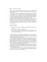
{11, 22, 30, 34, 45} {68, 69, 71, 75}
{56, 57} {82, 85, 87}
{68, 69, 71, 75, 82}
{85, 87} {45, 56, 57}
{11, 22, 30, 34}
(a) (b)
2
1

3
4
2
1
3
4
FIGURE 5.8: Distribution sorted according to (a) π =3124 and (b) π =2431.
of the best serial and parallel sorting algorithms do very poorly when applied to a
distributed environment. In this section we will examine the problem, its nature, and
its solutions.
Let us start with a clear specification of the task and its requirements. As before
in this chapter, we have a distribution D
x
1
, ,D
x
n
 of a set D among the entities
x
1
, ,x
n
of a system with communication topology G, where D
x
i
is the set of items
stored at x
i
. Each entity x
i

, because of the Distinct Identifiers assumption ID, has a
unique identity id(i), from a totally ordered sets. For simplicity, in the following we
will assume that the ids are the numbers 1, 2, ,n and that id(i) = i, and we will
denote D
x
i
simply by D
i
.
Let us now focus on the definition of a sorted distribution. A distribution is (quite
reasonably) considered sorted if, whenever i<j, all the data items stored at x
i
are
smaller than the items stored at x
j
; this condition is usually called increasing order.
A distribution is also considered sorted if all the smallest items are in x
n
, the next
ones in x
n−1
, and so on, with the largest ones in x
1
; usually, we call this condition
decreasing order. Let us be precise.
Let π be a permutation of the indices {1, ,n}. A distribution D
1
, ,D
n
 is

sorted according to π if and only if the following Sorting Condition holds:
π(i) <π(j ) ⇒∀d

∈ D
i
,d

∈ D
j
d

<d

. (5.20)
In otherwords, if the distribution issorted according to π, then allthe smallest items
must bein x
π(1)
, thenext smallestones inx
π(2)
, andso on, withthe largestones inx
π(n)
.
So the requirement that the data are sorted according to the increasing order of the ids
of the entities is given by the permutation π =12 n. The requirement of being
sorted in a decreasing order is given by the permutation π =n (n −1) 1.For
example, in Figure 5.8(b), the set is sorted according to the permutation π =2431;
in fact, all the smallest data items are stored at x
2
, the next ones in x
4

, the yet larger
ones in x
3
, and all the largest data items are stored at x
1
. We are now ready to define
the problem of sorting a distributed set.
SORTING A DISTRIBUTED SET 299
Sorting Problem Given a distribution D
1
, ,D
n
 of D and a permutation π,
the distributed sorting problem is the one of moving data items among the entities so
that, upon termination,
1. D

1
, ,D

n
 is a distribution of D, where D

i
is the final set of data at x
i
;
2. D

1

, ,D

n
 is sorted according to π.
Note that the definition does not say anything about the relationship between the
sizes of the initial sets D
i
s and those of the final sets D

i
s. Depending on which
requirement we impose, we have different versions of the problem. There are three
fundamental requirements:
invariant-sized sorting: |D
i
|=|D

i
|,1≤ i ≤ n, that is, each entity ends up with
the same number of items it started with.
equidistributed sorting: |D
π(i)
|=N/n for 1 ≤ i<n and |D
π(n)
|=N −
(n −1)N/n, that is, every entity receives the same amount of data, except
for x
π(n)
that might receive fewer items.
compacted sorting: |D

π(i)
|=min{w,N−(i −1)w}, where w ≥N/n is the
storage capacity of the entities, that is, each entity, starting from x
π(1)
, receives
as many unassigned items as it can store.
Notice that equidistributed sorting is a compacted sorting with w =N/n.For
some of the algorithms we will discuss, it does not really matter which requirement is
used; for some protocols, however, the choice of the requirement is important. In the
following, unless otherwise specified, we will use the invariant-sized requirement.
From the definition, it follows that when sorting adistributed set the relevantfactors
are the permutation according to which we sort, the topology of the network in which
we sort, the location of the entities in the network, as well as the storage requirements.
In the following two sections, we will examine some special cases that will help us
understand these factors, their interplay, and their impact.
5.3.2 Special Case: Sorting on a Ordered Line
Consider the case when we want to sort the data according to a permutation π, and
the network G is a line where x
π(i)
is connected to x
π(i+1)
,1≤ i<n. This case is
very special. In fact, the entities are located on the line in such a way that their indices
are ordered according to the permutation π. (The data, however, is not sorted.) For
this reason, G is also called an ordered line. As an example, see Figure 5.9, where
π =1, 2, ,n.
A simple sorting technique for an ordered line is OddEven-LineSort, based on the
parallel algorithm odd-even-transposition sort, which is in turn based on the well
known serial algorithm Bubble Sort. This technique is composed of a sequence of
iterations, where initially j = 0.

300 DISTRIBUTED SET OPERATIONS
{10, 15, 16} {5, 11, 14}{1, 9, 13, 18}
{3, 6, 8, 20} {2, 7, 12}
5
1234
FIGURE 5.9: A distribution on a ordered line of size n = 5.
Technique OddEven-LineSort:
1. In iteration 2j +1 (an odd iteration), entity x
2i+1
exchanges its data with neigh-
bour x
2i+2
,0≤ i ≤
n
2
−1; as a result, x
2i+1
retains the smallest items while
x
2i+2
retains the largest ones.
2. In iteration 2j (an even iteration), entity x
2i
exchanges its data with neighbour
x
2i+1
,1≤ i ≤
n
2
−1; as a result, x

2i
retains the smallest items while x
2i+1
retains the largest ones.
3. If no data items change of place at all during an iteration (other than the first),
then the process stop.
A schematicrepresentation of theoperations performed bythe technique OddEven-
LineSort is by means of the “sorting diagram”: a synchronous TED (time-event
diagram) where the exchange of data between two neighboring entities is shown
as a bold line connecting the time lines of the two entities. The sorting diagram for a
line of n = 5 entities is shown in Figure 5.10. In the diagram are clearly visible the
alternation of “odd” and “even” steps.
To obtain a fully specified protocol, we still need to explain two important opera-
tions: termination and data exchange.
Termination. We have said that we terminate when no data items change of place
at all during an iteration. This situation can be easily determined. In fact, at the end
of an iteration, each entity x can set a Boolean variable change to true or false to
indicate whether or not its data set has changed during that iteration. Then, we can
check (by computing the AND of those variables) if no data items have changed place
at all during that iteration; if this is the case for every entity, we terminate, else we
start the next iteration.
1
x
x
x
x
x
2
3
4

5
. . . .
. . . .
. . . .
. . . .
FIGURE 5.10: Diagram of operations of OddEven-LineSort in a line of size n = 5.
SORTING A DISTRIBUTED SET 301
Data Exchange. At the basis of the technique there is the exchange of data between
two neighbors, say x and y; at the end of this exchange, that we will call merge, x
will have the smallest items and y the largest ones (or vice versa). This specification
is, however, not quite precise. Assume that, before the merge, x has p items while y
has q items, where possibly p = q; how much data should x and y retain after the
merge ? The answer depends, partially, on the storage requirements.

If we are to perform a invariant-sized sorting, x should retain p items and y
should retain q items.

If we are to perform a compacted sorting, x should retain min{w, (p +q)}items
and y retain the others.

If we are to perform a equidistributed sorting, x should retain min{N/n,
p +q} items and y retain the others. Notice that, in this case each entity need
to know both n and N.
The results of the execution of OddEven-LineSort with an invariant-sized in the
sorted line of Figure 5.9 is shown in Table 5.2.
The correctness of the protocol, although intuitive, is not immediate (Exercises
5.6.23, 5.6.24, 5.6.25, and 5.6.26). In particular, the so-called “0 −1 principle” (em-
ployed to prove the correctness of the similar parallel algorithm) can not be used
directly in our case. This is due to the fact that the local data sets D
i

may contain
several items, and may have different sizes.
Cost The time cost is clearly determined by the number of iterations. In the worst
case, the data items are initially sorted the “wrong” way; that is, the initial distribution
is sorted according to permutation π

=π(n),π(n −1), ,π(1). Consider the
largest item; it has to move from x
1
to x
n
; as it can only move by one location per
iteration, to complete its move it requires n − 1 iterations. Indeed this is the actual
cost for some initial distributions (Exercise 5.6.27).
Property 5.3.1 OddEven-LineSort sorts an equidistributed distribution in n −1
iterations if the required sorting is (a) invariant-sized, or (b) equidistributed, or (c)
compacted.
TABLE 5.2: Execution of OddEven-LineSort on the System of Figure 5.9
iteration x
1
x
2
x
3
x
4
x
5
1 {1,9,13,18}→ ←{3,6,8,20}{2,7,12}→ ←{10,15,16}{5,11,14}
2 {1,3,6,8}{9,13,18,20}→ ←{2,7,10}{12,15,16}→ ←{5,11,14}

3 {1,3,6,8}→ ←{2,7,9,10}{13,18,20}→ ←{5,11,12}{14,15,16}
4 {1,2,3,6}{7,8,9,10}→ ←{5,11,12}{13,18,20}→ ←{14,15,16}
5 {1,2,3,6}→ ←{5,7,8,9}{10,11,12}→ ←{13,14,15}{16,18,20}
6 {1,2,3,5}{6,7,8,9}→ ←{10,11,12}{13,14,15}→ ←{16,18,20}
302 DISTRIBUTED SET OPERATIONS
Interestingly, the number of iterations can actually be much more than n −1ifthe
initial distribution is not equidistributed.
Consider, for example, an invariant-sized sorting when the initial distribution is
sorted according to permutation π

=π(n),π(n −1), ,π(1). Assume that x
1
and x
n
have each kq items, while x
2
has only q items. All the items initially stored
in x
1
must end up in x
n
; however, in the first iteration only q items will move from
x
1
to x
2
; because of the “odd-even” alternation, the next q items will leave x
1
in the
3rd iteration, the next q in the 5th, and so on. Hence, the total number of iterations

required for all data to move from x
1
to x
n
is at least n −1 +2(k −1). This implies
that, in the worst case, the time costs can be considerably high (Exercise 5.6.28):
Property 5.3.2 OddEven-LineSort performs an invariant-sized sorting in at most
N − 1 iterations. This number of iterations is achievable.
Assuming (quite unrealistically) that the entire data set of an entity can be sent in
one time unit to its neighbor, the time required by all the merge operations is exactly
the same as the number of iterations. In contrast to this, to determine termination,
we need to compute the AND of the Boolean variables change at each iteration. This
operation can be done on a line in time n −1 at each iteration. Thus, in the worst
case,
T[OddEven −LineSort
invariant
] = O(nN). (5.21)
Similarly, bad time costs can be derived for equidistributed sorting and compacted
sorting.
Let us focus now on the number of messages for invariant-sized sorting. If we
do not impose any size constraints on the initial distribution then, by Property 5.3.2,
the number of iterations can be as bad as N −1; as in each iteration we perform the
computation of the function AND, and this requires 2(n −1) messages, it follows
that the protocol will use
2(n −1)(N −1)
messages just for computing the AND. To this cost we still need to add the number
of messages used for the transfer of data items. Hence, without storage constraints
on the initial distribution, the protocol has a very high cost due to the high number of
iterations possible.
Let us consider now the case when the initial distribution is equidistributed. By

property 5.3.1,the number ofiterations is atmost n − 1 (instead ofN −1). Thismeans
that the cost of computing the AND is O(n
2
) (instead of O(Nn)). Surprisingly, even
in this case, the total number of messages can be very high.
Property 5.3.3 OddEven-LineSort can use O(Nn) messages to perform an
invariant-sized sorting. This cost is achievable even if the data is initially equidis-
tributed.
SORTING A DISTRIBUTED SET 303
To see why this is the case, consider an initial equidistribution sorted according
to permutation π

=π(n),π(n −1), ,π(1). In this case, every data item will
change location in each iteration (Exercise 5.6.29), that is, O(N) messages will be
sent in each iteration. As there can be n −1 iterations with an initial equidistribution
(by Property 5.3.1), we obtain the bound. Summarizing:
M[OddEven −LineSort]
invariant
= O(nN). (5.22)
That is, using Protocol OddEven-LineSort can costs as much as broadcasting all
the data to every entity. This results holds even if the data is initially equidistributed.
Similar bad message costs can be derived for equidistributed sorting and compacted
sorting.
Summarizing, Protocol OddEven-LineSort does not appear to be very efficient.
IMPORTANT. Each line network is ordered according to a permutation. However,
this permutation might not be π, according to which we need to sort the data. What
happens in this case?
The protocol OddEven-LineSort does not work if the entities are not positioned
on the line according to π, that is, when the line is not ordered according to π.
(Exercise 5.6.30). The question then becomes how to sort a set distributed on an

unsorted line. We will leave this question open until later in this chapter.
5.3.3 Removing the Topological Constraints: Complete Graph
One of the problems we have faced in the the line graph is the constraint that the
topology of the network imposes. Indeed, the line graph is one of the worst topologies
for a tree, as its diameter is n − 1. In this section we will do the opposite: We will
consider the complete graph, where every entity is directly connected to every other
entity; in this way, we will be able to remove the constraints imposed by the network
topology. Without loss of generality (since we are in a complete network), we assume
π =1, 2, ,n.
As the complete graph contains every graph as a subgraph, we can choose to
operate on whichever graph suites best our computational needs. Thus, for example,
we can choose an ordered line and use protocol OddEven-LineSort we discussed
before. However, as we have seen, this protocol is not very efficient.
If we are in a complete graph, we can adapt and use some of the well known
techniques for serial sorting.
Let us focus on the classical Merge-Sort strategy. This strategy, in our distributed
setting becomesas follows:(1) thedistribution tobe sorted isfirst dividedin twopartial
distributions of equal size; (2) each of these two partial distribution is independently
sorted recursively using MergeSort; and (3) then the two sorted partial distributions
are merged to form a sorted distribution.
The problemwith thisstrategy isthat thelast step,the mergingstep, isnot an obvious
one in a distributed setting; in fact, after the first iteration, the two sorted distributions
304 DISTRIBUTED SET OPERATIONS
to be merged are scattered among many entities. Hence the question: How do
we efficiently “merge” two sorted distributions of several sets to form a sorted
distribution?
There are many possible answers, each yielding a different merge-sort protocol.
In the following we discuss a protocol for performing distributed merging by means
of the odd-even strategy we discussed for the ordered line.
Let us first introduce some terminology. We are given a distribution D =

D
1
, ,D
n
. Consider now a subset {D
j
1
, ,D
j
q
} of the data sets, where j
i
<
j
i+1
(1 ≤ i ≤ q). The corresponding distribution D

=D
j
1
, ,D
j
q
 is called a
partial distribution of D. We say that the partial distribution d

is sorted (according to
π =1, ,n) if all the items in D
j
i

are smaller that the items in D
j
i+1
,1≤ i<q.
Note that it might happen that D

is sorted while D is not.
Let us now describe how to odd-even-merge a sorted partial distribution
A
1
, ,A
p
2
 with a sorted partial distribution A
p
2
+1
, ,A
p
 to form a sorted
distributionA
1
, ,A
p
, where we are assuming forsimplicity that p is apower of 2.
OddEven-Merge Technique:
1. If p = 2, then there are two sets A
1
and A
2

, held by entities y
1
and y
2
, respec-
tively. To odd-even-merge them, each of y
1
and y
2
sends its data to the other
entity; y
1
retains the smallest while y
2
retains the largest items. We call this
basic operation simply merge.
2. If p>2, then the odd-even-merge is performed as following:
(a) first recursively odd-even-merge the distribution A
1
,A
3
,A
5
, ,A
p
2
−1

with the distribution A
p

2
+1
,A
p
2
+3
,A
p
2
+5
, ,A
p−1
;
(b) then recursively odd-even-merge the distribution A
2
,A
4
,A
6
, ,A
p
2

with the distribution A
p
2
+2
,A
p
2

+4
,A
p
2
+6
, ,A
p
;
(c) finally, merge A
2i
with A
2i+1
(1 ≤ i ≤
p
2
−1)
The technique OddEven-Merge can then be used to generate the OddEven-MergeSort
technique for sorting a distribution D
1
, ,D
n
. As in the classical case, the
technique is defined recursively as follows:
OddEven-MergeSort Technique:
1. recursively odd-even-merge-sort the distribution D
1
, ,D
n
2
 ,

2. recursively odd-even-merge-sort the distribution D
n
2
+1
, ,D
n

3. odd-even-merge D
1
, ,D
n
2
 with D
n
2
+1
, ,D
n

Using this technique, we obtain a protocol for sorting a distribution D
1
, ,D
n
;
we shall call this protocol like the technique itself: Protocol OddEven-MergeSort.
To determine the communication costs of this protocol need to “unravel” the
recursion.
SORTING A DISTRIBUTED SET 305
1
x

6
x
7
x
8
x
x
x
x
x
2
3
4
5
FIGURE 5.11: Diagram of operations of OddEven-MergeSort with n = 8.
When we do this, we realize that the protocol is a sequence of 1 +log n iterations
(Exercise 5.6.32). In each iteration (except the last) every entity is paired with another
entity, and each pair will perform a simple merge of their local sets; half of the entities
will perform this operation twice during an iteration. In the last iteration all entities,
except x
1
and x
n
, will be paired and perform a merge.
Example Using the sorting diagram to describe these operations, the structure of
an execution of Protocol OddEven-MergeSort when n = 8 is shown in Figure 5.11.
Notice that there are 4 iterations; observe that, in iteration 2, merge will be
performed between the pairs (x
1
,x

3
), (x
2
,x
4
), (x
5
,x
7
), (x
6
,x
8
); observe further that
entities x
2
,x
3
,x
6
,x
7
will each be involved in one more merge in this same iteration.
Summarizing, in each of the first log n iterations, each entity sends is data to one or
two other entities. In other words the entire distributed set is transmitted in each itera-
tion. Hence, the total number of messages used by Protocol OddEven-MergeSort is
M[OddEven −MergeSort] = O(N log n). (5.23)
Note that this bound holds regardless of the storage requirement.
IMPORTANT. Does the protocol work ? Does it in fact sorts the data ? The answer
to these questions is: not always. In fact, its correctness depends on several factors,

including the storage requirements.
It is not difficult to prove that the protocol correctly sorts, regardless of the storage
requirement, if the initial set is equidistributed (Exercise 5.6.33).
306 DISTRIBUTED SET OPERATIONS
1
x
x
2
x
3
x
4
{4, 8} {1, 4}
{6} {3}
{7} {6} {6}
{1, 3} {3, 7} {7, 8} {7, 8}
{1, 4}
{3}{8}
{4, 6}
{1}
FIGURE 5.12: OddEven-MergeSort does not correctly perform an invariant sort for this
distribution.
Property 5.3.4 OddEven-MergeSort sorts any equidistributed set if the required
sorting is (a) invariant-sized, (b) equidistributed, or (c) compacted.
However, if the initial set is not equidistributed, the distribution obtained when
the protocol terminates might not be sorted. To understand why, consider performing
an invariant sorting in the system of n = 4 entities shown in Figure 5.12; items 1
and 3, initially at entity x
4
, should end up in entity x

1
, but item 3 is still at x
4
when
the protocol terminates. The reason for this happening is the “bottleneck” created
by the fact that only one item at a time can be moved to each of x
2
and x
3
. Recall
that the existence of bottlenecks was the reason for the high number of iterations of
Protocol OddEven-LineSort. In this case, the problem makes the protocol incorrect. It
is indeed possible to modify the protocol, adding enough appropriate iterations, so that
the distribution will be correctly solved. The type and the number of the additional
iterations needed to correct the protocol depends on many factors. In the example
shown in Figure 5.12, a single iteration consisting of a simple merge between x
1
and
x
2
would suffice. In general, the additional requirements depend on the specifics of
the size of the initial sets; see, for example, Exercise 5.6.34.
5.3.4 Basic Limitations
In the previous sections we have seen different protocols, examined their behavior,
and analyzed their costs. In this process we have seen that the amount of data items
transmitted can be very large. For example, in OddEven-LineSort the number of
messages is O(Nn), the same as sending every item everywhere. Even not worrying
about the limitations imposed by the topology of the network, protocol OddEven-
MergeSort still uses O(N logn) messages when it works correctly. Before proceeding
any further, we are going to ask the following question: How many messages need to

be sent anyway? we would like the answer to be independent of the protocol but to
take into account both the topology of the network and the storage requirements. The
purpose of this section is to provide such an answer, to use it to assess the solutions
seen so far, and to understand its implications. On the basis of this, we will be able to
design an efficient sorting protocol.
Lower Bound There is a minimum necessary amount of data movements that
must take place when sorting a distributed set. Let us determine exactly what costs
must be incurred regardless of the algorithm we employ.
SORTING A DISTRIBUTED SET 307
The basic observation we employ is that, once we are given a permutation π
according to which we must sort the data, there are some inescapable costs. In fact, if
entity x has some data that according to π must end up in y, then this data must move
from x to y, regardless of the sorting algorithm we use. Let us state these concepts
more precisely.
Given a network G, a distribution D =D
1
, ,D
n
of Don G, and a permutation
π let D

=D

1
, ,D

n
 be the result of sorting D according to π . Then |D
i
∩D


j
|
items must travel from x
i
to x
j
; this means that the amount of data transmission for
this transfer is at least
|D
i
∩D

j
| d
G
(x
i
,x
j
).
How this amount translates into number of messages depends on the size of the
messages. A message can only contain a (small) constant number of data items; to
obtain a uniform measure, we consider just one data item per message. Then
Theorem 5.3.1 The number of messages required to sort D according to π inGis
at least
C(D,G,π) =

i=j
|D

i
∩D

j
| d
G
(x
i
,x
j
).
This expresses a lower bound on the amount of messages for distributed sorting;
the actual value depends on the topology G and the storage requirements. The deter-
mination of this value in specific topologies for different storage requirements is the
subject of Exercises 5.6.35–5.6.38.
Assessing Previous Solutions Let us see what this bound means for situations
we have already examined. In this bound, the topology of the network plays a role
through the distances d
G
(x
i
,x
j
) between the entities that must transfer data, while
the storage requirements play a role through the sizes |D

i
| of the resulting sets.
First of all, note that, by definition, for all x
i

,x
j
,wehave
d
G
(x
i
,x
j
) ≤ d(G);
furthermore,

i=j
|D
i
∩D

j
|≤ N. (5.24)
To derive lower bounds on the number of messages for a specific network G,we
need to consider for that network the worst possible allocation of the data, that is, the
one that maximizes C(D,G,π).
Ordered Line. OddEven-LineSort
Let us focus first on the ordered line network.
308 DISTRIBUTED SET OPERATIONS
If the data is not initially equidistributed, it easy to show scenarios where O(N)
data must travel a O(n) distance along the line. For example, consider the case when
x
n
initially contains the smallest N −n +1 items while all other entities have just

a single item each; for simplicity, assume (N −n +1)/n to be integer. Then for
equidistributed sorting we have |D
n
∩D

j
|=(N − n +1)/n for j<n; this means
that at least

j<n
|D
n
∩D

j
| d
G
(x
n
,x
j
) =

j<n
j (N − n +1)/n = ⍀(nN)
messages are needed to send the data initially in x
n
to their final destinations. The
same example holds also in the case of compact sorting.
In the case of invariant sorting, surprisingly, the same lower bound exists even

when the data is initially equidistributed; for simplicity, assume N/n to be integer
and n to be even. In this case, in fact, the worst initial arrangement is when the
data items are initially sorted according to the permutation 
n
2
+1,
n
2
+2, ,n−1,
n, 1, 2, ,
n
2
−1,
n
2
, while we want to sort them according to π =1, 2, ,n.
In this case we have that all the items initially stored at x
i
,1≤ i ≤ n/2, must end
up in x
n
2
+i
, and vice versa, that is, D

i
= D
n
2
+i

. Furthermore, in the ordered line,
d(x
i
,x
n
2
+i
) =
n
2
,1≤ i ≤ n/2. This means that each item must travel distance
n
2
.
That is the total amount of communication must be at least

i=j
|D
i
∩D

j
| d
G
(x
i
,x
j
) =
n

2
N = ⍀(nN ).
Summarizing, in the ordered line, regardless of the storage requirements, ⍀(nN )
messages need to be sent in the worst case.
This facthas a surprising consequence.It implies that the complexity of thesolution
for the ordered line, protocolOddEven-LineSort, was not bad after all. Onthe contrary,
protocol protocol OddEven-LineSort is worst-case optimal.
Complete Graph. OddEven-MergeSort
Let us turn to the complete graph. In this graph d
G
(x
i
,x
j
) = 1 for any two distinct
entities x
i
and x
j
. Hence, the lower bound of Theorem 5.3.1 in the complete graph
K becomes simply
C(D,K,π) =

i=j
|D
i
∩D

j
|. (5.25)

This means that, by relation 5.24, in the complete graph no more than N messages
need to be sent in the worst case. At the same time, it is not difficult to find, for each
type of storage requirement, a situation where this lower bound becomes ⍀(N), even
when the set is initially equidistributed (Exercise 5.6.35).
SORTING A DISTRIBUTED SET 309
In other words, the number of messages that need to be sent in the worst case is
no more and no less than ⍀(N).
By Contrast, we have seen that protocol OddEven-MergeSort always uses
O(N log N) messages; thus, there is a large gap between upper bound and lower
bound. This indicates that protocol OddEven-MergeSort, even when correct, is far
from optimal.
Summarizing, the expensive OddEven-LineSort is actually optimal for the ordered
line, while OddEven-MergeSort is far from being optimal in the complete graph.
Implications for Solution Design The bound of Theorem 5.3.1 expresses a
cost that every sorting protocol must incur. Examining this bound, there are two
considerations that we can make.
The first consideration is that, to design an efficient sorting protocol, we should
not worry about this necessary cost (as there is nothing we can do about it), but
rather focus on reducing the additional amount of communication. We must, however,
understand that the necessary cost is that of the messages that move data items to their
final destination (through the shortest path). These messages are needed anyway; any
other message is an extra cost, and we should try to minimize these.
The second consideration is that, as the data items must be sent to their final
destinations, we could use the additional cost just to find out what the destinations
are. This simple observation leads to the following strategy for a sorting protocol, as
described from the individual entity point of view:
Sorting Strategy
1. First find out where your data items should go.
2. Then send them there through the shortest-paths.
The second step is the necessary part and causes the cost stated by Theorem 5.3.1.

The first step is the one causing extra cost. Thus, it is an operation we should perform
efficiently.
Notice that there are many factors at play when determining where the final desti-
nation of a data item should be. In fact, it is not only due to the permutation π but also
to factors such as which final storage requirement is imposed, for example, on whether
the final distribution must be invariant-sized, or equidistributed, or compacted.
In the following section we will see how to efficiently determine the final destina-
tion of the data items.
5.3.5 Efficient Sorting: SelectSort
In this section our goal is to design an efficient sorting protocol using the strategy
of first determining the final destination of each data item, and only then moving the
items there. To achieve this goal, each entity x
i
has to efficiently determine the sets
D
i
∩D

π(j)
,
310 DISTRIBUTED SET OPERATIONS
that is, which of its own data items must be sent to x
π(j)
,1≤ j ≤ n. How can this be
done ? The answer is remarkably simple.
First observe that the final destination of a data item (and thus the final distribution
D

) depends on the permutation π as well as on the final storage requirement. Different
criteria determine different destinations for the same data item. For example, in the

ordered line graph of Figure 5.9, the final destination of data item 16 is x
5
in an
invariant-sized final distribution; x
4
in an equidistributed final distribution; and x
3
in
an compacted final distribution with storage capacity w = 5.
Although the entities do not know beforehand the final distribution, once they
know π and the storage requirement used, they can find out the number
k
j
=|D

π(j)
|
of data items that must end up in each x
π(j)
.
Assume for the moment that the k
j
s are known to the entities. Then, each x
i
knows
that D

π(1)
at the end must contain the k
1

smallest data items; D

π(2)
at the end must
contain the next k
2
smallest, etc., and D

π(n)
at the end must contain the k
n
largest
item. This fact has an immediate implication.
Let b
1
= D[k
1
]bethek
1
th smallest item overall. As x
π(1)
must contain in the end
the k
1
smallest items, then all the items d ≤ b
1
must be sent to x
π(1)
. Similarly, let
b

j
= D[

l≤j
k
l
] be the (k
1
+ +k
j
)th smallest item overall; then all the items d
with b
j−1
<d≤ b
j
must be sent to x
π(j)
. In other words,
D
i
∩D

π(j)
={d ∈ D
i
: b
j−1
<d≤ b
j
}.

Thus, to decide the final destination of its own data items, each x
i
needs only to
know the values of items b
1
,b
2
, b
n
. To determine each of these values we just need
to solve a distributed selection problem, whose solution protocols we have discussed
earlier in this chapter.
This gives raise to a general sorting strategy, that we shall call SelectSort, whose
high-level description is shown in Figure 5.13. This strategy is composed of n −1
iterations. Iteration j ,1≤ j ≤ n −1 is started by x
π(j)
and it is used to determine
at each entity x
i
which of its own items must be eventually sent to x
π(j)
(i.e., to
determine D
i
∩D

π(i)
). More precisely:
1. The iteration starts with x
π(j)

broadcasting the number k
j
of items that, accord-
ing to the storage requirements, it must end up with.
2. The rest of the iteration then consists of the distributed determination of the
k
j
th smallest item among the data items still under consideration (initially, all
data items are under consideration).
3. The iterations terminates with the broadcast of the found item b
j
: Upon receiv-
ing it, each entity y determines, among the local items still under consideration,
those that are smaller or equal to b
1
; x
i
then assigns x
π(j)
to be the destination
for those items, and removes them from consideration.
SORTING A DISTRIBUTED SET 311
Strategy SelectSort
begin
for j = 1, ,n−1 do
Collectively determine b
j
= D[k
j
] using distributed

selection;
* Assign destination: 
D
i,j
:={d ∈ D
i
: b
j−1
<d≤ b
j
};
endfor
D
i,n
:={d ∈ D
i
: b
n−1
<d};
for j = 1, ,n−1 do
* Send all data items to their final destination: 
send D
i,j
to x
π(j)
;
endfor
end
FIGURE 5.13: Strategy SelectSort.
At theend of the (n −1)th iteration,each entity x

i
assigns x
π(n)
to bethe destination
for any local item still under consideration. At this point, the final destination of each
data item has been determined; thus, they can be sent there.
To transform this technique into a protocol, we need to add a final step in which
each entity sends the data to their discovered destinations. We also need to ensure that
x
π(j)
knows k
j
at the beginning of the jth iteration; fortunately, this condition is easy
to achieve (Exercise 5.6.39). Finally, we must specify the protocol used for distributed
selection in the iterations. If we choose protocol ReduceSelect we have discussed in
Section 5.2.5, we will call the resulting sorting algorithm Protocol SelectSort (see
Exercise 5.6.40).
IMPORTANT. Unlike the other two sorting protocols we have examined, Protocol
SelectSort is generic, that is, it works in any network, regardless of its topology.
Furthermore, unlike OddEven-MergeSort, it always correctly sorts the distribution.
To determine the cost of protocol SelectSort, first observe that both the initial and
the final broadcast of each iteration can be integrated in the execution of ReduceSelect
in that iteration; hence, the only additional cost of these protocols (i.e., the cost to
find the final destination of each data item) is solely due to the n −1 executions of
ReduceSelect. Let us determine these additional cost.
Let M[K,N] denote the number of messages used to determine the kth smallest
out of a distributed set of N elements. As we have chosen protocol ReduceSelect,
then ( recall expression 5.18) we have
M[K,N] = log(min{K, N −K +1})M[Rank] +l.o.t.
where M[Rank] is the number of messages required to select in a small set.

Let K
i
=

j≤i
k
j
. Then, the total additional cost of the resulting protocol
312 DISTRIBUTED SET OPERATIONS
SelectSort is

1≤i≤n−1
M[k
i
,N −K
i−1
] = M[Rank]

1≤i≤n−1
log(min{k
i
,N −K
i
+1}) +l.o.t
(5.26)
IMPORTANT. Notice that M[Rank] is a function of n only, whose value depends
on the topology of the network G, but does not depend on N. Hence the additional
cost of the protocol SelectSort is always of the form O(f
G
(n) log N)). So as long as

this quantity is of the same order (or smaller) than the necessary cost for G, protocol
SelectSort is optimal.
For example, in the complete graph we have that M[Rank] = O(n). Thus,
Expression 5.26 becomes O(n
2
log N/n). Recall (Equation 5.25) that the necessary
cost in a complete graph is at most N . Thus, protocol SelectSort is optimal, with to-
tal cost (necessary plus additional) of O(N), whenever N>>n, for example, when
N ≥ n
2
log n. In contrast, protocol OddEven-MergeSort has always worst-case cost
of O(N log n), and it might even not sort.
The determination of the cost of protocol SelectSort in specific topologies for
different storage requirements is the subject of Exercises 5.6.41–5.6.48.
5.3.6 Unrestricted Sorting
In the previous section we have examined the problem of sorting a distributed set
according to a given permutation. This describes the common occurrence when there
is some a priori ordering of the entities (e.g., of their ids), according to which the data
must be sorted.
There are, however, occurrences where the interest is to sort the data with no a
priori restriction on what ordering of the sites should be used. In other words, in these
cases, the goal is to sort the data according to a permutation. This version of the
problem is called unrestricted sorting.
Solving the unrestricted sorting problem means that we, as designers, have the
choice of the permutation according to which we will sort the data. Let us examine
the impact of this choice in some details.
We have seen that, for a given permutation π, once the storage requirement is
fixed, there is an amount of message exchanges that must necessarily be performed to
transfer the records to their destinations; this amount is expressed by Theorem 5.3.1.
Observe that this necessary cost is smaller for some permutations than for others.

For example, assume that the data is initially equidistributed sorted according to
π
1
=1, 2, ,n, where n is even. Obviously, there is no cost for an equidistributed
sorting of the set according to π
1
, as the data is already in the proper place.By contrast,
if we need to sort the distribution according to π
2
=n, n −1, ,2, 1, then, even
with the same storage requirement as before, the operation will be very costly: At
least N messages must be sent, as every data item must necessarily move.