Orr, F. M. - Theory of Gas Injection Processes Episode 14 doc
Bạn đang xem bản rút gọn của tài liệu. Xem và tải ngay bản đầy đủ của tài liệu tại đây (219.84 KB, 20 trang )
Bibliography 251
[90] Orr, F.M., Jr. and Taber J.J. Use of Carbon Dioxide in Enhanced Oil Recovery. Science,
page 563, 11 May 1984.
[91] Orr, F.M., Jr., Dindoruk, B., and Johns, R.T. Theory of Multicomponent Gas/Oil Displace-
ments. Ind. Eng. Chem. Res., 34:2661–2669, 1995.
[92] Orr, F.M., Jr., Johns, R.T. and Dindoruk, B. Development of Miscibility in Four-Component
CO
2
Floods. Soc. Pet. Eng. Res. Eng., 8:135–142, 1993.
[93] Orr, F.M. Jr., Silva, M.K., Lien, C.L. and Pelletier, M.T. Laboratory Experiments to Evaluate
Field Prospects for Carbon Dioxide Flooding. J. Pet. Tech., pages 888–898, April 1982.
[94] Orr, F.M., Jr., Yu, A.D., and Lien, C.L. Phase Behavior of CO
2
and Crude Oil in Low-
Temperature Reservoirs. Society of Petroleum Engineers Journal, pages 480–492, August
1981.
[95] Pande, K.K. Interaction of Phase Behaviour with Nonuniform Flow. PhD thesis, Stanford
University, Stanford, CA, December 1988.
[96] Peaceman, D.W. Fundamentals of Numerical Reservoir Simulation. Elsevier Scientific Pub-
lishing, New York, 1977.
[97] Pedersen, K.S., Fjellerup, J.F., Fredenslund, A., and Thomassen, P. Studies of Gas Injection
into Oil Reservoirs by a Cell to Cell Simulation Model, SPE 13832, 1985.
[98] Pedersen, K.S., Fredenslund, A., and Thomassen, P. Properties of Oils and Natural Gases.
Gulf Publishing Company, Houston, Texas, 1989.
[99] Peng, D.Y. and Robinson, D.B. A New Two-Constant Equation of State. Ind. Eng. Chem.
Fund., 15:59–64, 1976.
[100] Perkins, T.K.and Johnston, O.C. A Review of Diffusion and Dispersion in Porous Media.
Soc. Pet. Eng. J., pages 70–84, March 1963.
[101] Pope, G.A. The Application of Fractional Flow Theory to Enhanced Oil Recovery. Soc. Pet.
Eng. J., 20:191–205, June 1980.
[102] Pope, G.A., Lake, L.W. and Helfferich, F.G. Cation Exchange in Chemical Flooding: Part 1
- Basic Theory Without Dispersion. Soc. Pet. Eng. J., pages 418–434, December 1978.
[103] Ratchford, HH. and Rice, J.D. Procedure for Use of Electrical Digital Computers in Cal-
culating Flash Vaporization Hydrocarbon Equilibrium. J. Pet. Tech., pages 19–20, October
1952.
[104] Reamer, H.H. and Sage, B.H. Phase Equilibria in Hydrocarbon Systems. Volumetric and
Phase Behavior of the n-Decane–CO
2
System. J. Chem. Eng. Data, 8(4):508–513, October
1963.
[105] Reid, R.C., Prausnitz, J.M., and Sherwood, T.K. The Properties of Gases and Liquids, 3rd
ed. McGraw Hill, New York, NY, 1977.
252 Bibliography
[106] Rhee, H., Aris, R. and Amundson, N.R. First-Order Partial Differential Equations: Volume
I. Prentice-Hall, Englewood Cliffs, NJ, 1986.
[107] Rhee, H., Aris, R. and Amundson, N.R. First-Order Partial Differential Equations: Volume
II. Prentice-Hall, Englewood Cliffs, NJ, 1989.
[108] Rhee, H.K., Aris, R., and Amundson, N.R. On the Theory of Multicomponent Chromatog-
raphy. Phil. Trans. Roy. Soc. London, 267 A:419–455, 1970.
[109] Seto, C.J., Jessen, K., and Orr, F.M., Jr. Compositional Streamline Simulation of Field Scale
Condensate Vaporization by Gas Injection, SPE 79690, SPE Reservoir Simulation Sympo-
sium, Houston, TX, February 3–5 2003.
[110] Shaw, J. and Bachu, S. Screening, Evaluation , and Ranking of OIl Reservoirs Suitable for
CO
2
-Flood EOR and Carbon Dioxide Sequestration. J. Canadian Pet. Tech., 41 (9):51–61,
2002.
[111] Slattery, J.C. Momentum, Energy, and Mass Transfer in Continua. McGraw-Hill, New York,
NY, 1972.
[112] Stalkup, F.I. Miscible Displacement. Society of Petroleum Engineers, Dallas, 1983.
[113] Stalkup, F.I. Miscible Displacement. Monograph 8, Soc. Pet. Eng. of AIME, New York, 1983.
[114] Stalkup, F.I. Displacement Behavior of the Condensing/Vaporizing Gas Drive Process, SPE
16715, SPE Annual Technical Conference and Exhibition, Dallas, TX, September 1987.
[115] Stalkup, F.I. Effect of Gas Enrichment and Numerical Dispersion on Enriched-Gas-Drive
Predictions. Soc. Pet. Eng. Res. Eng., pages 647–655, November 1990.
[116] Stein, M.H., Frey, D.D., Walker, R.D., and Pariani, G.J. Slaughter Estate Unit CO
2
Flood:
Comparison between Pilot and Field Scale Performance. J. Pet. Tech., pages 1026–1032,
September 1992.
[117] Taber, J.J., Martin, F.D., and Seright, R.D. EOR Screening Critera Revisited–Part I: In-
troduction to Screening Criteria and Enhanced Recovery Field Projects. Soc. Pet. Eng. Res.
Eng., pages 189–198, August 1997.
[118] Tanner, C.S., Baxley, P.T., Crump, J.G., and Miller, W.C. Production Performance of the
Wasson Denver Unit CO
2
Flood, SPE 24156, SPE/DOE 8th Annual Symposium on Enhanced
Oil Recovery, Tulsa, OK, April 22-24 1992.
[119] Thiele, M.R. Modeling Multiphase Flow in Heterogeneous Media Using Streamtubes.PhD
thesis, Stanford University, Stanford, CA, December 1994.
[120] Thiele, M.R., Batycky, R.P., and Blunt, M.J. A Streamline-Based 3D Field-Scale Composi-
tional Simulator, SPE 38889, SPE Annual Technical Conference and Exhibition, San Antonio,
TX, October 5-8 1997.
[121] Thiele, M.R., Blunt, M.J., and Orr, F.M., Jr. Modeling Flow in Heterogeneous Media Using
Streamlines–II. Compositional Displacements. In Situ, 19(4):367–391, 1995.
Bibliography 253
[122] van der Waals, J.D. On the Continuity of the Gaseous and Liquid States. In J.S. Rowlinson,
editor, J.D van der Waals: On the Continuity of the Gaseous and Liquid States, pages 83–140.
North-Holland Physics Publishing, 1988.
[123] Van Ness, H.C. and Abbott, M.M. Classical Thermodynamics of Nonelectrolyte Solutions
With Applications to Phase Equilibrium. McGraw-Hill, San Francisco, 1982.
[124] Varotsis, N., Stewart, G., Todd, A.C. and Clancy, M. Phase Behavior of Systems Comprising
North Sea Reservoir Fluids and Injection Gases. J. Pet. Tech., pages 1221–1233, November
1986.
[125] Wachmann, C. The Mathematical Theory for the Displacement of Oil and Water by Alcohol.
Society of Petroleum Engineers Journal, 231:250–266, September 1964.
[126] Walas, S.M. Phase Equilibria in Chemical Engineering. Butterworth Publishers, Stoneham,
MA, 1985.
[127] Walsh, B.W. and Orr, F.M. Jr. Prediction of Miscible Flood Performance: The Effect Of
Dispersion on Composition Paths in Ternary Systems. IN SITU, 14(1):19–47, 1990.
[128] Wang, Y. Analytical Calculation of Minimum Miscibility Pressure. PhD thesis, Stanford
University, Stanford, CA, 1998.
[129] Wang, Y. and Orr, F.M., Jr. Analytical Calculation of Minimum Miscibility Pressure. Fluid
Phase Equilibria, 139:101–124, 1997.
[130] Wang, Y. and Orr, F.M., Jr. Calculation of Minimum Miscibility Pressure. J. Petroleum
Science and Engineering, 27:151–164, 2000.
[131] Wang, Y., and Peck, D.G. Analytical Calculation of Minimum Miscibility Pressure: Com-
prehensive Testing and Its Application in a Quantitative Analysis of the Effect of Numerical
Dispersion for Different Miscibility Development Mechanisms, SPE 59738, SPE/DOE Im-
proved Oil Recovery Symposium, Tulsa, OK, April 2000.
[132] Watkins, R.W. A Technique for the Laboratory Measurement of Carbon Dioxide Unit Dis-
placement Efficiency in Reservoir Rock, SPE 7474, SPE Annual Technical Conference and
Exhibition, Dallas, TX, Oct. 1-3 1978.
[133] Welge, H.J. A Simplified Method for Computing Oil Recovery by Gas or Water Drive. Trans.,
AIME, 195:91–98, 1952.
[134] Welge, H.J., Johnson, E.F., Ewing, S.P.,Jr., and Brinkman, F.H. The Linear Displacement
of Oil from Porous Media by Enriched Gas. J. Pet. Tech., pages 787–796, August 1961.
[135] Whitson, C.H. and Michelsen, M. The Negative Flash. Fluid Phase Equilibria, 53:51–71,
1989.
[136] Wilson, G.M. A Modified Redlich-Kwong Equation of State, Application to General Physical
Data Calculation. Paper 15C, presented at the 1969 AIChE 65th National Mtg., Cleveland,
OH, 1969.
254 Bibliography
[137] Wingard, J.S. Multicomponent, Multiphase Flow in Porous Media with Temperature Varia-
tion. PhD thesis, Stanford University, Stanford, CA, November 1988.
[138] Yellig, W.F., and Metcalfe, R.S. Determination and Prediction of CO
2
Minimum Miscibility
Pressures. J. Pet. Tech., pages 160–168, January 1980.
[139] Zhu, J., Jessen, K., Kovscek, A.R., and Orr, F.M., Jr. Analytical Theory of Coalbed Methane
Recovery by Gas Injection. Soc. Pet. Eng. J., pages 371–379, December 2003.
[140] Zick, A.A. A Combined Condensing/Vaporizing Mechanism in the Displacement of Oil by
Enriched Gas, SPE 15493, SPE Annual Technical Conference and Exhibition, New Orleans,
LA, October 1986.
Appendix A 255
APPENDIX A: Entropy Conditions in Ternary Systems
In this appendix we consider the entropy condition for shocks in ternary systems. The derivation
of the entropy condition for the shock between tie lines follows that of Wang [128], which is based,
in turn, on the approach used by Johansen and Winther [51] to study polymer displacements. The
derivation given here is for a specific system with constant K-values, but the patterns of behavior
are the same for systems with variable K-values. The use of the constant K-value example is an
attempt to illustrate the abstract concept of an entropy condition in a concrete way.
Entropy conditions are statements about the stability of a shock, written in terms of the relative
magnitudes of eigenvalues of compositions on either side of the shock and the shock velocity. If a
shock is stable, it must be self-sharpening. In other words, if a stable shock were to be smeared
slightly by some physical mechanism, it must sharpen again into a shock in the limit as that physical
mechanism is removed. Dispersion is one physical mechanism that can create a continuously varying
composition in place of a jump in composition. In a binary displacement, the requirement of a stable
shock can be translated easily into a statement about the eigenvalues on either side of the shock.
For example, the discussion in Section 4.2 states that the eigenvalue on the upstream side of a
shock must be greater than the shock velocity, and the eigenvalue on the downstream side must be
less than the shock velocity. For a ternary displacement, however, there are two eigenvalues at each
point in the composition space, so the statement of shock stability in terms of those eigenvalues is
necessarily more complex. In this appendix we consider the statement of an entropy condition for
each of the shocks that can appear in the solution for a ternary displacement, leading, trailing, and
intermediate, and we show that if there is an intermediate shock, it is a semishock.
Leading Shock
To illustrate the statement of the entropy condition for the various shocks, we consider a specific
case: constant K-values, with K
1
=2.5,K
2
=0.5,K
3
= 0.05, and M = 5. The solution for this
example is shown in Fig. 5.16. The behavior of the leading shock, which connects a single-phase
composition with a composition on the initial tie line, is exactly the same as that described for
leading shock in a binary system (see Section 4.2). The leading shock is a shock that arises because
of the behavior of λ
t
, and it occurs along the extension of the initial tie line. It is a semishock that
is faster than the composition velocities on the downstream side of the shock, the right state for
this shock (entropy conditions are frequently written in terms of left and right states, with the left
state referring to upstream compositions and the right state to downstream compositions). Those
velocities are are all one. Fig. A.1 shows the relationships between the shock velocity and the
eigenvalues λ
t
and λ
nt
for the leading shock. The leading shock has a velocity, Λ
LR
equal to λ
L
t
,
which is indicated by the fact that the line drawn from the right state composition, R,totheleft
state composition L is tangent to the fractional flow curve. The tie line eigenvalue, λ
t
,isgivenby
the slope of the fractional flow curve.
The nontie-line eigenvalue is given by Eq. 5.1.24 (see Section 5.1)
λ
nt
=
F
1
+ p
C
1
+ p
=
F
1
− C
1e
C
1
− C
1e
. (A.1)
For constant K-values, the value of p, which is the negative of the volume fraction of component 1
on the envelope curve, C
1e
, is given by Eq. 5.1.49,
256 Appendix A
p = −C
1e
=
K
1
−K
2
K
2
−1
K
1
− K
3
1 − K
3
x
2
1
=
x
2
1
γ
, (A.2)
with γ given by Eq. 5.1.50,
γ =
1 − K
3
K
1
− K
2
K
2
− 1
K
1
− K
3
. (A.3)
In the example considered here, an LVI vaporizing drive, K
2
< 1, so γ is negative, as is p for any
tie line.
The point labeled C
L
1e
is the composition at the point at which the extension of the initial tie
line is tangent to the envelope curve (see Fig. 5.12). Eq. A.1 indicates that the slope of the line
drawn from the left state composition, L,toC
L
1e
is the nontie-line eigenvalue, λ
L
nt
.Comparisonof
the slopes for the leading shock and λ
nt
indicates that the leading shock velocity, Λ
LR
is greater
than λ
L
nt
on the upstream side of the shock. Hence, the relationships among the shock velocity and
eigenvalues are
1 < Λ
LR
= λ
L
t
, (A.4)
λ
L
nt
< 1 < Λ
LR
. (A.5)
Thus, the leading shock is self-sharpening with respect to the tie line eigenvalue, but it is not with
respect to the nontie-line eigenvalue. This is another indication that the leading shock is a tie-line
shock. It must be self-sharpening for variations in the tie-line eigenvalue across the shock, but need
not be self-sharpening for the nontie-line eigenvalue.
Trailing Shock
In a ternary vaporizing gas drive, the trailing shock may or may not be a semishock. Fig. A.2
shows the shock constructions. If the trailing shock is a semishock, then the shock velocity, Λ
LR
is
given by the slope of the line from the injection composition L to R
t
, the point at which the line
is tangent to the fractional flow curve. If it is a genuine shock, as it would be for a shock from R
g
,
then the shock velocity is greater than λ
R
t
, which is given by the slope of the fraction flow curve at
R
g
.
The point labeled C
R
1e
is the point at which the extension of the injection tie line is tangent to
the envelope curve (see Fig. 5.12). The value of λ
R
nt
is given by the slope of the line drawn from R
g
or R
t
to C
R
1e
. It is clear from the slopes of the trailing shock lines and the lines corresponding to the
nontie-line eigenvalue that the shock velocity is significantly lower than the nontie-line eigenvalue.
Here again, the shock is self-sharpening with respect to the tie line eigenvalue, but it is not with
respect to the nontie-line eigenvalue.
At a trailing semishock, then, the eigenvalue relationships are
λ
R
t
t
=Λ
LR
< 1, (A.6)
Λ
LR
<λ
R
t
nt
< 1, (A.7)
and at a trailing genuine shock, they are
Appendix A 257
0.0
0.2
0.4
0.6
0.8
1.0
1.2
Overall Fractional Flow of Component 1, F
1
0.0
0.2
0.4 0.6 0.8 1.0
1.2
Overall Volume Fraction of Component 1, C
1
R
L
C
1e
L
Figure A.1: Tangent construction for the leading shock. The slope of the line from the initial (right
state) composition, R, to the left state composition, L, gives the velocity, Λ, of the leading shock.
The point labeled C
L
1e
is the point at which the extension of the initial tie line is tangent to the
envelope curve (see Fig. 5.12). The slope of the line from L to C
L
1e
gives the value of λ
nt
at L.
0.8
1.0
1.2
1.4
1.6
Overall Fractional Flow of Component 1, F
1
0.8 1.0
1.2
1.4 1.6
Overall Volume Fraction of Component 1, C
1
R
g
R
t
L
C
1e
R
Figure A.2: Tangent and genuine shock constructions for the trailing shock. The slope of the line
from the injection (left state) composition, L, to one of the right state compositions, R
g
or R
t
,
gives the velocity, Λ
LR
, of the trailing shock. The slope of the line from R
g
or R
t
to C
R
1e
gives the
value of λ
nt
at R.
258 Appendix A
λ
R
g
t
< Λ
LR
< 1, (A.8)
Λ
LR
<λ
R
g
nt
< 1. (A.9)
Both the leading and trailing shocks, therefore, are λ
t
shocks in the sense that they are self-
sharpening with respect to λ
t
. That behavior is consistent with the discussion of shock stability
given for binary displacements, which it must be if the ternary displacements are to reduce to
the binary solution in the limit as one component disappears or when the initial and injection
compositions lie on extensions of the same tie line. There is no requirement, however, that these
shocks be self-sharpening with respect to λ
nt
. The situation is reversed for nontie-line shocks that
connect the injection and initial tie lines. These are self-sharpening with respect to the nontie-line
eigenvalue but not with respect to the tie line eigenvalue. In the remainder of this appendix, we
show why that must be true.
Intermediate Shock
The arguments given in Section 5.1.4 show that when variation along the nontie-line path is
permitted by the velocity rule, the switch/indexpath switch from the tie line path to the nontie-line
path must occur at the equal eigenvalue point. If the nontie-line eigenvalue increases as the nontie-
line path is traced upstream, however, then a shock replaces the variation along the nontie-line
path. Next we consider possible left and right states for that shock.
Again, we consider the LVI vaporizing gas drive example shown in Fig. A.3, which is the system
shown also in Fig. 5.16. Fig. A.3 shows the compositions of potential left (L) and right (R) states,
and it also shows the locations of the tie-line intersection point and the two envelope points on the
envelope curve that provide information about λ
nt
, C
L
1e
,andC
R
1e
, through Eq. A.1. The tie-line
intersection point and the two envelope points do not change with changes in the left or right state
compositions, so they are fixed for the purposes of the following discussion.
We begin by considering possible landing points on the injection tie line, the left state. Three
possible landing locations are shown in Fig. A.4, left states L
1
, L
2
,andL
3
. The intersection of
the line drawn from R to X with the fractional flow curve for the injection gas tie line (which
contains the left state compositions) gives possible landing compositions that satisfy the shock
balance equations. We consider each of those compositions in turn and show that only one satisfies
all the requirements.
The intermediate shock satisfies the shock balances, Eqs. 5.2.23,
Λ
LR
=
F
L
i
− C
X
i
C
L
i
− C
X
i
=
F
R
i
− C
X
i
C
R
i
− C
X
i
,i=1,n
c
. (A.10)
Eq. A.10 is represented in Fig. A.4 by the line drawn from R to X. For a given value of C
R
i
,the
intersection of that line with the fractional flow curve for the injection gas tie line gives the value
of C
L
i
that satisfies Eq. A.10.
At left state L
1
, λ
L
t
> Λ
LR
, because the slope of the fractional flow curve at L
1
is greater than
theslopeoftheshocklinefromR to X. While a shock to L
1
does satisfy the shock balance, it can
be ruled out as a potential landing composition. Any subsequent rarefaction along the injection gas
tie line would violate the velocity rule, because the intermediate shock would be slower than the
Appendix A 259
CH
4
C
4
C
10
R
L
C
1e
L
C
1e
R
X
Figure A.3: Composition path for a vaporizing gas drive with low volatility intermediate component.
K
1
=2.5,K
2
=0.5,K
3
= 0.05, and M = 5 (See Fig. 5.16 and the accompanying discussion for a
description of the full solution and for the corresponding saturation profiles). Points L and R are
the left and right states of the nontie-line shock. Point X is the intersection point of the tie lines
connected by the shock. Points C
L
1e
and C
R
1e
are the tangent points on the envelope curve for the
tie lines that contain the left and right states for the shock.
260 Appendix A
0.0
0.2
0.4
0.6
0.8
1.0
1.2
1.4
Overall Fractional Flow of Component 1, F
1
0.0
0.2
0.4 0.6 0.8 1.0
1.2
1.4
Overall Volume Fraction of Component 1, C
1
R
L
3
L
1
X
L
2
Figure A.4: Shock constructions for landing points of the intermediate shock on the injection gas
tie line.
compositions just upstream. In addition, a direct shock from L
1
to the injection gas composition
would violate the entropy condition for the trailing shock (see Section 4.2). Hence, a shock from
R to L
1
is prohibited.
Point L
2
is the tangent point for a line drawn from the tie-line intersection point, X to the
fractional flow curve for the injection tie line. At L
2
, λ
L
t
=Λ
LR
. This landing point can also be
ruled out. As the shape of the fractional flow curves in Fig. A.4 show, the shock construction line
(X to L
2
) does not intersect the fractional flow curve for the initial tie line. (For the example of
this appendix, with constant mobility ratio, M,andx
L
1
>x
R
1
, a tangent drawn to the fractional
flow curve for the longer tie line does not intersect the fractional flow curve for the shorter tie line.
More care is required to show that a similar statement is true for more complex phase behavior
and mobility ratio that is not constant.) Thus, there is no solution for a shock that lands at L
2
,
where λ
L
t
=Λ
LR
, and satisfies the shock balance equations.
Point L
3
is an acceptable landing point, however. At L
3
, the slope of the fractional flow curve
is lower than the slope of the shock line, and hence λ
L
t
< Λ
LR
. Variation along the injection gas
tie line to a trailing semishock point would be consistent with the velocity rule, and an immediate
genuine shock to the injection composition is also allowed. Hence, we conclude that at the landing
point on the injection gas tie line, λ
L
t
< Λ
LR
.
Next we consider possible right states on the initial oil tie line. Fig. A.5 shows three possible
jump points on that tie line. Point R
3
can be ruled out immediately. At R
3
, λ
R
t
< Λ
LR
,as
comparison of the slope of the fraction flow curve at R
3
and the slope of the shock line indicates.
In other words, the intermediate shock moves faster than the compositions on the rarefaction along
the initial tie line, a situation that would violate the velocity rule.
Point R
1
is also not an acceptable right state, although more effort is required to show that it
Appendix A 261
0.0
0.2
0.4
0.6
0.8
1.0
1.2
1.4
Overall Fractional Flow of Component 1, F
1
0.0
0.2
0.4 0.6 0.8 1.0
1.2
1.4
Overall Volume Fraction of Component 1, C
1
R
1
R
3
R
2
L
3
L
1
X
Figure A.5: Shock constructions for jump points of the intermediate shock on the initial oil tie line.
is not permitted. To work out the behavior of eigenvalues on either side of a shock for a right state
at R
1
, we consider a displacement in which a small amount of dispersion is present. For a ternary
displacement with a small dispersion coefficient , the conservation equations are
∂C
1
∂τ
+
∂F
1
∂ξ
=
∂
2
C
1
∂ξ
2
, (A.11)
∂C
2
∂τ
+
∂F
2
∂ξ
=
∂
2
C
2
∂ξ
2
. (A.12)
We will seek a solution of Eqs. A.11 and A.12 for a shock traveling with wave velocity Λ subject
to the boundary conditions that the compositions C
1
= C
L
1
and C
2
= C
L
2
on the far upstream side
of the shock and C
1
= C
R
1
and C
2
= C
R
2
on the far downstream side satisfy the Rankine-Hugoniot
conditions for a shock moving with velocity Λ. In addition, we will require that the derivatives of
C
1
and C
2
be zero far upstream and far downstream of the shock.
The entropy condition can be derived by requiring that the discontinuous solution (one with a
shock) be the limit of a traveling wave solution as → 0. A traveling wave solution to Eqs. A.11
and A.12 has the form
C
1
= C
1
(ζ)=C
1
(
ξ − Λτ
),C
2
= C
2
(ζ)=C
2
(
ξ − Λτ
). (A.13)
Application of the chain rule gives the derivatives of C
1
and C
2
,
∂C
i
∂τ
= −
Λ
dC
i
dζ
i =1, 2, (A.14)
262 Appendix A
∂C
i
∂ξ
= −
1
dC
i
dζ
i =1, 2, (A.15)
and
∂
2
C
i
∂ξ
2
= −
1
2
d
2
C
i
dζ
2
i =1, 2. (A.16)
As a result Eqs. A.11 and A.12 become
d
2
C
1
dζ
2
=
∂F
1
∂C
1
dC
1
dζ
+
∂F
1
∂C
2
dC
2
dζ
−Λ
dC
1
dζ
, (A.17)
and
d
2
C
2
dζ
2
=
∂F
2
∂C
1
dC
1
dζ
+
∂F
2
∂C
2
dC
2
dζ
−Λ
dC
2
dζ
. (A.18)
Integration of Eqs. A.17 and A.18 gives
dC
1
dζ
= F
1
−ΛC
1
−
F
1
(C
L
1
,C
L
2
) − ΛC
L
1
, (A.19)
and
dC
2
dζ
= F
2
−ΛC
1
−
F
2
(C
L
1
,C
L
2
) − ΛC
L
2
. (A.20)
A shock that satisfies the Lax entropy condition is one that satisfies Eqs. A.19 and A.20 with
C
1
(−∞)=C
L
1
, C
2
(−∞)=C
L
2
, C
1
(∞)=C
R
1
,andC
2
(∞)=C
R
2
[51, 128].
Wang showed that Eq. A.20 can be recast into an equation for the x
1
, so that the solution
variables are C
1
and x
1
(see [128, Appendix C] for a detailed derivation). That equation is
dx
1
dζ
=
a
b
(x
L
1
−x1)(Λ
LR
−λ), (A.21)
where
a =(1− K
2
)(K
1
−1)x
1
− (K
2
−1)(K
3
−1)
1+(K
1
− 1)S
L
, (A.22)
b =(1−K
2
)(K
1
−1)x
1
− (K
2
−1)(K
3
−1) {1+(K
1
− 1)S}, (A.23)
λ =
F
L
1
−π(x
L
1
,x
1
)
C
L
1
−π(x
L
1
,x
1
)
, (A.24)
(A.25)
and
π(x
L
1
,x
1
)=
(K
1
− K
2
)(K
1
−K
3
)
(K
2
−1)(K
3
−1)
x
1
x
L
1
. (A.26)
Eq. A.19 can be rearranged to yield
Appendix A 263
0.2
0.3
0.4
0.5
x
1
0.0
0.2
0.4 0.6 0.8 1.0
C
1
C
1
R1
C
1
R3
C
1
L1
C
1
L3
dC
1
/dζ < 0 dC
1
/dζ > 0 dC
1
/dζ < 0
C
1
-
C
1
+
Figure A.6: Regions of positive and negative values of dC
1
/dζ and trajectories with dC
1
/dζ =0.
dC
1
dζ
=(C
1
− C
L
1
)(Ω − Λ
LR
), (A.27)
where
Ω=
F
1
− F
L
1
C
1
−C
L
1
. (A.28)
Ω is the slope of a line that connects any point along the fractional flow curve for the initial oil tie
line to point L (see Fig. A.5). In Eq. A.28, F
1
and C
1
lie along the solution to Eqs. A.19 and A.21.
Those equations determine C
1
(ζ)andx
1
(ζ).
Eq. A.28 indicates that
dC
1
dζ
< 0, 0 <C
1
<C
−
1
, (A.29)
dC
1
dζ
> 0,C
−
1
<C
1
<C
+
1
, (A.30)
(A.31)
and
dC
1
dζ
< 0,C
+
1
<C
1
< 1. (A.32)
In these expressions, C
−
1
refers to a trajectory in composition space (C
1
,x
1
) along which dC
1
/dζ =0,
the boundary between the zone of positive values of dC
1
/dζ at low values of C
1
(ζ). Correspondingly,
264 Appendix A
0.0
0.2
0.4
0.6
0.8
1.0
1.2
1.4
1.6
Overall Fractional Flow of Component 1, F
1
0.0
0.2
0.4 0.6 0.8 1.0
1.2
1.4 1.6
Overall Volume Fraction of Component 1, C
1
R
L
X
C
1e
R
C
1e
L
Figure A.7: Tangent constructions for a shock between tie lines. The slope of the line from R to
X gives the velocity, Λ, of the shock from R to L. The slope of the line from R to C
R
1e
gives the
value of λ
nt
at R. The slope of the line from L to C
L
1e
is λ
nt
at L. Comparison of the various slopes
reveals the relative magnitudes of the shock velocity and eigenvalues.
C
+
1
refers to a second trajectory with dC
1
/dζ = 0, this time at high values of C
1
(ζ). Fig. A.6 shows
schematically the arrangement of zones of positive and negative dC
1
/dζ. On each of the initial
and injection tie lines, the three regions of negative, positive, and negative dC
1
/dζ exist for low,
intermediate and high values of C
1
(ζ). In order for a trajectory to connect left state L
1
to R
1
,
dC
1
/dζ would have to be negative, but there is no way for the trajectory to pass through the zone
in which dC
1
/dζ is positive. Hence, there are no trajectories that connect L to R
1
. Therefore, a
shock from left state L toarightstateR
1
for which λ
R
t
> Λ
LR
is not permitted.
The only remaining possibility is that there is a shock from L to R
2
. That shock is allowed.
It does not violate the velocity rule that prevented shocks to right state compositions for which
λ
R
t
< Λ
LR
because λ
R
t
=Λ
LR
. And it does not violate the entropy statement that prohibits a shock
to a right state composition with λ
R
t
> Λ
LR
. Hence, the intermediate shock must be a semishock
with λ
R
t
=Λ
LR
(see Section 7.2 for a continuity argument that confirms that the intermediate
shock is a semishock at which λ
n
t = Λ on the shorter of the initial or injection tie lines). As a
result, the statement of the entropy condition for the tie line eigenvalue is
λ
L
t
<λ
R
t
=Λ
LR
(A.33)
Finally, we consider the relative magnitudes of λ
R
nt
, λ
L
nt
,andΛ
LR
. The fractional flow diagram
for the intermediate shock is shown in Fig. A.7. Direct evaluation of C
L
1e
,andC
R
1e
using Eq. A.2
indicates that C
L
1e
>C
R
1e
as long as x
L
1
>x
R
1
. Fig. A.3 shows that x
L
1
is larger than x
R
1
for this
system (see Appendix C of Wang [128]) for a detailed proof that the statement must be true for
slightly dispersed shock traveling to the right).
Appendix A 265
As the locations of the tie-line intersection point in Figs. A.3 and A.7 show, C
L
1e
>C
X
i
>C
R
1e
.
The velocity of the intermediate shock is given by the slope of the line from R to X,andthe
nontie-line eigenvalues, λ
L
nt
and λ
R
nt
are given by the slopes of the lines drawn from R and L to C
R
1e
and C
L
1e
respectively. Comparisons of those slopes indicates that
λ
R
nt
< Λ
LR
<λ
L
nt
. (A.34)
Hence, the intermediate shock is self-sharpening with respect to the nontie-line eigenvalues upstream
and downstream of the shock, as it should be if it replaces a nontie-line rarefaction that is prohibited
by the velocity rule because λ
nt
increases as the nontie-line path is traced upstream.
Summary
The example of the LVI vaporizing gas drive considered in the appendix leads to the following
statement of the entropy condition:
λ
R
nt
< Λ <λ
L
nt
, and λ
L
t
< Λ=λ
R
t
. (A.35)
If instead we had considered a LVI condensing gas drive, the statement of the entropy condition
would differ. Here again, one set of characteristics is sharpening (the nontie-line eigenvalues) and
one set is not, but the semishock occurs on the injection (left state) tie line instead of the right
state (initial) tie line.
λ
R
nt
< Λ <λ
L
nt
, and Λ = λ
L
t
<λ
R
t
. (A.36)
These are the expressions given as Eqs. 5.2.25 and 5.2.26.
266 Appendix B
APPENDIX B: Details of Gas Displacement Solutions
In this appendix, full details of all the solutions illustrated in Chapters 4-8 are reported. Unless
otherwise noted, the fractional flow functions used in the solutions have the form of Eqs. 4.1.20-
4.1.22 and S
or
= S
gc
=0.
Chapter 4–Binary Displacements
Table B.1: Displacement details for Fig. 4.10. Binary gas displacement with no volume change,
M =2.
Segment Point C
1
C
2
S
1
Flow Vel. ξ/τ
Injection Gas d 1.0000 0.0000 0.0000 1.0000 1.0000
Trailing d 1.0000 0.0000 0.0000 1.0000 0.2786
Shock c 0.7794 0.2206 0.7725 1.0000 0.2786
Rarefaction c-b 0.7625 0.2375 0.7500 1.0000 0.3552
Rarefaction c-b 0.7250 0.2750 0.7000 1.0000 0.5643
Rarefaction c-b 0.6875 0.3125 0.6500 1.0000 0.8329
Rarefaction c-b 0.6500 0.3500 0.6000 1.0000 1.1614
Leading b 0.6316 0.3684 0.5755 1.0000 1.3409
Shock a 0.0500 0.9500 0.0000 1.0000 1.3546
Initial Oil a 0.0500 0.9500 0.0000 1.0000 1.0000
Appendix B 267
Table B.2: Displacement details for Fig. 4.16. Binary gas displacement with volume change. Fluid
properties and phase compositions are reported in Table 4.1.
Segment Point z
1
z
2
S
1
Flow Vel. ξ/τ
Injection Gas d 1.0000 0.0000 0.0000 1.0000 1.0000
Trailing d 1.0000 0.0000 0.0000 1.0000 0.0063
Shock c 0.7020 0.2980 0.8630 0.9999 0.0063
Rarefaction c-b 0.6833 0.3167 0.8500 0.9999 0.0090
Rarefaction c-b 0.6205 0.3795 0.8000 0.9999 0.0217
Rarefaction c-b 0.5692 0.4308 0.7500 0.9999 0.0400
Rarefaction c-b 0.5264 0.4736 0.7000 0.9999 0.0662
Rarefaction c-b 0.4902 0.5098 0.6500 0.9999 0.1044
Rarefaction c-b 0.4592 0.5408 0.6000 0.9999 0.1605
Rarefaction c-b 0.4323 0.5677 0.5500 0.9999 0.2442
Rarefaction c-b 0.4088 0.5912 0.5000 0.9999 0.3710
Rarefaction c-b 0.3881 0.6109 0.4500 0.9999 0.5659
Rarefaction c-b 0.3676 0.6324 0.3941 0.9999 0.8329
Leading b 0.6316 0.3684 0.5500 0.9999 0.9147
Shock a 0.0000 1.0000 0.0000 0.5093 0.9147
Initial Oil a 0.0000 1.0000 0.0000 0.5093 0.5093
Table B.3: Displacement details for Fig. 4.16. Binary gas displacement with no volume change.
Fluid properties and phase compositions are reported in Table 4.1. Compositions reported are in
mole fractions.
Segment Point z
CO2
z
C10
S
1
Flow Vel. ξ/τ
Injection Gas d 1.0000 0.0000 0.0000 1.0000 1.0000
Trailing d 1.0000 0.0000 0.0000 1.0000 0.0118
Shock c 0.7894 0.2980 0.8375 1.0000 0.0118
Rarefaction c-b 0.7499 0.3795 0.8000 1.0000 0.0217
Rarefaction c-b 0.7011 0.4308 0.7500 1.0000 0.0400
Rarefaction c-b 0.6563 0.4736 0.7000 1.0000 0.0662
Rarefaction c-b 0.6150 0.5098 0.6500 1.0000 0.1044
Rarefaction c-b 0.5679 0.5408 0.6000 1.0000 0.1605
Rarefaction c-b 0.5415 0.5677 0.5500 1.0000 0.2442
Rarefaction c-b 0.5085 0.5912 0.5000 1.0000 0.3710
Rarefaction c-b 0.4779 0.6109 0.4500 1.0000 0.5660
Rarefaction c-b 0.4492 0.6109 0.4000 1.0000 0.8693
Leading b 0.4243 0.3684 0.3538 1.0000 1.2972
Shock a 0.0000 1.0000 0.0000 1.0000 1.2972
Initial Oil a 0.0000 1.0000 0.0000 1.0000 1.0000
268 Appendix B
Chapter 5–Ternary Displacements
Table B.4: Displacement details for Fig. 5.16. Composition path and profiles for a vaporizing gas
drive with low volatility intermediate component. K
1
=2.5,K
2
=0.5,K
3
= 0.05, and M =5.
The injection gas is pure CH
4
, and the initial oil has composition C
1
=0.1,C
2
=0.5,andC
3
=
0.4. Compositions in volume fractions.
Segment Point CH
4
C
4
C
10
S
1
Flow Vel. ξ/τ
Injection Gas f 1.0000 0.0000 0.0000 1.0000 1.0000 1.0000
Trailing f 1.0000 0.0000 0.0000 1.0000 1.0000 0.2878
Shock d 0.8806 0.0000 0.1194 0.8473 1.0000 0.2878
Zone of d 0.8806 0.0000 0.1194 0.8473 1.0000 0.2878
Constant State d 0.8806 0.0000 0.1194 0.8473 1.0000 0.7707
Intermediate d 0.8806 0.0000 0.1194 0.8473 1.0000 0.7707
Shock c 0.5781 0.2924 0.1295 0.5651 1.0000 0.7707
Initial Tie Line c 0.5781 0.2924 0.1295 0.5651 1.0000 0.7707
Rarefaction c-b 0.5710 0.2955 0.1335 0.5500 1.0000 0.8415
c-b 0.5476 0.3057 0.1468 0.5000 1.0000 1.1111
b 0.5294 0.3135 0.1570 0.4614 1.0000 1.3546
Leading b 0.5294 0.3135 0.1570 0.4614 1.0000 1.3546
Shock a 0.1500 0.2908 0.5592 0. 1.0000 1.3546
Initial Oil a 0.1500 0.2908 0.5592 0. 1.0000 1.0000
Appendix B 269
Table B.5: Displacement details for Fig. 5.17. Composition route, saturation, and composition
profiles for a self-sharpening (HVI) condensing gas drive. K
1
=2.5,K
2
=1.5,K
3
= 0.05, and M
= 5. The injection gas has composition, C
1
=0.6,C
2
=0.4,andC
3
= 0, and the initial oil has
composition, C
1
=0.3,C
2
=0,andC
3
= 0.7. Compositions reported are in volume fractions.
Segment Point CH
4
CO
2
C
10
S
1
Flow Vel. ξ/τ
Injection Gas e 0.6000 0.4000 0.0000 1.0000 1.0000 1.0000
Trailing e 0.6000 0.4000 0.0000 1.0000 1.0000 0.2454
Shock d 0.4907 0.3590 0.1503 0.7395 1.0000 0.2454
Injection Tie d-c 0.4769 0.3538 0.1693 0.7000 1.0000 0.3255
Line Rarefaction d-c 0.4595 0.3472 0.1933 0.6500 1.0000 0.4554
d-c 0.4420 0.3407 0.2173 0.6000 1.0000 0.6247
d-c 0.4246 0.3341 0.2413 0.5500 1.0000 0.8415
d-c 0.4071 0.3276 0.2653 0.5000 1.0000 1.1111
Intermediate c 0.4058 0.3271 0.2671 0.4963 1.0000 1.1334
Shock b 0.5916 0.0000 0.4084 0.3505 1.0000 1.1334
Constant State b 0.5916 0.0000 0.4084 0.3505 1.0000 1.4833
Leading Shock a 0.3000 0.0000 0.7000 0. 1.0000 1.4833
Initial Oil a 0.3000 0.0000 0.7000 0. 1.0000 1.0000
Table B.6: Displacement details for Fig. 5.18. A condensing gas drive (LVI) with a nontie-line
rarefaction. K
1
=2.5,K
2
=0.5,K
3
= 0.05, and M = 5. The injection gas has composition, C
CH4
=0.8,C
C4
=0.2,andC
C10
= 0., and the initial oil has composition, C
CH4
=0.3,C
C4
=0,and
C
C10
= 0.7. Compositions reported are in volume fractions.
Segment Point CH
4
C
4
C
10
S
1
Flow Vel. ξ/τ
Injection Gas e 0.8000 0.2000 0.0000 1.0000 1.0000 1.0000
Trailing e 0.8000 0.2000 0.0000 1.0000 1.0000 0.2454
Shock d 0.6543 0.2661 0.0796 0.7395 1.0000 0.2454
Injection Tie d-c 0.6359 0.2744 0.0896 0.7000 1.0000 0.3255
Line Rarefaction d-c 0.6127 0.2850 0.1023 0.6500 1.0000 0.4554
d-c 0.5894 0.2956 0.1151 0.6000 1.0000 0.6247
Equal Eig Point c 0.5883 0.2960 0.1156 0.5977 1.0000 0.6336
Nontie-line c-b 0.5695 0.2987 0.1317 0.5500 1.0000 0.6429
Rarefaction c-b 0.5579 0.2816 0.1605 0.5000 1.0000 0.6750
c-b 0.5572 0.2325 0.2103 0.4500 1.0000 0.7267
c-b 0.5737 0.1271 0.2992 0.4000 1.0000 0.7930
Constant State b 0.6009 0.0000 0.3991 0.3665 1.0000 0.8418
Leading b 0.6009 0.0000 0.3991 0.3665 1.0000 1.5015
Shock a 0.3000 0.0000 0.7000 0. 1.0000 1.5015
Initial Oil a 0.3000 0.0000 0.7000 0. 1.0000 1.0000
270 Appendix B
Table B.7: Displacement details for Initial Oil Composition A in Fig. 5.22. The viscosity ratio on
the initial tie line is M =3.115, and on the injection tie line, M =4.586. The molar volumes
used to convert mole fractions to volume fractions were CO
2
, 150.978 cm
3
/gmol,C
4
, 101.886, C
10
,
215.013. Phase compositions on the initial tie line (mole fractions): x
CO2
=0.7030, x
C4
=0.0436,
x
C10
=0.2534, y
CO2
=0.9566, y
C4
=0.0220, y
C10
=0.0215. Phase compositions on the injection
tie line (mole fractions): x
CO2
=0.6554, x
C4
=0., x
C10
=0.3446, y
CO2
=0.9817, y
C4
=0.,
y
C10
=0.0183. Compositions reported in the table are in volume fractions.
Segment Point CO
2
C
4
C
10
S
1
Flow Vel. ξ/τ
Injection Gas e 1.0000 0. 0. 1.0000 1.0000 1.0000
Trailing e 1.0000 0. 0. 1.0000 1.0000 0.1482
Shock d 0.9208 0. 0.0792 0.8131 1.0000 0.1482
Constant State d 0.9208 0. 0.0792 0.8131 1.0000 0.1482
Intermediate d 0.9208 0. 0.0792 0.8131 1.0000 0.8048
Shock c 0.8608 0.0301 0.1091 0.6223 1.0000 0.8048
Initial Tie c-b 0.8552 0.0306 0.1142 0.6000 1.0000 0.9106
Line Rarefaction c-b 0.8501 0.0310 0.1189 0.5800 1.0000 1.0125
Leading b 0.8468 0.0313 0.1219 0.5669 1.0000 1.0825
Shock a 0. 0.1035 0.8965 0. 1.0000 1.0825
Initial Oil A a 0. 0.1035 0.8965 0. 1.0000 1.0000
Table B.8: Displacement details for Initial Oil Composition B in Fig. 5.22. The viscosity ratio on
the initial tie line is M =1.957, and on the injection tie line, M =4.586. The molar volumes
used to convert mole fractions to volume fractions were CO
2
, 150.978 cm
3
/gmol,C
4
, 101.886, C
10
,
215.013. Phase compositions on the initial tie line (mole fractions): x
CO2
=0.7636, x
C4
=0.0777,
x
C10
=0.1586, y
CO2
=0.9237, y
C4
=0.0478, y
C10
=0.0285. Phase compositions on the injection
tie line (mole fractions): x
CO2
=0.6554, x
C4
=0., x
C10
=0.3446, y
CO2
=0.9817, y
C4
=0.,
y
C10
=0.0183. Compositions reported in the table are in volume fractions.
Segment Point CO
2
C
4
C
10
S
1
Flow Vel. ξ/τ
Injection Gas e 1.0000 0. 0. 1.0000 1.0000 1.0000
Trailing e 1.0000 0. 0. 1.0000 1.0000 0.4243
Shock d 0.9557 0. 0.0443 0.9202 1.0000 0.4243
Constant State d 0.9557 0. 0.0443 0.9202 1.0000 0.4243
Intermediate d 0.9557 0. 0.0443 0.9202 1.0000 0.8860
Shock c 0.8710 0.0577 0.0714 0.6703 1.0000 0.8860
Initial Tie c-b 0.8709 0.0577 0.0714 0.6700 1.0000 0.8876
Line Rarefaction c-b 0.8693 0.0579 0.0727 0.6600 1.0000 0.9372
c-b 0.8677 0.0583 0.0740 0.6500 1.0000 0.9880
Leading b 0.8661 0.0586 0.1753 0.6398 1.0000 1.0408
Shock a 0. 0.2204 0.7796 0. 1.0000 1.0408
Initial Oil B a 0. 0.2204 0.7796 0. 1.0000 1.0000