Remote_Sensing Episode 5 pot
Bạn đang xem bản rút gọn của tài liệu. Xem và tải ngay bản đầy đủ của tài liệu tại đây (1.71 MB, 20 trang )
EM 1110-2-2907
1 October 2003
Chapter 5
Processing Digital Imagery
5-1 Introduction. Image processing in the context of remote sensing refers to the
management of digital images, usually satellite or digital aerial photographs. Image
processing includes the display, analysis, and manipulation of digital image computer
files. The derived product is typically an enhanced image or a map with accompanying
statistics and metadata. An image analyst relies on knowledge in the physical and natural
sciences for aerial view interpretation combined with the knowledge of the nature of the
digital data (see Chapter 2). This chapter will explore the basic methods employed in
image processing. Many of these processes rely on concepts included in the fields of ge-
ography, physical sciences, and analytical statistics.
5-2 Image Processing Software.
a. Imaging software facilitates the processing of digital images and allows for the
manipulation of vast amounts of data in the file. There are numerous software programs
available for image processing and image correction (atmospheric and geometric cor-
rections). A few programs are available as share-ware and can be downloaded from the
internet. Other programs are available through commercial vendors who may provide a
free trial of the software. Some vendors also provide a tutorial package for testing the
software.
b. The various programs available have many similar processing functions. There
may be minor differences in the program interface, terminology, metadata files (see be-
low), and types of files it can read (indicated by the file extension). There can be a broad
range in cost. Be aware of the hardware requirements and limitations needed for running
such programs. An on-line search for remote sensing software is recommended to ac-
quire pertinent information concerning the individual programs.
5-3 Metadata.
a. Metadata is simply ancillary information about the characteristics of the data; in
other words, it is data about the data. It describes important elements concerning the ac-
quisition of the data as well as any post-processing that may have been performed on the
data. Metadata is typically a digital file that accompanies the image file or it can be a
hardcopy of information about the image. Metadata files document the source (i.e.,
Landsat, SPOT, etc.), date and time, projection, precision, accuracy, and resolution. It is
the responsibility of the vendor and the user to document any changes that have been
applied to the data. Without this information the data could be rendered useless.
b. Depending on the information needed for a project, the metadata can be an invalu-
able source of information about the scene. For example, if a project centers on change
detection, it will be critical to know the dates in which the image data were collected.
Numerous agencies have worked toward standardizing the documentation of metadata in
an effort to simplify the process for both vendors and users. The Army Corps of Engi-
neers follows the Federal Geographic Data Committee (FGDC) standards for metadata
5-1
EM 1110-2-2907
1 October 2003
(go to The importance
of metadata cannot be overemphasized.
5-4 Viewing the Image. Image files are typically displayed as either a gray scale or
a color composite (see Chapter 2). When loading a gray scale image, the user must
choose one band for display. Color composites allow three bands of wavelengths to be
displayed at one time. Depending on the software, users may be able to set a default
band/color composite or designate the band/color combination during image loading.
5-5 Band/Color Composite. A useful initial composite (as seen in Figure 5-1a) for
a Landsat TM image is Bands 3, 2, 1 (RGB). This will place band 3 in the red plane,
band 2 in the green plane, and band 1 in the blue plane. The resultant image is termed a
true-color composite and it will resemble the colors one would observe in a color photo-
graph. Another useful composite is Bands 4, 3, 2 (R, G, B), known as a false-color com-
posite (Figure 5-1b). Similar to a false-color infrared photograph, this composite dis-
plays features with color and contrast that differ from those observed in nature. For
instance, healthy vegetation will be highlighted by band 4 and will therefore appear red.
Water and roads may appear nearly black.
a. True-color Landsat TM composite 3, 2, 1
(RGB respectively).
Figure 5-1. Figure 5-1a is scene in which water, sediment, and land surfaces appear
bright. Figure 5-1b is a composite that highlights healthy vegetation (shown in red); water
with little sediment appears black. Images developed for USACE Prospect #196 (2002).
5-6 Information About the Image. Once the image is displayed it is a good idea to
become familiar with the characteristics of the data file. This information may be found
in a separate metadata file or as a header file embedded with the image file. Be sure to
note the pixel size, the sensor type, data, the projection, and the datum.
5-7 Datum.
a. A geographic datum is a spherical or ellipsoidal model used to reference a coordi-
nate system. Datums approximate the shape and topography of the Earth. Numerous
b. False color composite 4, 3, 2.
5-2
EM 1110-2-2907
1 October 2003
datums have evolved, each developed by the measurement of different aspects of the
Earth’s surface. Models are occasionally updated with the use of new technologies. For
example, in 1984 satellites carrying GPS (global position systems) refined the World
Geodetic System 1927 (WGS-27); the updated datum is referred to as WGS–84 (World
Geodetic System–1984). Satellite data collected prior to 1984 may have coordinates
linked to the WGS-27 datum. Georeferencing coordinates to the wrong datum may re-
sult in large positional errors. When working with multiple images, it is therefore im-
portant to match the datum for each image.
b. Image processing software provide different datums and will allow users to con-
vert from one datum to another. To learn more about geodetic datums go to
/>.
5-8 Image Projections.
a. Many projects require precise location information from an image as well as geo-
coding. To achieve these, the data must be georeferenced, or projected into a standard
coordinate system such as Universal Transverse Mercator (UTM), Albers Conical Equal
Area, or a State Plane system. There are a number of possible projections to choose
from, and a majority of the projections are available through image processing software.
Most software can project data from one map projection to another, as well as unpro-
jected data. The latter is known as rectification. Rectification is the process of fitting the
grid of pixels displayed in an image to the map coordinate system grid (see Paragraph 5-
14).
b. The familiar latitude and longitude (Lat/Long) is a coordinate system that is ap-
plied to the globe (Figure 5-2). These lines are measured in degrees, minutes, and sec-
onds (designated by
o
, ', and " respectively). The value of one degree is given as 60 min-
utes; one minute is equivalent to 60 seconds (1
o
= 60'; 1'= 60"). It is customary to
present the latitude value before the longitude value.
5-9 Latitude. Latitude lines, also known as the parallels or parallel lines, are perpen-
dicular to the longitude lines and encircle the girth of the globe. They are parallel to one
another, and therefore never intersect. The largest circular cross-section of the globe is at
the equator. For this reason the origin of latitude is at the equator. Latitude values in-
crease north and south away from the equator. The north or south direction must be re-
ported when sighting a coordinate, i.e., 45
o
N. Latitude values range from 0 to 90
o
,
therefore the maximum value for latitude is 90
o
. The geographic North Pole is at 90
o
N
while the geographic South Pole is at 90
o
S
5-3
EM 1110-2-2907
1 October 2003
Figure 5-2. Geographic projection.
5-10 Longitude. The lines of longitude pass through the poles, originating at Green-
wich, England (0
o
longitude) and terminating in the Pacific (180
o
). Because the Earth’s
spherodal shape approximates a circle, its degree measurement can be given as 360
o
.
Therefore, to travel half way around the world one must move 180
o
. The degrees of lon-
gitude increase to the east and west, away from the origin. The coordinate value for lon-
gitude is given by the degree number and the direction from the origin, i.e., 80
o
W or
130
o
E. Note: 180
o
W and 180
o
E share the same line of longitude.
5-11 Latitude/Longitude Computer Entry. Software cannot interpret the
north/south or east/west terms used in any coordinate system. Negative numbers must be
used when designating latitude coordinates south of the Equator or longitude values west
of Greenwich. This means that for any location in North America the latitude coordinate
will be positive and the longitude coordinate will be given as a negative number. Coor-
dinates north of the equator and east of Greenwich will be positive. It is usually not nec-
essary to add the positive sign (+) as the default values in most software are positive
numbers. The coordinates for Niagara Fall, New York are 43
o
6' N, 79
o
57' W; these
values would be recorded as decimal degrees in the computer as 43.1
o
, –79.95
o
. Notice
that the negative sign replaces the “W” and minutes were converted to decimal degrees
(see example problem below). Important Note: Coordinates west of Greenwich Eng-
land are entered into the computer as a negative value.
5-12 Transferring Latitude/Longitude to a Map. Satellite images and aerial
photographs have inherent distortions owing to the projection of the Earth’s three-di-
mensional surface onto two-dimensional plane (paper or computer monitor). When the
Latitude/Longitude coordinate system is projected onto a paper plane, there are tremen-
dous distortions. These distortions lead to problems with area, scale, distance, and direc-
tion. To alleviate this problem cartographers have developed alternative map projec-
tions.
5-4
EM 1110-2-2907
1 October 2003
Problem: The Golden Gate Bridge is located at latitude 37
o
49' 11" N,
and longitude 122
o
28' 40" W. Convert degrees, minutes,
and seconds (known as sexagesimal system) to decimal
degrees and format the value for computer entry.
Solution: The whole units of degrees will remain the same (i.e., the
value will begin with 37). Minutes and seconds must be
converted to degrees and added to the whole number of
degrees.
Calculation: Latitude: 37
o
= 37
o
49' = 49'(1
o
/60') = 0.82
o
11" =11" (1'/60")(1
o
/60') = 0.003
o
37
o
+ 0.82
o
+ 0.003
o
= 37.82
o
37
o
49' 11" N = 37.82
o
Longitude: 122
o
= 122
o
28' = 28'(1
o
/60') = 0.47
o
40" =40" (1'/60")(1
o
/60') = 0.01
o
122
o
+ 0.47
o
+0.01
o
= 122.48
o
122
o
28' 40" W = 122.48
o
Answer: 37.82
o
, –122.48
o
5-13 Map Projections.
a. Map projections are attempts to render the three-dimensional surface of the earth
onto a planar surface. Projections are designed to minimize distortion while preserving
the accuracy of the image elements important to the user. Categories of projections are
constructed from cylindrical, conic, and azimuthal planes, as well as a variety of other
techniques. Each type of projection preserves and distorts different properties of a map
projection. The most commonly used projections are Geographical (Lat/Lon), Universal
Transverse Mercator (UTM), and individual State Plane systems. Geographic (Lat/Lon)
is the projection of latitude and longitude with the use of a cylindrical plane tangent to
the equator. This type of projection creates great amounts of distortion away from the
poles (this explains why Greenland will appear larger than the US on some maps).
5-5
EM 1110-2-2907
1 October 2003
b. The best projection and datum to use will depend on the projection of accompa-
nying data files, location of the origin of the data set, and limitations on acceptable pro-
jection distortion.
5-14 Rectification.
a. Image data commonly need to be rectified to a standard projection and datum.
Rectification is a procedure that distorts the grid of image pixels onto a known projec-
tion and datum. The goal in rectification is to create a faithful representation of the scene
in terms of position and radiance. Rectification is performed when the data are unpro-
jected, needs to be reprojected, or when geometric corrections are necessary. If the
analysis does not require the data to be compared or overlain onto other data, corrections
and projections may not be necessary. See Figure 5-3 for an example of a rectified im-
age.
Figure 5-3. A rectified image typically will appear skewed. The rectification cor-
rection has rubber-sheeted the pixels to their geographically correct position.
This geometric correction seemingly tilts the image leaving black margins were
there are no data.
5-6
EM 1110-2-2907
1 October 2003
b. There are two commonly used rectification methods for projecting data. Image
data can be rectified by registering the data to another image that has been projected or
by assigning coordinates to the unprojected image from a paper or digital map. The fol-
lowing sections detail these methods. A third method uses newly collected GIS refer-
ence points or in-house GIS data such as road, river, or other Civil Works GIS informa-
tion.
5-15 Image to Map Rectification. Unprojected images can be warped into projec-
tions by creating a mathematical relationship between select features on an image and
the same feature on a map (a USGS map for instance). The mathematical relationship is
then applied to all remaining pixels, which warps the image into a projection.
5-16 Ground Control Points (GCPs). The procedure requires the use of prominent
features that exist on both the map and the image. These features are commonly referred
to as ground control points or GCPs. GCPs are well-defined features such as sharp
bends in a river or intersections in roads or airports. Figure 5-4 illustrates the selection
of GCPs in the image-to-image rectification process; this process is similar to that used
in image to map rectification. The minimum number of GCPs necessary to calculate the
transformation depends upon the order of the transformation. The order of transforma-
tion can be set within the software as 1
st
, 2
nd
, or 3
rd
order polynomial transformation.
The following equation (5-1) identifies the number of GCPs required to calculate the
transformation. If the minimum number is not met, an error message should inform the
user to select additional points. Using more that the minimum number of GCPs is rec-
ommended.
(t + 1)(t + 2)
= minimum number of GCPs 5-1
2
where t = order of transformation (1
st
, 2
nd
, or 3
rd
).
a. To begin the procedure, locate and record the coordinate position of 10 to 12 fea-
tures found on the map and in the image. Bringing a digital map into the software pro-
gram will simplify coordinate determination with the use of a coordinate value tool.
When using a paper map, measure feature positions as accurately as possible, and note
the map coordinate system used. The type of coordinate system used must be entered
into the software; this will be the projection that will be applied to the image. Once pro-
jected, the image can be easily projected into a different map projection.
b. After locating a sufficient number of features (and GCPs) on the map, find the
same feature on the image and assign the coordinate value to that pixel. Zooming in to
choose the precise location (pixel) will lower the error. When selecting GCPs, it is best
to choose points from across the image, balancing the distribution as much as possible;
this will increase the positional accuracy. Once the GCP pixels have been selected and
given a coordinate value, the software will interpolate and transform the remaining pix-
els into position.
5-17 Positional Error. The program generates a least squares or “Root Mean
Square” (RMS) estimation of the positional accuracy of the mathematical transforma-
5-7
EM 1110-2-2907
1 October 2003
tion. The root mean square estimates the level of error in the transformation. The esti-
mate will not be calculated until three or four GCPs have been entered. Initial estimates
will be high, and should decrease as more GCPs are added to the image. A root mean
square below 1.0 is a reasonable level of accuracy. If the RMS is higher that 1.0, simply
reposition GCPs with high individual errors or delete them and reselect new GCPs. With
an error less than 1.0 the image is ready to be warped to the projection and saved.
a. The scene appearance of the GCP selection module may look
similar to this scene capture. Each segment of the function is
presented individually below.
5-8
EM 1110-2-2907
1 October 2003
b. This scene represents the original, unprojected data file
c. This geo-registered image is used to match sites within the unprojected
data file. Projected images such as this are often available on-line.
5-9
EM 1110-2-2907
1 October 2003
d. GCPs are located by matching image features between the projected and
unprojected image. Notice the balanced spatial distribution of the GCPs;
this type of distribution lowers the projection error.
e. Unprojected data are then warped to the GCP positions. This results in
a skewed image. The image is now projected onto a coordinate system
and is now ready for GIS processing.
5-10
EM 1110-2-2907
1 October 2003
f. RMS error for each GCP is recorded in a matrix spreadsheet. A total RMS error of
0.7742 is provided in the upper margin of Figure 5-4a.
Figure 5-4. GCP selection display modules.
5-18 Project Image and Save. The last procedure in rectification involves re-sam-
pling the image using a “nearest neighbor” re-sampling technique. The software easily
performs this process. Nearest neighbor re-sampling uses the value of the nearest pixel
and extracts the value to the output, or re-sampled pixel. This re-sampling method pre-
serves the digital number value (spectral value) of the original data. Additional re-sam-
pling methods are bilinear interpolation and cubic convolution, which recalculate the
spectral data. The image is projected subsequent to re-sampling, and the file is ready to
be saved with a new name.
Recommendation: Naming altered data files and documenting
procedures
Manipulating the data alters the original data file. It is therefore a good idea
to save data files with different names after performing major alterations to
the data. This practice creates reliable data backup files.
Because of the number of data files an analysis can create, it is best to clearly
name the altered image files with the procedure name performed on the
image (i.e., “TmSept01warped” indicates Thematic Mapper data collected
September 2001, warped by user). Be sure to document your procedures and
parameters used in a journal or a text file. Include the name of the altered
file, changes applied to the data, the date, and other useful information.
5-11
EM 1110-2-2907
1 October 2003
5-19 Image to Image Rectification.
a. Images can also be rectified to a second projected digital image. The procedure is
similar to that performed in image to map rectification. Simply locate common, identifi-
able features in both images, match the locations, and assign GCPs. Adjust GCPs until
RMS error is less than 1.0. Enter the coordinate system that will be used and designate a
re-sampling method (Figure 5-4).
b. Rectified images can easily be converted from one coordinate system to another.
Projected images can readily be superimposed onto other projected data and used for
georeferencing image features.
5-20 Image Enhancement. The major advantage of remote sensing data lies in the
ability to visually evaluate the data for overall interpretation. An accurate visual inter-
pretation may require modification of the output brightness of a pixel in an effort to im-
prove image quality. Here are a number of methods used in image enhancement. This
paragraph examines the operations of 1) contrast enhancement, 2) band ratio, 3) spatial
filtering, and 4) principle components. The type of enhancement performed will depend
on the appearance of the original scene and the goal of the interpretation.
a. Image Enhancement #1: Contrast Enhancement.
(1) Raw Image Data. Raw satellite data are stored as multiple levels of brightness
known as the digital number (DN). Paragraph 2-7a explained the relationship between
the number of brightness levels and the size of the data storage. Data stored in an 8-bit
data format maintain 256 levels of brightness. This means that the range in brightness
will be 0 to 255; zero is assigned the lowest brightness level (black in gray- and color-
scale images), while 255 is assigned the highest brightness value (white in gray scale or
100% of the pigment in a color scale). The list below summarizes the brightness ranges
in a gray scale image.
0 = black
50 = dark gray
150 = medium gray
200 = light gray
255 = white
(a) When a satellite image is projected, the direct one-to-one assignment of
gray scale brightness to digital number values in the data set may not provide the best
visual display (Figures 5-5 and 5-6). This will happen when a number of pixel values are
clustered together. For instance, if 80% of the pixels displayed DNs ranging from 50–
95, the image would appear dark with little contrast.
5-12
EM 1110-2-2907
1 October 2003
Figure 5-5. A linear stretch involves identifying the minimum
and maximum brightness values in the image histogram and
applying a transformation to stretch this range to fill the full
range across 0 to 255.
Figure 5-6. Contrast in an image before (left) and after (right) a linear con-
trast stretch. Taken from />.
(b) The raw data can be reassigned in a number of ways to improve the contrast
needed to visually interpret the data. The technique of reassigning the pixel DN value is
known as the image enhancement process. Image enhancement adds contrast to the data
by stretching clustered DNs across the 0–255 range. If only a small part of the DN range
is of interest, image enhancement can stretch those values and compress the end values
to suppress their contrast. If a number of DNs are clustered on the 255 end of the range,
5-13
EM 1110-2-2907
1 October 2003
it is possible that a number of the pixels have DNs greater than 256. An image en-
hancement will decompress these values, thereby increasing their contrast.
Data Analysis
H
istograms
Image processing software can chart the distribution of digital number
values within a scene. The distribution of the brightness values is
displayed as a histogram chart. The horizontal axis shows the spread of
the digital numbers from 0 to the maximum DN value in the data set.
The vertical axis shows the frequency or how many pixels in the scene
each value has (Figure 5-7). The histogram allows an analyst to quickly
access the type of distribution maintained by the data. Types of
distribution may be normal, bimodal, or skewed (Figure 5-7).
Histograms are particularly useful when images are enhanced.
L
ookup Tables
A lookup table (LUT) graphs the intensity of the input pixel value
relative to the output brightness observed on the screen. The curve does
not provide information about the frequency of brightness, instead it
provides information regarding the range associated with the brightness
levels. An image enhancement can be modeled on a lookup table to
better evaluate the relationship between the unaltered raw data and the
adjusted display data.
Scatter plots
The correlation between bands can be seen in scatter plots generated by
the software. The scatter plots graph the digital number value of one
band relative to another (Figure 5-8). Bands that are highly correlated
will produce plots with a linear relationship and little deviation from
the line. Bands that are not well correlated will lack a linear
relationship. Digital number values will cluster or span the chart
randomly. Scatter plots allow for a quick assessment of the usefulness
of particular band combinations.
5-14
EM 1110-2-2907
1 October 2003
Figure 5-7. Pixel population and distribution across the 0 to
255 digital number range. All three plots show the pixel dis-
tribution before and after a linear stretch function (white de-
notes pre-stretch distribution and colored elements denote
stretched pixel distribution). The stretched histogram shows
gaps between the single values due to the discrete number
of pixel values in the data set. The top histogram (red) has a
bimodal distribution. The middle (green) maintains a skewed
distribution, while the last histogram (blue) reveals a normal
distribution. The solid black line superimposed in each im-
age indicates the maximum and minimum DN value that is
stretched across the entire range. Notice the straight lines
that join the linear segment. Image taken from Prospect (2002
and 2003).
5-15
EM 1110-2-2907
1 October 2003
Figure 5-8. Landsat TM band 345 RGB color composite with accompanying image scatter
plots. The scatter plots map band 3 relative to bands 4 and 5 onto a feature space graph.
The data points in the plot are color coded to display pixel population. The table provides
the pixel count for five image features in band 3, 4, and 5. A is agricultural land, B is deep
(partially clear) water, C is sediment laden water, D is undeveloped land, E fallow fields.
Image developed for Prospect (2002 and 2003).
(2) Enhancing Pixel Digital Number Values. Images can enhance or stretch the
visual display of an image by setting up a different relationship between the DN and the
brightness level. The enhancement relationship created will depend on the distribution of
pixel DN values and which features need enhancement. The enhancement can be applied
to both gray- and color-scale images.
(3) Contrast Enhancement Techniques. The histogram chart and lookup table are
useful tools in image enhancement. Enhancement stretching involves a variety of tech-
niques, including contrast stretching, histogram equalization, logarithmic enhancement,
and manual enhancement. These methods assume the image has a full range of intensity
(from 0–255 in 8-bit data) to display the maximum contrast.
(4) Linear Contrast Stretching. Contrast stretching takes an image with clustered
intensity values and stretches its values linearly over the 0–255 range. Pixels in a very
5-16
EM 1110-2-2907
1 October 2003
bright scene will have a histogram with high intensity values, while a dark scene will
have low intensity values (Figure 5-9). The low contrast that results from this type of
DN distribution can be adjusted with contrast stretching, a linear enhancement function
performed by image processing software. The method can be monitored with the use of
a histogram display generated by the program.
Figure 5-9. Unenhanced satellite data on left. After a default stretch, image contrast
is increased as the digital number values are distributed over the 0–255 color range.
The resulting scene (shown on the right) has a higher contrast.
(a) Contrast stretching allocates the minimum and maximum input values to 0
and 255, respectively. The process assigns a gray level 0 to a selected low DN value,
chosen by the user. All DNs smaller than this value are assigned 0 as well, grouping the
low input values together. Gray level 255 is similarly assigned to a selected high DN
value and all higher DN values. Intermediate gray levels are assigned to intermediate
DN values proportionally. The resulting graph looks like a straight line (shown in Figure
5-7 as the black solid-line plot superimposed onto the three DN histograms), while the
corresponding histogram will distribute values across the range, leaving an increase to
the image contrast (Figure 5-9). The stretched histogram shows gaps between the single
values due to the discrete number of pixel values in the data set (Figure 5-7). The pro-
portional brightness gives a more accurate appearance to the image data, and will better
accommodate visual interpretation.
(b) The linear enhancement can be greatly affected by a random error that is
particularly high or low in brightness values. For this reason, a non-linear stretch is
sometimes preferred. In non-linear stretches, such as histogram equalization and loga-
rithmic enhancement, brightness values are reassigned using an algorithm that exagger-
ates contrast in the range of brightness values most common in that image.
5-17
EM 1110-2-2907
1 October 2003
(5) Histogram Equalization. Low contrast can also occur when values are spread
across the entire range. The low contrast is a result of tight clustering of pixels in one
area (Figure 5-10a). Because some pixel values span the intensity range it is not possible
to apply the contrast linear stretch. In Figure 5-10a, the high peak on the low intensity
end of the histogram indicates that a narrow range of DNs is used by a large number of
pixels. This explains why the image appears dark despite the span of values across the
full 0–255 range.
(a) Histogram equalization evenly distributes the pixel values over the entire
intensity range (see steps below). The pixels in a scene are numerically arranged ac-
cording to their DN values and divided into 255 equal-sized groups. The lowest level is
assigned a gray level of zero, the next group is assigned DN 1, …, the highest group is
assigned gray level 255. If a single DN value has more pixels than a group, gray levels
will be skipped. This produces gaps in the histogram distribution. The resultant shape of
the graph will depend on the frequency of the scene.
(b) This method generally reduces the peaks in the histogram, resulting in a
flatter or lower curve (Figure 5-10b). The histogram equalization method tends to en-
hance distinctions within the darkest and brightest pixels, sacrificing distinctions in mid-
dle-gray. This process will result in an overall increase in image contrast (Figure 5-10b).
(6) Logarithmic Enhancement. Another type of enhancement stretch uses a loga-
rithmic algorithm. This type of enhancement distinguishes lower DN values. The high
intensity values are grouped together, which sacrifices the distinction of pixels with
higher DN.
(7) Manual Enhancement. Some software packages will allow users to define an
arbitrary enhancement. This can be done graphically or numerically. Manually adjusting
the enhancement allows the user to reduce the signal noise in addition to reducing the
contrast in unimportant pixels. Note: The processes described above do not alter the
spectral radiance of the pixel raw data. Instead, the output display of the radiance is
modified by a computed algorithm to improve image quality.
b. Image Enhancement #2: Band Arithmetic
(1) Band Arithmetic. Spectral band data values can be combined using arithmetic
to create a new “band.” The digital number values can be summed, subtracted, multi-
plied, and divided (see equations 5-1 and 5-2). Image software easily performs these op-
erations. This section will review only those arithmetic processes that involve the divi-
sion or ratio of digital band data.
(2) Band Ratio. Band ratio is a commonly used band arithmetic method in which
one spectral band is proportioned with another spectral band. This simple method re-
duces the effects of shadowing caused by topography, highlights particular image ele-
ments, and accentuates temporal differences (Figure 5-11).
5-18
EM 1110-2-2907
1 October 2003
b. After histogram equalization stretch the
pixels are reassigned new values and
spread out across the entire value range.
The data maximum is subdued while the
histogram leading and trailing edges are
amplified, the resulting image has an
overall increase in contrast.
a. Image and its corresponding DN
histogram show that the majority of
pixels are clustered together (cen-
tering approximately on DN value
of 100).
Figure 5-10. Landsat image of Denver area.
5-19
EM 1110-2-2907
1 October 2003
Landsat bands 3, 2, 1
Band ratio 3/1 highlights hematite
Band ratio 1/7 highlights aluminum ore
Band ratio 7/5 highlights clays
Band ratio 4/2 highlights biomass
Figure 5-11. NASA Landsat images from top to bottom: Color composite bands
3, 2, 1, band ratio 3/1 highlights iron oxide minerals, band ratios 7/5 and 1/7 re-
veals the presence of water in minerals
—appropriate for mapping clay miner-
als or aluminum ore, and band ratio 4/2 allows for biomass determination.
5-20