Sabatier Agrawal Machado Advances in Fractional Calculus Episode 4 doc
Bạn đang xem bản rút gọn của tài liệu. Xem và tải ngay bản đầy đủ của tài liệu tại đây (712.15 KB, 40 trang )
RIESZ POTENTIALS AS CENTRED DERIVATIVES 109
D
c
1
f(t) = -
1
2(-)sin(/2)
-
+
f() |t-|
--1
sgn(t-)d
(69)
5.3 On the existence of a inverse Riesz potential
This means that we can define those potentials even for positive orders. However,
we cannot guaranty that there is always an inverse for a given potential. The the-
ory presented in section 4.1 allows us to state that:
The inverse of a given potential, when existing, is of the same type: the
The inverse of a given potential exists iff its order verifies | | < 1.
The order of the inverse of an order potential is a - order potential.
The inverse can be computed both by (33) [respectively (34)] and by (43)
[respectively (44)].
This is in contradiction with the results stated in [10], about this subject and
will have implications in the solution of differential equations involving centred
derivatives.
5.4 An “analytic” derivative
An interesting result can be obtained by combining (53) with (65) to give a com-
plex function
H
D
() = H
D1
()+iH
D2
()
(70)
We obtain a function that is null for < 0. This means that the operator defined
by (44) is the Hilbert transform of that defined in (43). The inverse Fourier trans-
form of (70) is an “analytic signal” and the corresponding “analytic” derivative is
given by the convolution of the function at hand with the operator:
H (t) =
D
|t|
--1
2(-)cos(/2)
-i
|t|
--1
sgn(t)
2(-)sin(/2)
(71)
tials [10].
We can give this formula another aspect by noting that
inverse of the type k (k = 1,2) potential is a type-k potential.
This leads to a convolution integral formally similar to the Riesz–Feller poten-
In current literature [7,10], the Riesz potentials are only defined for negative
orders verifying -1 < < 0. However, our formulation is valid for every > -1.
1
2(-)cos(/2)
= -
(+1).sin()
2cos(/2)
= -
(+1) sin(/2)
(72)
and
-
1
2(-)sin(/2)
=
(+1).sin()
2sin(/2)
=
(+1) cos(/2)
(73)
We obtain easily:
H (t) =
D
-
(+1)
[]
|t|
--1
sin(/2) -i|t|
--1
sgn(t)cos(/2)
(74)
that can be rewritten as
H (t) =
D
i(+1) |t|
--1
sgn(t)e
i/2sgn(t)
(75)
This impulse response leads to the following potential:
D
D
f(t) =
(+1)
-
+
f(t-) ||
--1
sgn()e
i/2sgn()
d
(76)
Of course, the Fourier transform of this potential is zero for < 0. Similarly, the
function
H
D
() = H
D1
()-iH
D2
()
(77)
is zero for > 0. Its inverse Fourier transform is easily obtained, proceeding as
above.
5.5 The integer order cases
It is interesting to use the centred type 1 derivative with = 2M +1 and the type 2
with = 2M.
For the first, /2 is not integer and we can use formulae (49) to (54). How-
ever, they are difficult to manipulate. We found better to use (55), but we must
-
(2M+1)! (-1)
M
. We obtain finally
FT
-1
[||
2M+1
] = -
(2M+1)! (-1)
M
|t|
-2M-2
(78)
and the corresponding impulse response:
Ortigueira
avoid the product (-).cos(/2), because the first factor is and the second
is zero. To solve the problem, we use (72) to obtain a factor equal to
110
RIESZ POTENTIALS AS CENTRED DERIVATIVES 111
h
D1
(t)
=
-
(2M+1)! (-1)
M
|t|
-2M-2
(79)
Concerning the second case, = 2M, we use formula (65). As above, we
have the product (-).sin(/2) that is again a .0 situation. Using (73) we ob-
tain a factor
(2M)! (-1)
M
.
We obtain then:
FT
-1
[||
2M
sgn()] =
sgn(t) (2M)!(-1)
M
|t|
-2M-1
(80)
and
h (t) =
D2
sgn(t) (2M)!(-1)
M
|t|
-2M-1
(81)
As we can see, the formulae (78) and (80) allow us to generalise the Riesz poten-
tials for integer orders. However, they do not have inverse.
6 Conclusions
We introduced a general framework for defining the fractional centred differences
and consider two cases that are generalisations of the usual even and odd integer
orders centred differences. These new differences led to centred derivatives simi-
For those differences, we proposed integral representations from where we ob-
tained the derivative integrals, similar to the ordinary Cauchy formula, by limit
computations inside the integrals and using the asymptotic property of the quotient
sion needing two branch cut lines to define a function.
For the computation of those integrals we used a special path consisting of two
straight lines lying immediately above and below the real axis. These computa-
tions led to generalisations of the well known Riesz potentials.
The most interesting feature of the presented theory lies in the equality be-
tween two different formulations for the Riesz potentials. As one of them is based
on a summation formula it will be suitable for numerical computations.
To test the coherence of the proposed definitions we applied them to the com-
plex exponential. The results show that they are suitable for functions with Fourier
transform, meaning that every function with Fourier transform has a centred de-
rivative.
lar to the usual Grüwald–Letnikov ones.
of two gamma functions. We obtained an integrand that is a multivalued expres-
112
Ortigueira
Fifth EUROMECH Nonlinear Dynamics Conference, Eindhoven University
of Technology, The Netherlands, August, 7–12.
2. Ortigueira MD, Coito F (2004) From Differences to Differintegrations, Fract.
Calc. Appl. Anal. 7(4).
3. Ortigueira MD (2006) A coherent approach to non integer order derivatives,
Signal Processing, special issue on Fractional Calculus and Applications.
4. Diaz IB, Osler TI (1974) Differences of fractional order, Math. Comput. 28
(125).
5. Ortigueira MD (2006) Fractional Centred Differences and Derivatives, to be
presented at the IFAC FDA Workshop to be held at Porto, Portugal, 19–21
July, 2006.
6. Ortigueira MD (2005) Riesz potentials via centred derivatives submitted for
publication in the Int. J. Math. Math. Sci. December 2005.
7. Okikiolu GO (1966) Fourier Transforms of the operator Hα, In: Proceedings
of Cambridge Philosophy Society 62, 73–78.
8. Andrews GE, Askey R, Roy R (1999) Special Functions, Cambridge
University Press, Cambridge.
9. Henrici P (1974) Applied and Computational Complex Analysis, Vol. 1.
Wiley, pp. 270–271.
10. Samko SG, Kilbas AA, Marichev OI (1987) Fractional Integrals and
Derivatives – Theory and Applications. Gordon and Breach Science, New
York.
11. Ortigueira MD (2000) Introduction to Fractional Signal Processing. Part 2:
Discrete-Time Systems, In: IEE Proceedings on Vision, Image and Signal
Processing, No.1, February 2000, pp. 71–78.
References
1. Ortigueira, MD, (2005) Fractional Differences Integral Representation and its
Use to Define Fractional Derivatives, In: Proceedings of the ENOC-2005,
Part 2
Classical Mechanics
and Particle Physics
ON FRACTIONAL VARIATIONAL
PRINCIPLES
Dumitru Baleanu
1
and Sami I. Muslih
2
1
Institute of Space Sciences, P.O. Box MG-36, R 76900, Magurele-Bucharest,
2
Department of Physics, Al-Azhar University, Gaza,
Abstract
The paper provides the fractional Lagrangian and Hamiltonian formula-
tions of mechanical and field systems. The fractional treatment of constrained
system is investigated together with the fractional path integral analysis.
Fractional Schr¨odinger and Dirac fields are analyzed in details.
Keywords
S chr¨er
1 Introduction
It has been observed that in physical sciences the methodology has changed
from complete confidence on the tools of linear, analytic, quantitative mathe-
techniques.
applications in recent studies in various fields [6
E-mail:
Department of Mathematics and Computer Sciences, Faculty of Arts andSciences,
Ankara,
E-mail:
E-mail:
Fractional calculus, fractional variational principles, fractional Lagrangian
and Hamiltonian, fractional Schrödinger field,
oing fractional Dirac field.
Variational principles playanimportant role in physics, mathematics,and engi-
neering science because they bring together a variety of fields, lead to novel
results andrepresent a powerful tool of calculation.
matical physics towards a combination of nonlinear, numerical,and qualitative
–
Derivativesandintegralsoffractionalorder[1 5]havefound manyappli-
–
18].Several important
results in numerical analysis [19], variousareasofphysics[5],andengineering
–
have been reported. For example, infieldsasviscoelasticity[20 22],electro-
chemistry, diffusion processes[23],theanalysisisformulatedwithrespect
respect to fractional-order derivativesandintegrals.Thefractionalderiva-
tive accurately describes natural phenomena that occur in such common
engineering problems as heat transfer, electrode/electrolytebehavior,and
subthreshold nerve propagation [24]. Also,thefractionalcalculusfoundmany
© 2007 Springer.
in Physics and Engineering, 115 –126.
115
C¸ ankaya University, 06530 Turkey;
;
Romania;
Palestine;
J. Sabatier et al. (eds.), Advances in Fractional Calculus: Theoretical Developments and Applications
2
116
classical mechanics [26].
Although many laws of nature can be obtained using certain functionals
and the theory of calculus of variations, not all laws can be obtained by using
this procedure. For example, almost all systems contain internal damping,
describing the behavior of a nonconservative system [27]. For these reasons
during the last decade huge efforts were dedicated to apply the fractional
calculus to the variational problems [28
conservative and nonconservative systems [28 29]. By using this approach,
one can obtain the Lagrangian and the Hamiltonian equations of motion for
the nonconservative systems.
The fractional variational problem of Lagrange was studied in [32]. A new
application of a fractal concept to quantum physics has been reported in
[33 34]. The issue of having equations from the use of a
fractional Dirac equation of order 2/3 was investigated recently in [36]. Even
more recently, the fractional calculus technique was applied to the constrained
systems [37 38] and the path integral quantization of fractional mechanical
systems with constraints was analyzed in [39].
The aim of this paper is to present some of the latest developments in the
formulation are discussed for both discrete systems and field theory.
The paper is organized as follows:
Euler
are presented and the fractional Schr¨odinger equation is obtained from a frac-
tional variational principle. Section 4 is dedicated to the fractional Hamilto-
nian analysis. Section 5 is dedicated to the fractional path integral of Dirac
field. Finally, section 6 is devoted to our conclusions.
within the variational principles is the possibility of defining the integration by
parts as well as the fractional Euler Lagrange equations become the classical
ones when α is an integer.
In the following some basic definitions and properties of Riemann
Liouville
fractional derivatives are presented.
many applications in recent studies of scalingphenomena[25]aswellasin
yet traditional energy-based approach cannot be used to obtain equations
–
31]. Riewe has applied the frac-
tional calculus to obtain a formalism which can be used for describing both
–
–
nonconservative
–
field of fractional variational principles. The fractional Euler Lagrange equa-
–
tions, the fractional Hamiltonian equations,and the fractional path integral
–
Lagrange equations for discrete systems are briefly reviewed in sec-
tion 2. In section 3 the fractional EulerLagrange equations of field systems
–
field and nonrelativistic particle interacting with external electromagnetism
–
2.1Riemann
Liouville fractional derivatives
–
One of the main advantages of using Riemann Liouville fractional derivatives
2 Fractional Euler Lagrange Equations
–
–
–
Baleanu and
variational principle was investigatedrecently in [35]. The simple solution of the
Muslih
ON FRACTIONAL VARIATIONAL PRINCIPLES 117 3
The left Riemann
Liouville fractional derivative is defined as follows
a
D
α
t
f(t)=
1
Γ (n − α)
d
dt
n
t
a
(t − τ)
n−α−1
f(τ )dτ, (1)
and the form of the right Riemann Liouville fractional derivative is given
below
t
D
α
b
f(t)=
1
Γ (n − α)
−
d
dt
n
b
t
(τ − t)
n−α−1
f(τ )dτ. (2)
Here the order α fulfills n − 1 ≤ α<nand Γ represents the Euler’s
gamma function. If α becomes an integer, these derivatives become the usual
derivatives
a
D
α
t
f(t)=
d
dt
α
,
t
D
α
b
f(t)=
−
d
dt
α
,α=1, 2, (3)
Let us consider a function depending on variables, x
1
,x
2
,
···
x
n
.Apartial
left Riemann Liouville fractional derivative of order α
k
,0<α
k
< 1, in the
-th variable is defined as [2]
(D
α
k
a
k
+
f)(x)=
1
Γ (1 − α)
∂
∂x
k
x
k
a
k
f(x
1
, ···,x
k−1
,u,x
k+1
, ···,x
n
)
(x
k
− u)
α
k
du (4)
and a partial right Riemann Liouville fractional derivative of order α
k
has
the form
(D
α
k
a
k
−
f)(x)=
1
Γ (1 − α)
∂
∂x
k
a
k
x
k
f(x
1
, ···,x
k−1
,u,x
k+1
, ···,x
n
)
(−x
k
+ u)
α
k
du. (5)
If the function is differentiable we obtain
(D
α
k
a
k
+
f)(x)=
1
Γ (1 − α
k
)
[
f(x
1
, ···,x
k−1
,a
k
,x
k+1
, ···,x
n
)
(x
k
− a
k
)
α
k
]
+
x
k
a
k
∂f
∂u
(x
1
, ···,x
k−1
,u,x
k+1
, ···,x
n
)
(x
k
− u)
α
k
du. (6)
Many applications of fractional calculus amount to replacing the time deriva-
tive in an evolution equation with a derivative of fractional order.
For a given classical Lagrangian the first issue is to construct its fractional
generalization. The fractional Lagrangian is not unique because there are sev-
eral possibilities to replace the time derivative with fractional ones. One of
–
–
f
n
−
k
−
f
2.2Fractional EulerLagrange equations for mechanical systems
−
4
118
the requirements is to obtain the same Lagrangian expression if the order α
becomes 1.
was considered as L
t, q
ρ
,
a
D
α
t
q
ρ
,
t
D
β
b
q
ρ
,whereρ =1, ···n.Let
J[q
ρ
] be a functional as given below
b
a
L
t, q
ρ
,
a
D
α
t
q
ρ
,
t
D
β
b
q
ρ
dt, (7)
where ρ =1···n defined on the set of functions which have continuous
Liouville fractional derivative of order β in [a, b] and satisfy the boundary
conditions q
ρ
(a)=q
ρ
a
and q
ρ
(b)=q
ρ
b
.
In [32] it was proved that a necessary condition for J[q
ρ
]toadmitan
extremum for given functions q
ρ
(t),ρ=1, ···,n is that q
ρ
(t)satisfiesthe
∂L
∂q
ρ
+
t
D
α
b
∂L
∂
a
D
α
t
q
ρ
+
a
D
β
t
∂L
∂
t
D
β
b
q
ρ
=0,ρ=1, ···,n. (8)
3
A covariant form of the action would involve a Lagrangian density L via
S =
Ld
3
xdt where L = L(φ, ∂
μ
φ)andwithL =
Ld
3
x. The classical
covariant Euler Lagrange equation are given below
∂L
∂φ
− ∂
μ
∂L
∂(∂
μ
φ)
=0. (9)
Here φ denotes the field variable.
In the following the fractional generalization of the above Lagrangian density
is developed. Let us consider the action function of the form
S =
L
φ(x), (D
α
k
a
k
−
)φ(x), (D
α
k
a
k
+
)φ(x),x
d
3
xdt, (10)
where 0 <α
k
≤ 1anda
k
correspond to x
1
,x
2
,x
3
and respectively. Let
us consider the ǫ finite variation of the functional S(φ), that we write with
explicit dependence from the fields and their fractional derivatives, namely
Δ
ǫ
S(φ)=
[L(x
μ
,φ+ ǫδφ, (D
α
k
a
k
−
)φ(x)+ǫ(D
α
k
a
k
−
)δφ,(D
α
k
a
k
+
)φ(x)
n
left RiemannLiouville fractional derivative of order α and right Riemann
−
−
following fractional EulerLagrange equations
−
Fractional Lagrangian Treatment of Field Theory
3.1Fractional classical fields
−
t
The most general case was investigated in [32], namely the fractional
lagrangian
+ ǫ(D
α
k
a
k
+
)δφ) −L(x
μ
,φ,(D
α
k
a
k
−
)φ(x), (D
α
k
a
k
+
)φ(x))]d
3
xdt. (11)
Baleanu and Muslih
ON FRACTIONAL VARIATIONAL PRINCIPLES 119
We develop the first term in the square brackets, which is a function on
ǫ, as a Taylor series in ǫ and we retain only the first order. By using (11) we
obtain
Δ
ǫ
S(φ)=
[L(x, φ, (D
α
k
∞−
)φ(x), (D
α
k
∞+
)φ(x)) + (
∂L
∂φ
δφ)ǫ
+
∂L
∂(D
α
k
∞−
φ)
δ(D
α
k
∞−
φ)ǫ +
∂L
∂(D
α
k
−∞+
φ)
δ(D
α
k
−∞+
φ)ǫ + O(ǫ)
−L(x, φ, (D
α
k
∞−
)φ(x), (D
α
k
−∞+
)φ(x))]d
3
xdt. (12)
Taking into account (12) the form of (11) becomes
Δ
ǫ
S(φ)=ǫ
[
∂L
∂φ
δφ +
∂L
∂(D
α
k
a
k
−
φ)
(D
α
k
a
k
−
δφ)
+
∂L
∂(D
α
k
a
k
+
φ)
(D
α
k
a
k
+
δφ)+O(ǫ)]d
3
xdt. (13)
The next step is to perform a fractional integration by parts of the second
term in (13) by making use of the following formula [2]
∞
−∞
f(x)(D
α
k
a
k
+
g)(x)dx =
∞
−∞
g(x)(D
α
k
a
k
−
f)(x)dx. (14)
As a result we obtain
Δ
ǫ
L(φ)=ǫ
[
∂L
∂φ
δφ +
{(D
α
k
a
k
+
)
∂L
∂(D
α
k
a
k
−
)φ
}δφ
+
{(D
α
k
a
k
−
)
∂L
∂(D
α
k
a
k
+
)φ
}δφ]d
3
xdt +
O(ǫ)d
3
xdt. (15)
After taking the limit lim
ǫ−→ 0
Δ
ǫ
S(φ)
ǫ
we obtain the fractional Euler
Lagrange equations as given before
∂L
∂φ
+
{(D
α
k
a
k
+
)
∂L
∂(D
α
k
a
k
−
)φ
+(D
α
k
a
k
−
)
∂L
∂(D
α
k
a
k
+
)φ
} =0. (16)
We observe that for α
k
→ 1, the equations (16) are the usual Euler
Lagrange equations for classical fields.
−
−
k
=1
k
=1
44
k
=1
k
=1
k
=1
k
=1
k
=1
4
4
4
4
4
6120
Let us consider the Schr¨odinger wave mechanics for a single particle in a
potential V (x). The classical Lagrangian to start with is given as follows
L =
i¯h
2
(ψ
†
˙
ψ −
˙
ψ
†
ψ) −
¯h
2
2m
∇ψ
†
∇ψ −V (x)ψψ
†
. (17)
The most general fractional generalization of (12) becomes
L =
i¯h
2
(ψ
†
D
α
t
a
t
+
ψ −ψD
α
t
a
t
+
ψ
†
) −
¯h
2
2m
D
α
x
a
x
+
ψD
α
x
a
x
+
ψ
†
− V (x)ψψ
†
. (18)
Let us consider now that all terminal points are equal to −∞ and de-
note D
α
k
−∞+
by D
α
k
+
and D
α
k
−∞−
by D
α
k
−
Lagrange equations for ψ and †ψ become
i¯h
2
(D
α
t
+
ψ −D
α
t
−
ψ) −
¯h
2
2m
(D
α
x
−
D
α
x
+
)ψ −V (x)ψ =0, (19)
i¯h
2
(−D
α
t
+
ψ
†
+ D
α
t
−
ψ
†
) −
¯h
2
2m
(D
α
x
−
D
α
x
+
)ψ
†
− V (x)ψ
†
=0. (20)
We observe that if α
k
→ 1 the usual Schr¨odinger equation is obtain.
In the following we briefly review Riewe’s formulation of fractional generaliza-
tion of Lagrangian and Hamiltonian equations of motion. The starting point
is the following action
S =
b
a
L(q
r
n
,Q
r
n
′
,t)dt. (21)
Here the generalized coordinates are defined as
q
r
n
=(
a
D
α
t
)
n
x
r
(t),Q
r
n
′
=(
t
D
α
b
)
n
′
x
r
(t), (22)
and r =1, 2, , R represents the number of fundamental coordinates, n =
0, , N, is the sequential order of the derivatives defining the generalized co-
ordinates q,andn
′
=1, , N
′
denotes the sequential order of the derivatives
in definition of the coordinates Q.
A necessary condition for S to posses an extremum for given functions
x
r
(t)isthatx
r
(t) fulfill the Euler Lagrange equations
3.2Fractional Schr¨odinger equation
,respectively. As a result the Euler
−
4 Fractional Hamiltonian Formulations
4.1Riewe approach
−
Dumitru and Muslih
ON FRACTIONAL VARIATIONAL PRINCIPLES 121 7
∂L
∂q
r
0
+
N
n=1
(
t
D
α
b
)
n
∂L
∂q
r
n
+
N
′
n
′
=1
(
a
D
α
t
)
n
′
∂L
∂Q
r
n
′
=0. (23)
The generalized momenta have the following form
p
r
n
=
N
k=n+1
(
t
D
α
b
)
k−n−1
∂L
∂q
r
k
,
π
r
n
′
=
N
′
k=n
′
+1
(
a
D
α
t
)
k−n
′
−1
∂L
∂Q
r
k
. (24)
Thus, the canonical Hamiltonian is given by
H =
R
r=1
N−1
n=0
p
r
n
q
r
n+1
+
R
r=1
N
′
−1
n
′
=0
π
r
n
′
Q
r
n
′
+1
− L. (25)
The Hamilton’s equations of motion are given below
∂H
∂q
r
N
=0,
∂H
∂Q
r
N
′
=0. (26)
For n =1, , N, n
′
=1, , N
′
we obtain the following equations of motion
∂H
∂q
r
n
=
t
D
α
b
p
r
n
,
∂H
∂Q
r
n
′
=
a
D
α
t
π
r
n
′
, (27)
∂H
∂q
r
0
= −
∂L
∂q
r
0
=
t
D
α
b
p
r
0
+
a
D
α
t
π
r
0
. (28)
The remaining equations are given by
∂H
∂p
r
n
= q
r
n+1
=
a
D
α
t
q
r
n
,
∂H
∂π
r
n
′
= Q
r
n+1
=
t
D
α
b
Q
r
n
′
, (29)
∂H
∂t
= −
∂L
∂t
, (30)
where, n =0, , N, n
′
=1, , N
′
.
Let us consider the action (21) in the presence of constraints
Φ
m
(t, q
1
0
, ···,q
R
0
,q
r
n
,Q
r
n
′
)=0,m<R. (31)
In order to obtain the Hamilton’s equations for the the fractional vari-
ational problems presented by Agrawal in [32], we redefine the left and the
right canonical momenta as :
4.2Fractional Hamiltonian formulation of constrained systems
8122
p
r
n
=
N
k=n+1
(
t
D
α
b
)
k−n−1
∂
¯
L
∂q
r
k
,
π
r
n
′
=
N
′
k=n
′
+1
(
a
D
α
t
)
k−n
′
−1
∂
¯
L
∂Q
r
k
. (32)
Here
¯
L = L + λ
m
Φ
m
(t, q
1
0
, ···,q
R
0
,q
r
n
,Q
r
n
′
), (33)
where λ
m
represents the Lagrange multiplier and L(q
r
n
,Q
r
n
′
,t).
Using (32),the canonical Hamiltonian becomes
¯
H =
R
r=1
N−1
n=0
p
r
n
q
r
n+1
+
R
r=1
N
′
−1
n
′
=0
π
r
n
′
Q
r
n
′
+1
−
¯
L. (34)
Then, the modified canonical equations of motion are obtained as
{q
r
n
,
¯
H} =
t
D
α
b
p
r
n
, {Q
r
n
′
,
¯
H} =
a
D
α
t
π
r
n
′
, (35)
{q
r
0
,
¯
H} =
t
D
α
b
p
r
0
+
a
D
α
t
π
r
0
, (36)
where, n =1, , N, n
′
=1, , N
′
.
The other set of equations of motion are given by
{p
r
n
,
¯
H} = q
r
n+1
=
a
D
α
t
q
r
n
, {π
r
n
′
,
¯
H} = Q
r
n+1
=
t
D
α
b
Q
r
n
′
, (37)
∂
¯
H
∂t
= −
∂
¯
L
∂t
. (38)
Here, n =0, , N, n
′
=1, , N
′
and the commutator {, } is the Poisson’s
bracket defined as
{A, B}
q
r
n
,p
r
n
,Q
r
n
′
,π
r
n
′
=
∂A
∂q
r
n
∂B
∂p
r
n
−
∂B
∂q
r
n
∂A
∂p
r
n
+
∂A
∂Q
r
n
′
∂B
∂π
r
n
′
−
∂B
∂Q
r
n
′
∂A
∂π
r
n
′
, (39)
where, n =0, , N, n
′
=1, , N
′
.
In this section we define the fractional path integral as a generalization of the
classical path integral for fractional field systems. The fractional path integral
for unconstrained systems emerges as follows
K =
dφ dπ
α
dπ
β
exp i
d
4
x
π
α
a
D
α
t
φ + π
β
t
D
β
b
φ −H
. (40)
5 Fractional Path Integral Formulation
Dumitru and Muslih
ON FRACTIONAL VARIATIONAL PRINCIPLES 123
9
is proposed as follows [36]
L =
¯
ψ
γ
α
D
2/3
α−
ψ(x)+(m)
2/3
ψ(x)
. (41)
By using (41) the generalized momenta become
(π
t
−
)
ψ
=
¯
ψγ
0
, (π
t
−
)
¯
ψ
=0. (42)
From (41) and (42) we construct the canonical Hamiltonian density as
H
T
= −
¯
ψ
γ
k
D
2/3
k
−
ψ(x)+(m)
2/3
ψ(x)
+λ
1
[(π
t
−
)
ψ
−
¯
ψγ
0
]+λ
2
[(π
t
−
)
¯
ψ
]. (43)
Making use of (43), the canonical equations of motion have the following
forms
D
2/3
t
+
(π
t
−
)
ψ
= −(m)
2/3
¯
ψ(x) − D
2/3
k
−
γ
k
¯
ψ(x), (44)
D
2/3
t
+
(π
t
−
)
¯
ψ
= −(m)
2/3
ψ(x) − γ
k
D
2/3
k
−
ψ(x) − γ
0
λ
1
=0, (45)
D
2/3
t
+
ψ =
∂H
T
∂(π
t
−
)
ψ
= λ
1
, (46)
D
2/3
t
+
¯
ψ =
∂H
T
∂(π
t
−
)
¯
ψ
= λ
2
, (47)
which lead us to the following equation of motion
D
2/3
+
γ
α
¯
ψ(x)+(m)
2/3
¯
ψ(x)=0, (48)
γ
α
D
2/3
+
ψ(x)+(m)
2/3
ψ(x)=0. (49)
The path integral for this system is given by
K =
d(π
t
−
)
ψ
d(π
t
−
)
¯
ψ
dψ d
¯
ψδ[(π
t
−
)
ψ
−
¯
ψγ
0
]δ[(π
t
−
)
¯
ψ
]
×exp i
d
4
x
(π
t
−
)
ψ
D
2/3
t
−
ψ +(π
t
−
)
¯
ψ
D
2/3
t
−
¯
ψ −H
. (50)
Integrating over (π
α
−
)
ψ
and (π
α
−
)
¯
ψ
, we arrive at the result
K =
dψ d
¯
ψ exp i[
d
4
xL]. (51)
5.1Dirac field
Lagrangian density for Dirac fields of order2/3
10124
electromagnetism field
charge e in an external field as
S =
b
a
m
2
dx
k
dt
2
− eA
k
(x)˙x
k
dt, k =1, 2, 3. (52)
The corresponding action in fractional mechanics looks as follows:
S =
b
a
m
2
(
a
D
α
m
t
x
k
)
2
− eA
k
(x)(
a
D
α
m
t
x
k
)
dt. (53)
If we assume 0 <α
m
< 1 and take the limit α
m
→ 1
+
we recover the
classical model.
The path integral for this system is given by
k =
m−1
i=o
d(
a
D
α
i
t
x
k
)exp
i{
b
a
(
m
2
(
a
D
α
m
t
x
k
)
2
−A
k
(x)(
a
D
α
m
t
x
k
)
)
dt}
α
0
=0.
(54)
For all α
m
→ 1
+
, we obtain the path integral for the classical system.
6 Conclusions
tions of motion for both discrete and field theories. As an example the frac-
tional Schr¨odinger equation for a single particle moving in a potential V (x)
was obtained from a fractional variational principle. The fractional Hamil-
tonian was constructed by using the Riewe’s formulation and the extension
of Agrawal’s approach for the case of fractional constrained systems was pre-
sented. The classical results are recovered under the limit α → 1. The existence
fractional Lagrangians make the notion of fractional mechanical constrained
systems not an easy notion to be defined. Therefore we have to take into ac-
For a given fractional constrained mechanical system a Poisson bracket was
defined and it reduces to the classical case under certain limits. The fractional
path integral approach was analyzed and the fractional actions for Dirac’s field
were found. We mention that in this manuscript the fractional path integral
formulation represents the fractional generalization of the classical case. We
stress on the fact the fractional path integral formulation depends on the
definitions of the momenta and the fractional Hamiltonian.
5.2Nonrelativistic particle interacting with external
Let us consider the Lagrangian for a nonrelativistic particle of mass m and
We have presented the fractional extensions of the usual Euler Lagrange equa-
−
of various definitions of fractional derivatives and the nonlocality property of
count the nonlocality property during the fractional quantization procedure.
and nonrelativistic particle interacting with external electromagnetism field
Dumitru and Muslih
ON FRACTIONAL VARIATIONAL PRINCIPLES 12511
Acknowledgments
Dumitru Baleanu would like to thank O. Agrawal and J. A. Tenreiro Machado
forinteresting discussions. SamiI. Muslih would like to thank the Abdus Salam
InternationalCenter for Theoretical Physics, Trieste, Italy, for support and
hospitalityduring the preliminary preparation of this work. The authors would
liketothankASME for allowing them to republish some results which were
publishedalready in proceedings of IDETC/CIE 2005, the ASME 2005 Inter-
InternationalDesign Engineering Technical Conference and Computers and
informationinEngineering Conference, September 24 28, 2005, Long Beach,
California,USA.This work was done within the framework of the Associateship
SchemeoftheAbdus Salam ICTP.
−
References
1. Miller KS, Ross B (1993) An Introduction to the Fractional Calculus and Fractional
Differential Equations. Wiley, New York.
2. Samko SG, Kilbas AA, Marichev OI (1993) Fractional Integrals and Derivatives –
Theory and Applications. Gordon and Breach, Linghorne, PA.
3. Oldham KB, Spanier J (1974) The Fractional Calculus. Academic Press, New York.
4.
5. Hilfer I (2000) Applications of Fractional Calculus in Physics. World Scientific, New
Jersey.
6. Vinagre BM, Podlubny I, Hernandez A, Feliu V (2000) Some approximations of
fractional order operators used in control theory and applications. Fract. Calc. Appl.
Anal., 3(3):231–248.
7. Silva MF, Machado JAT, Lopes AM (2005) Modelling and simulation of artificial
locomotion systems; Robotica, 23(5):595–606.
8. Mainardi F (1996) Fractional relaxation-oscillation and fractional diffusion-wave
phenomena. Chaos, Solitons and Fractals, 7(9):1461–1477.
9. Zaslavsky GM (2005) Hamiltonian Chaos and Fractional Dynamics. Oxford
University Press, Oxford.
10. Mainardi F (1996) The fundamental solutions for the fractional diffusion-wave
equation. Appl. Math. Lett., 9(6)23–28.
11. Tenreiro Machado JA (2003) A probabilistic interpretation of the fractional order
differentiation. Fract. Calc. Appl. Anal., 1:73–80.
12. Raberto M, Scalas E, Mainardi F (2002) Waiting-times and returns in high- frequency
financial data: an empirical study. Physica A, 314(1–4):749–755.
13. Ortigueira MD (2003) On the initial conditions in continuous-time fractional linear
systems. Signal Processing, 83(11):2301–2309.
14. Agrawal OP (2004) Application of fractional derivatives in thermal analysis of disk
brakes. Nonlinear Dynamics, 38(1–4):191–206.
15. Tenreiro Machado JA (2001) Discrete-time fractional order controllers. Fract. Calc.
Appl. Anal., 4(1):47–68.
16. Lorenzo CF, Hartley TT (2004) Fractional trigonometry and the spiral functions.
Nonlinear Dynamics, 38(1–4):23–60.
17.
Podlubny I (1999) Fractional Differential Equations. Academic Press, New York.
Liouville fractional derivatives. Nuovo Cimento, B119:73–79.
Baleanu D, Avkar T (2004) Lagrangians with linear velocities within Riemann-
12
126 Dumitru and Muslih
18.
9(4):395–398.
19. Diethelm K, Ford NJ, Freed AD, Luchko Yu (2005) Algorithms for the fractional
calculus: a selection of numerical methods. Comput. Methods Appl. Mech. Engrg.,
194:743–773.
20. Blutzer RL, Torvik PJ (1996) On the fractional calculus model of viscoelastic
behaviour. J. Rheology, 30:133–135.
21. Chatterjee A (2005) Statistical origins of fractional derivatives in viscoelasticity. J.
Sound Vibr., 284:1239–1245.
22. Adolfsson K, Enelund M, Olsson P (2005) On the fractional order model of
viscoelasticity. Mechanic of Time-Dependent Mater, 9:15–34.
23. Metzler R, Joseph K (2000) Boundary value problems for fractional diffusion
equations. Physica A, 278:107–125.
24. Magin RL (2004) Fractional calculus in bioengineering. Crit. Rev. Biom. Eng.,
32(1):1–104.
25. Zaslavsky GM (2002) Chaos, fractional kinetics, and anomalous transport. Phys. Rep.,
371(6):461–580.
26. Rabei EM, Alhalholy TS (2004) Potentials of arbitrary forces with fractional
derivatives. Int. J. Mod. Phys. A, 19(17–18):3083–3092.
27. Bauer PS (1931) Dissipative dynamical systems I. Proc. Natl. Acad. Sci., 17:311–314.
28. Riewe F (1996) Nonconservative Lagrangian and Hamiltonian mechanics. Phys. Rev.,
E53:1890–1899.
29. Riewe F (1997) Mechanics with fractional derivatives, Phys. Rev. E 55:3581–3592.
30. Klimek M (2001) Fractional sequential mechanics-models with symmetric fractional
derivatives. Czech. J. Phys., 51, pp. 1348–1354.
31. Klimek M (2002) Lagrangean and Hamiltonian fractional sequential mechanics.
Czech. J. Phys. 52:1247–1253.
32. Agrawal OP (2002) Formulation of Euler – Lagrange equations for fractional
variational problems. J. Math. Anal. Appl., 272:368–379.
33. Laskin N (2002) Fractals and quantum mechanics. Chaos, 10(4):780–790.
34. Laskin N (2000) Fractional quantum mechanics and Lévy path integrals, Phys. Lett.,
A268(3):298–305.
35. Dreisigmeyer DW, Young PM (2003) Nonconservative Lagrangian mechanics: a
generalized function approach. J. Phys. A. Math. Gen., 36:8297–8310.
36. Raspini A (2001) Simple solutions of the fractional Dirac equation of order 2/3.
Physica Scr., 4:20–22.
37. Muslih S, Baleanu D (2005) Hamiltonian formulation of systems with linear velocities
within Riemann-Liouville fractional derivatives. J. Math. Anal. Appl., 304(3):599–
606.
38. Baleanu D, Muslih S (2005) Lagrangian formulation of classical fields within
Riemann-Liouville fractional derivatives, Physica Scr., 72(2–3):119–121.
39. Muslih SI, Baleanu D (2005) Quantization of classical fields with fractional
derivatives. Nuovo Cimento, 120:507–512.
Baleanu D (2005) About fractional calculus of singular Lagrangians. JACIII,
AND ITS APPLICATIONS
George M. Zaslavsky
Courant Institute of Mathematical Sciences and Department of Physics,
Abstract
The phenomenon of stickiness of the dynamical trajectories to the do-
mains of periodic orbits (islands), or simply to periodic orbits, can be consid-
ered a primary source of the fractional kinetic equation (FKE). An additional
condition for the FKE occurrence is a property of the corresponding sticky
domains to have space-time invariance under the space-timerenormalization
transform. The dynamics in some class of polygonal billiards is pseudochaotic
sponding features of the self-similarity are reflected in the discrete space-time
renormalization invariance. We consider an example of such a billiard and its
dynamical and kinetic properties that leads to the FKE.
Keywords
Fractional kinetics, pseudochaos, recurrences, billiards.
1 Introduction
In this paper we would like to focus on a class of dynamical systemsforwhich
one can use the equations with fractional derivatives as a natural way to
describe the most significant features of the dynamics. The first characteristic
property of the systems under consideration is that their dynamicsischaotic,
zero Lyapunov exponents. Mixed dynamics means an alternation of the finite
case is called pseudochaos and the last case can be close to either chaos or to
pseudochaos, depending on the situation. Additional insight into chaos and
pseudochaos is given in the review paper [1]. It becomes clear that the last
New York University, 251 Mercer Street, New York, NY 10012;
E-mail:
(i.e.,dynamicsisrandom but the Lyapunov exponent is zero), and the corre-
or random,ormixed. Chaotic dynamics means the existence of a nonzero
Lyapunov exponent. Random dynamics means nonpredictable motion with
time Lyapunov exponent between almost zero and nonzero values. The second
FRACTIONAL KINETICS
INPSEUDOCHAOTIC SYSTEMS
© 2007 Springer.
127
J. Sabatier et al. (eds.), Advances in Fractional Calculus: Theoretical Developments and Applications
in Physics and Engineering, 127–138.
2128
two cases correspond to a random dynamics that cannot be described by
the processes of the Gaussian or Poissonian, or similar types with all finite
moments. A more adequate description of chaos and pseudochaos corresponds
to the process of the L´evy type, with infinite second and higher moments, due
fractional kinetic equation (FKE) was introduced in [2–4] in which the ideas
of L´evy flights and fractal time [5] were applied to the specific characteristic
of the randomness generated by the instability of the dynamics, rather than
by the presence of external random forces.
A typical FKE has the form
∂
β
F (y, t)
∂t
β
= D
∂
α
F (y, t)
∂|y|
α
, (0 <β≤ 1, 0 <α≤ 2) (1)
where F(y,t) is the probability density function, and fractional derivatives
could be of arbitrary type, specifically depending on the physical situation
of the initial-boundary conditions, etc. More discussions on this subject and
different modifications of (1) can be found in [6]. The general type of literature
related to the FKE is fairly large (see references in [1] and [7]). This work will
be restricted to specific dynamical systems.
The most important issue of application of (1) to the dynamical systems
is that exponents (α, β) are defined by the dynamics only and, in someway,
they characterize the local property of instability of trajectories. This provides
a possibility to find the values of (α, β)from the first principles, and this will
be the subject of this paper where the dynamics in some rectangular billiards
will be considered, and a review of some previous results, as well as new ones,
will be presented.
Consider a standard definition of the finite-time Lyapunov exponent σ
t
[8]:
σ
t
=
1
t
ln[d(t)/d(0)] (2)
where d(t) is a distance between two trajectories started in a very small do-
main A, such that d
0
≤ diam A. The function σ
t
is fairly complicated and
depends on the choice of A in the full phase space Γ and on d
0
.Tosimplify the
approach one can consider a coarse-graining (smoothing) of σ
t
over arbitrary
small volume δΓ(A) → 0. Consider the measure
dP (σ
t
; t
max
,δΓ) → P
σ
t
dσ
t
,
t
max
→∞, δΓ(A) → 0
(3)
that characterizes a distribution function of σ
t
.Thissystem is called pseu-
dochaotic if
Zaslavsky
to the nonuniformity of the phase space of dynamical systems. The so-called
2 Definition of Pseudochaos
FRACTIONAL KINETICS IN PSEUDOCHAOTIC SYSTEMS 129
3
lim
t→∞
P
σ
t
(σ
t
=0)=0, (4)
t
=0wherethe
tionrevealstheso-calledstickinessoftrajectoriestothebordersofdomains of
regular or periodic dynamics [2–4], and it was, for example, explicitly demon-
strated in [9] for tracers in 3-vortex system.
The sticky domain can be of zero volume. It also can be that
P
σ
∞
= δ(σ
∞
), (5)
at the sametime the trajectories are nonintegrable. In this case, initially close
trajectories diverge (for unstable systems) in the subexponential or polynomial
way. There are many examples of this type of pseudochaos: interval exchange
transformation [10–13]; polygonal billiards [14–16]; round-off error dynamics
[17–19]; isometry transformation [20,21]; overflow in digital filters [22–25]; and
others.
Related to the behavior of P
σ
t
is the distribution of Poincar´e recurrences.
Consider a small domain A in phase space with the volume δΓ(A). Then
P
rec
(t; A)dt in the limit δΓ(A) → 0 is a probability of trajectories, started at
A,toreturntoA within time t ∈ (t, t + dt). This probability depends on A
and it is normalized as
∞
0
P
rec
(t; A)dt =1 (6)
for all positions A. In the uniform phase space P
rec
(t; A)=P
rec
(t). In many
typical Hamiltonian systemswithmixed phase space for the major part of
phase space
P
rec
(t; A) ∼ 1/t
γ
, (t →∞)(7)
P
rec
(t; A)=P
rec
(t) ∼ e
−ht
, (t →∞)(8)
where h is the metric (Kolmogorov-Sinai) entropy.
Fig. 1 P
rec
(t, A) follows (7) with A from the major part of phase space.
The connection between P
σ
t
and P
rec
(t; A)isnotknownwellandthe
study of pseudochaotic dynamics meets numerous difficulties [26–28]. The
polygonal billiards have zero Lyapunov exponent and they are a good example
of pseudochaos to be studied [1,11,12]. There are two important properties of
pseudochaotic billiards that are subjects of this paper: (a) trajectories in some
can be described by the FKE of the type (1) or similar equation.
i.e.,for fairly large t there exists a finite domain near the σ
probability to find almost zero Lyapunov exponent is nonzero. Such a situa-
where δ(x)isδ-function, i.e.,the system has only zero Lyapunov exponent and
where γ is called recurrence exponent. For the Anosov-type systems
Recurrence Conjecture
polygonal billiards can be presented on compact invariant surfaces (see Fig.1)
[16, 29]; (b) kinetic description of trajectories in some polygonal billiards
: For pseudochaotic systems ofthetypeshownin
4
130
Fig. 1. Four examples of billiards and their corresponding invariant iso-surfaces.
instead of the regular diffusion equation (see also [2–4]). Let x be a coordinate
in the phase space of a system,andforsimplicity, x ∈ R
2
. A typical kinetic
description of the system evolution appears with a p.d.f. F (y, t) in the reduced
space y ∈ R. For the regular diffusion equation y is a slow variable, usually the
action variable. An additional condition is that the renormalization invariance:
kinetic equation is invariant with respect to the renormalization group (RG)
transform:
(RG): t
′
= λ
t
t, y
′
= λ
y
y, λ
t
/λ
2
y
=1 (9)
The RG-invariance can be continuous or discrete. The regular diffusion equa-
tion
∂F (y, t)
∂t
= D
∂
2
F (y, t)
∂y
2
(10)
t y
can be arbitrary within
the constraint (9). In other words, solutions of (10) can be considered as
F = F (y
2
/t).
More general situation than (9) implies the following RG-invariance under
the transform
(RG)
αβ
: t
′
= λ
t
t, y
′
= λ
y
y, λ
α
y
/λ
β
t
=1, (11)
where (α, β) are fractional in general. Comparing with (9) and (10), the new
result appears as an outcome due to two reasons: the specific structure of the
Zaslavsky
satisfies the continuous RG transform (9), i.e., λ ,λ
3 The Origin of Fractional Kinetics
In this section we discuss some general principles of the origin of the FKE
FRACTIONAL KINETICS IN PSEUDOCHAOTIC SYSTEMS 1315
dynamics in phase space, and a coarse-graining or averaging procedure that
effectively can reduce the space-timedimensions. In the case β =1andα =2,
we arrive at (9). Typically, the dynamics possesses fixed values of the scaling
parameters λ
t
,λ
y
. In this case the RG is discrete and (11) can be replaced by
the transform:
(DRG)
αβ
: t
′
= λ
t
t, y
′
= λ
y
y,
λ
α
y
/λ
β
t
=exp(2πim), (m =0, 1, )
(12)
As with (10), one can consider FKE (1) and verify that it is invariant
with the respect to the (RG)
αβ
or (DRG)
αβ
transforms. This means that the
solution of (1) can be written as
F (y, t)=F (|y|/t
µ/2
) (13)
in the continuous case. The existence of the DRG-invariance implies another
form of the distribution function
F (y, t)=F
0
(|y|/t
µ/2
)
×
1+
∞
m=1
C
m
cos(2πm ln t/ ln λ
t
)
,
(t>0)
(14)
where we consider only real symmetric functions and
μ =2β/α (15)
is the so-called transport exponent. The coefficients C
n
are defined by the
initial condition. The corresponding equation for (14) will appear later.
with respect to ln t with a period
T
log
=lnλ
t
. (16)
Its appearance is due to the discreteness of the RG transform (see more in
reviews [30] and [1]). The meaning of μ can also be understood from integrat-
ing (1) in moments. Let us multiply (1) by |y|
α
and integrate it with respect
to y.Thenitgives
|y|
α
=const.t
β
(17)
for the case (13) or
|y|
α
=const.t
β
×
1+
∞
m=1
C
m
cos(2πm ln t/ ln λ
t
)
,
(t>0)
(18)
The last term in (14) represents the so-called log-periodicity, i.e.,periodicity
6132
for the case (14). It is assumed that the moments |y|
α
are finite. In fact
they have a weak divergence and the average |y|
α
should be performed over
F (y, t) that is truncated for y>y
max
and y
max
depends on the considered t.
Our following steps are to show that the introduced cases of FKE (1) with
solution of the type (13) or the generalized case (14) can appear in some
models related to realistic physical systems.
This simple shape of the billiard (Fig. 1(b)), also called “square-with-slit bil-
liard”, was considered as a model for different applications in plasma and fluids
(see [31–34] and references therein). The main results for this billiard can be
applied also to the square-in-square billiard (Fig. 1(c)) due to its symmetry.
Fig. 2. Double-periodic continuation of the bar-in-square billiard makes a kind of
Lorentz gas.
Let us parameterize trajectories in the billiard by coordinates (x(t),y(t)).
The conservative variables are |ρ| =(˙x
2
+˙y
2
)
1/2
and
¯
ξ ≡|tan ϑ| = |y(t)/x(t)|.
The trajectory is called rational if
¯
ξ is rational and irrational if
¯
ξ is irra-
tional. Rational trajectories are periodic and irrational ones perform aran-
dom walk along y
trajectories with initial conditions x
0
∈ (x
0
− Δx/2,x
0
+ Δx/2),
y
0
∈ (y
0
− Δy/2,y
0
+ Δy/2), and F(y, t) is a p.d.f. to find a trajectory
∞
0
F (y, t)dy = 1 (19)
ically continued along x and y (see Fig. 2). The function F(y,t)appearsasa
Zaslavsky
in the lifted space, i.e.,in the space where the bar-in-square billiard is period-
with weak mixing [14, 15]. Consider an ensemble of
irrational
(aparticle) at time t within the interval (y, y + dy):
4 Bar-in-Square Billiard
FRACTIONAL KINETICS IN PSEUDOCHAOTIC SYSTEMS 1337
two scaling parameters for the dynamics of trajectories:
λ
T
=exp(π
2
/12 ln 2), λ
a
=2.685 (20)
Their origin comes from the theory of continued fractions [35].
Denote
¯
ξ = ξ
0
+ ξ,
ξ =1/(a
1
+1/(a
2
+ )) ≡ [a
1
,a
2
, ] < 1
ξ
n
=[a
1
,a
2
, ,a
n
]=p
n
/q
n
(21)
where ξ
0
is integer part of
¯
ξ and p
n
,q
n
are co-prime. Then there exist two
scaling properties
lim
n→∞
1
n
ln q
n
=lnλ
q
= π
2
/12 ln 2 ≈ 1.18
lim
n→∞
(a
1
a
n
)
1/n
=
∞
k=1
1+
1
k
2
+2k
ln k/ ln 2
= λ
a
≈ 2.685
(22)
Since denominator q
n
of the n-th approximant defines the period of some
rational orbit with the corresponding ϑ
n
, we can rewrite (22) in the form
T
n
∼ λ
n
T
q
T
(n), (n →∞),
n
k=1
a
k
∼ λ
n
a
g
a
(n), (n →∞),
(23)
where g
T
,g
a
lim
n→∞
1
n
ln g
T
(n)= lim
n→∞
1
n
ln g
a
(n) = 0 (24)
T
n
is a period of rational trajectories for the n-th approximant ξ
n
,and
λ
T
= λ
q
(25)
It was shown in [33, 34] that the transport exponent μ can be expressed as
μ = γ − 1 ≈ 1+lnλ
a
/ ln λ
T
, (26)
where γ was introduced in (7). Our next step is to show how this result can
μ ≈ 1.75 ± 0.1, γ≈ 2.75 ± 0.1 (27)
while the simulations give almost the same results.
result of integrating F (x, y; t)overx [33, 34]. It was shown that there are
are slow function of n, i.e.,
be obtained from the RG approach. From the Eqs. (22) and (20) theexpres-
sion (26) gives