ADVANCES IN FRACTIONAL CALCULUS docx
Bạn đang xem bản rút gọn của tài liệu. Xem và tải ngay bản đầy đủ của tài liệu tại đây (8.04 MB, 568 trang )
ADVANCES IN FRACTIONAL CALCULUS
Advances in Fractional Calculus
J. Sabatier
Talence, France
O. P. Agrawal
Southern Illinois University
Carbondale, IL, USA
J. A. Tenreiro Machado
Institute of Engineering of Porto
Portugal
Theoretical Developments and Applications
in Physics and Engineering
edited by
and
Université de Bordeaux I
A C.I.P. Catalogue record for this book is available from the Library of Congress.
Published by Springer,
P.O. Box 17, 3300 AA Dordrecht, The Netherlands.
www.springer.com
Printed on acid-free paper
All Rights Reserved
in any form or by any means, electronic, mechanical, photocopying, microfilming, recording
or otherwise, without written permission from the Publisher, with the exception
of any material supplied specifically for the purpose of being entered
and executed on a computer system, for exclusive use by the purchaser of the work.
© 2007 Springer
ISBN-13 978-1-4020-6041-0 (HB)
ISBN-13 978-1-4020-6042-7 (e-book)
No part of this work may be reproduced, stored in a retrieval system, or transmitted
The views and opinions expressed in all the papers of this book are the
authors’ personal one.
The copyright of the individual papers belong to the authors. Copies cannot
be reproduced for commercial profit.
iii
We dedicate this book to the honorable memory of our
colleague and friend Professor Peter W. Krempl
Table of Contents
1. Analytical and Numerical Techniques 1
Three Classes of FDEs Amenable to Approximation Using a Galerkin
Technique 3
Enumeration of the Real Zeros of the Mittag-Leffler Function E
(z),
J. W. Hanneken, D. M. Vaught, B. N. Narahari Achar
B. N. Narahari Achar, C. F. Lorenzo, T. T. Hartley
Comparison of Five Numerical Schemes for Fractional Differential
Equations 43
O. P. Agrawal, P. Kumar
2
D. Xue, Y. Chen
Linear Differential Equations of Fractional Order 77
B. Bonilla, M. Rivero, J. J. Trujillo
Riesz Potentials as Centred Derivatives 93
M. D. Ortigueira
2. Classical Mechanics and Particle Physics 113
On Fractional Variational Principles 115
1 < < 2 15
Suboptimum H
order Linear Time Invariant Systems 61
The Caputo Fractional Derivative: Initialization Issues Relative
to Fractional Differential Equations 27
Pseudo-rational Approximations to Fractional-
vii
Preface xi
D. Baleanu, S. I. Muslih
S. J. Singh, A. Chatterjee
G. M. Zaslavsky
P. W. Krempl
Integral Type 155
R. R. Nigmatullin, J. J. Trujillo
3. Diffusive Systems 169
Boundary 171
N. Krepysheva, L. Di Pietro, M. C. Néel
K. Logvinova, M. C. Néel
Transport in Porous Media 199
Modelling and Identification of Diffusive Systems using Fractional
A. Benchellal, T. Poinot, J. C. Trigeassou
4. Modeling 227
Identification of Fractional Models from Frequency Data 229
D. Valério, J. Sá da Costa
Driving Force 243
B. N. Narahari Achar, J. W. Hanneken
M. Haschka, V. Krebs
Fractional Kinetics in Pseudochaotic Systems and Its Applications 127
Semi-integrals and Semi-derivatives in Particle Physics 139
Mesoscopic Fractional Kinetic Equations versus a Riemann–Liouville
Solute Spreading in Heterogeneous Aggregated Porous Media 185
F. San Jose Martinez, Y. A. Pachepsky, W. J. Rawls
A Direct Approximation of Fractional Cole–Cole Systems by Ordinary
First-order Processes 257
2viii TableofContents
Enhanced Tracer Diffusion in Porous Media with an Impermeable
Fractional Advective-Dispersive Equation as a Model of Solute
Models 213
Dynamic Response of the Fractional Relaxor–Oscillator to a Harmonic
Pattern 271
L. Sommacal, P. Melchior, J. M. Cabelguen, A. Oustaloup, A. Ijspeert
Application in Vibration Isolation 287
P. Serrier, X. Moreau, A. Oustaloup
5. Electrical Systems 303
C. Reis, J. A. Tenreiro Machado, J. B. Cunha
Electrical Skin Phenomena: A Fractional Calculus Analysis 323
Gate Arrays 333
J. L. Adams, T. T. Hartley, C. F. Lorenzo
6. Viscoelastic and Disordered Media 361
Fractional Derivative Consideration on Nonlinear Viscoelastic Statical
and Dynamical Behavior under Large Pre-displacement 363
H. Nasuno, N. Shimizu, M. Fukunaga
Quasi-Fractals: New Possibilities in Description of Disordered Media 377
R. R. Nigmatullin, A. P. Alekhin
Mechanical Systems 403
G. Catania, S. Sorrentino
Fractional Multimodels of the Gastrocnemius Muscle for Tetanus
Implementation of Fractional-order Operators on Field Programmable
C. X. Jiang, J. E. Carletta, T. T. Hartley
Analytical Modelling and Experimental Identification of Viscoelastic
2
ix
TableofContents
Limited-Bandwidth Fractional Differentiator: Synthesis and
A Fractional Calculus Perspective in the Evolutionary Design
of Combinational Circuits 305
J. K. Tar
J. A. Tenreiro Machado, I. S. Jesus, A. Galhano, J. B. Cunha,
Complex Order-Distributions Using Conjugated order Differintegrals 347
Fractional Damping: Stochastic Origin and Finite Approximations 389
S. J. Singh, A. Chatterjee
7. Control 417
LMI Characterization of Fractional Systems Stability 419
M. Moze, J. Sabatier, A. Oustaloup
Calculus 435
M. Kuroda
V. Feliu, B. M. Vinagre, C. A. Monje
D. Valério, J. Sá da Costa
Tracking Design 477
P. Melchior, A. Poty, A. Oustaloup
Flatness Control of a Fractional Thermal System 493
P. Melchior, M. Cugnet, J. Sabatier, A. Poty, A. Oustaloup
P. Lanusse, A. Oustaloup
Generation
CRONE Controller 527
P. Lanusse, A. Oustaloup, J. Sabatier
J. Liang, W. Zhang, Y. Chen, I. Podlubny
Fractional-order Control of a Flexible Manipulator 449
Tuning Rules for Fractional PIDs 463
2 TableofContentsx
Active Wave Control for Flexible Structures Using Fractional
Frequency Band-Limited Fractional Differentiator Prefilter in Path
Robustness Comparison of Smith Predictor-based Control
and Fractional-Order Control 511
Wave Equations with Delayed Boundary Measurement Using
the Smith Predictor 543
Robust Design of an Anti-windup Compensated 3rd-
Robustness of Fractional-order Boundary Control of Time Fractional
Preface
Fractional Calculus is a field of applied mathematics that deals with
derivatives and integrals of arbitrary orders (including complex orders), and
their applications in science, engineering, mathematics, economics, and
other fields. It is also known by several other names such as Generalized
name “Fractional Calculus” is holdover from the period when it meant
calculus of ration order. The seeds of fractional derivatives were planted
over 300 years ago. Since then many great mathematicians (pure and
applied) of their times, such as N. H. Abel, M. Caputo, L. Euler, J. Fourier,
A. K.
not being taught in schools and colleges; and others remain skeptical of this
for fractional derivatives were inconsistent, meaning they worked in some
cases but not in others. The mathematics involved appeared very different
applications of this field, and it was considered by many as an abstract area
containing only mathematical manipulations of little or no use.
Nearly 30 years ago, the paradigm began to shift from pure mathematical
Fractional Calculus has been applied to almost every field of science,
has made a profound impact include viscoelasticity and rheology, electrical
engineering, electrochemistry, biology, biophysics and bioengineering,
signal and image processing, mechanics, mechatronics, physics, and control
theory. Although some of the mathematical issues remain unsolved, most
of the difficulties have been overcome, and most of the documented key
mathematical issues in the field have been resolved to a point where many
Marichev (1993), Kiryakova (1994), Carpinteri and Mainardi (1997),
Podlubny (1999), and Hilfer (2000) have been helpful in introducing the
field to engineering, science, economics and finance, pure and applied
field. There are several reasons for that: several of the definitions proposed
engineering, and mathematics. Some of the areas where Fractional Calculus
Oustaloup (1991, 1994, 1995), Miller and Ross (1993), Samko, Kilbas, and
from that of integer order calculus. There were almost no practical
formulations to applications in various fields. During the last decade
mathematics communities. The progress in this field continues. Three
Integral and Differential Calculus and Calculus of Arbitrary Order. The
Grunwald, J. Hadamard, G. H. Hardy, O. Heaviside, H. J. Holmgren,
P. S. Laplace, G. W. Leibniz, A. V. Letnikov, J. Liouville, B. Riemann
M. Riesz, and H. Weyl, have contributed to this field. However, most
scientists and engineers remain unaware of Fractional Calculus; it is
of the mathematical tools for both the integer- and fractional-order calculus
are the same. The books and monographs of Oldham and Spanier (1974),
xi
recent books in this field are by West, Grigolini, and Bologna (2003),
One of the major advantages of fractional calculus is that it can be
believe that many of the great future developments will come from the
applications of fractional calculus to different fields. For this reason, we
symposium on Fractional Derivatives and Their Applications (FDTAs),
ASME-DETC 2003, Chicago, Illinois, USA, September 2003; IFAC first
workshop on Fractional Differentiations and its Applications (FDAs),
Bordeaux, France, July 2004; Mini symposium on FDTAs, ENOC-2005,
Eindhoven, the Netherlands, August 2005; the second symposium on
FDTAs, ASME-DETC 2005, Long Beach, California, USA, September
2005; and IFAC second workshop on FDAs, Porto, Portugal, July 2006) and
published several special issues which include Signal Processing, Vol. 83,
No. 11, 2003 and Vol. 86, No. 10, 2006; Nonlinear dynamics, Vol. 29, No.
further advance the field of fractional derivatives and their applications.
In spite of the progress made in this field, many researchers continue to ask:
“What are the applications of this field?” The answer can be found right
here in this book. This book contains 37 papers on the applications of
within the boundaries of integral order calculus, that fractional calculus is
indeed a viable mathematical tool that will accomplish far more than what
integer calculus promises, and that fractional calculus is the calculus for the
future.
FDTAs, ASME-DETC 2005, Long Beach, California, USA, September
2005. We sincerely thank the ASME for allowing the authors to submit
modified versions of their papers for this book. We also thank the authors
for submitting their papers for this book and to Springer-Verlag for its
Kilbas, Srivastava, and Trujillo (2005), and Magin (2006).
considered as a super set of integer-order calculus. Thus, fractional calculus
has the potential to accomplish what integer-order calculus cannot. We
are promoting this field. We recently organized five symposia (the first
1–4, 2002 and Vol. 38, No. 1–4, 2004; and Fractional Differentiations and its
Applications, Books on Demand, Germany, 2005. This book is an attempt to
Fractional Calculus. These papers have been divided into seven categories
based on their themes and applications, namely, analytical and numerical
believe that researchers, new and old, would realize that we cannot remain
Eindhoven, The Netherlands, August 2005, and the second symposium on
2xii Preface
techniques, classical mechanics and particle physics, diffusive systems,
viscoelastic and disordered media, electrical systems, modeling, and
control. Applications, theories, and algorithms presented in these papers
are contemporary, and they advance the state of knowledge in the field. We
the papers presented at the Mini symposium on FDTAs, ENOC-2005,
Most of the papers in this book are expanded and improved versions of
publication. We hope that readers will find this book useful and valuable in
the advancement of their knowledge and their field.
Preface
xiii
Part 1
Analytical and
Numerical Techniques
we demonstrate how that approximation can be used to find accurate numerical
solutions of three different classes of fractional differential equations (FDEs), where
order greater than one. An example of a traveling point load on an infinite beam
resting on an elastic, fractionally damped, foundation is studied. The second class
generalized Basset’s equation are studied. The third class contains FDEs where the
other means. In each case, the Galerkin approximation is found to be very good. We
conclude that the Galerkin approximation can be used with confidence for a variety
of FDEs, including possibly nonlinear ones for which analytical solutions may be
difficult or impossible to obtain.
1 Introduction
tion [1, 2], as
D
α
[x(t)] =
1
Γ (1 − α)
d
dt
t
0
x(τ)
(t − τ)
α
dτ
,
THREE CLASSES OF FDEs AMENABLE
Abstract
We have recently elsewhere a Galerkin approximation scheme
for fractional order derivatives, and used it to obtain accurate numerical solutions
presented
of second-order (mechanical) systems with fractional-order damping terms. Here,
contains FDEs where the highest derivative has order 1. Examples of the so-called
highest derivative is the fractional-order derivative itself. Two specific examples are
Keywords
A fractional derivative of order α is given using the Riemann Louville defini-
–
© 2007 Springer.
in Physics and Engineering, 3–14.
TO APPROXIMATION USING
AGALERKIN TECHNIQUE
Mechanical Engineering Department, Indian Institute of Science, Bangalore
560012, India
for simplicity we assume that there is a single fractional-order derivative, with
order between 0 and 1. In the first class of FDEs, the highest derivative has integer
considered. In each example studied in the paper, the Galerkin-based numerical
approximation is compared with analytical or semi-analytical solutions obtained by
creep.
3
Fractional derivative, Galerkin, finite element, Basset’s problem, relaxation,
J. Sabatier et al. (eds.), Advances in Fractional Calculus: Theoretical Developments and Applications
Satwinder JitSingh and Anindya Chatterjee
42
where 0 <α<1. Two equivalent forms of the above with zero initial condi-
tions (as in, e.g., [3]) are given as
D
α
[x(t)] =
1
Γ (1 − α)
t
0
˙x(τ)
(t − τ)
α
dτ =
1
Γ (1 − α)
t
0
˙x(t − τ)
τ
α
dτ . (1)
called fractional differential equations or FDEs. In this work, we consider
FDEs where the fractional derivative has order between 0 and 1 only. Such
FDEs, for our purposes, are divided into three categories, depending on
is exactly equal to 1, or is a fraction between 0 and 1.
In this article, we will demonstrate three strategies for these three classes of
FDEs, whereby a new Galerkin technique [4] for fractional derivatives can be
approximation scheme of [4] involves two calculations:
A˙a + Ba= c ˙x(t)(2)
and
D
α
[x(t)] ≈
1
Γ (1 + α)Γ (1 − α)
c
T
a, (3)
where A and B are n × n matrices (specified by the scheme; see [4]), c is an
n ×1 vector also specified by the scheme
1
,anda is an n ×1 vector n internal
variables that approximate the infinite-dimensional dynamics of the actual
As will be seen below, the first category of FDEs (section 2) poses no real
problem over and above the examples already considered in [4]. That is, in
[4], the highest derivatives in the examples considered had order 2; while in
the example considered in section 2 below, the highest derivative will be or
infinite domain. Our approximation scheme provides significant advantages for
this problem. The second category of FDEs (section 3) also leads to numerical
solution of ODEs (not FDEs). The specific example considered here is relevant
to the physical problem of a sphere falling slowly under gravity through a
viscous liquid, but not yet at steady state. Again, the approximation scheme
leads to an algorithmically simple, quick and accurate solution. However, the
equations are stiff and suitable for a routine that can handle stiff systems,
such as Matlab’s “ode23t”. Finally, the third category of FDEs (section 4)
solved simply and accurately using an index one DAE solver such as Matlab’s
“ode23t”.
1
which involve fractional-order derivatives of the dependent variable(s) are
Differential equations with a single-independent variable (usually “time”),
whether the highest-order derivative in the FDE is an integer greater than 1,
used to obtain simple, quick,and accurate numerical solutions. The Galerkin
fractional order derivative. The T superscript in Eq. (3) denotes matrixtrans-
pose.
order 4. However, the example of section 2 is a boundary-value problem on an
leads to a system of differential algebraic equations (DAEs), which can be
A Maple-8 worksheet to compute the matrices A , B,and c is available on [5].
Singh and Chatterjee
53
We emphasize that we have deliberately chosen linear examples below
so that analytical or semi-analytical alternative solutions are available for
comparing with our results using the Galerkin approximation. However, it
will be clear that the Galerkin approximation will continue to be useful for
a variety of nonlinear problems where alternative solution techniques might
run into serious difficulties.
2 Traveling Load on an Infinite Beam
The governing equation for an infinite beam on a fractionally damped elastic
foundation, and with a moving point load (see Fig. 1), is
u
xxxx
+
¯m
EI
u
tt
+
c
EI
D
1/2
t
u +
k
EI
u = −
1
EI
δ(x − vt) , (4)
where D
1/2
has a t-subscript to indicate that x is held constant. The boundary
conditions of interest are
u(±∞,t) ≡ 0.
Beam
Point Load
v
x = vt
8
-
8
u
Fig. 1. Traveling point load on an infinite beam with a fractionally damped elastic
foundation.
2.1 With Galerkin
With the Galerkin approximation of the fractional derivative, we get the new
PDEs
u
xxxx
+
¯m
EI
u
tt
+
c
EI Γ (1/2)Γ (3/2)
c
T
a +
k
EI
u = −
1
EI
δ(x − vt)
and
A˙a + Ba = cu
t
,
We seek steady-state solutions to this problem.
THREE CLASSES OF FDEsAMENABLE
46
where a is now a function of both x and t, and the overdot denotes a partial
derivative with respect to t. Changing variables to ξ = x − vt and τ = t to
shift to a steadily moving coordinate system, we get
u
ξξξξ
+
¯m
EI
v
2
u
ξξ
− 2 vu
ξτ
+ u
ττ
+
c
Γ (1/2) Γ (3/2)
c
T
a + ku
= −
1
EI
δ(ξ)
(5)
and
A(a
τ
− v a
ξ
)+Ba = c (u
τ
− vu
ξ
) . (6)
u
ξξξξ
+
¯m
EI
v
2
u
ξξ
+
c
Γ (1/2) Γ (3/2)
c
T
a + ku
= −
1
EI
δ(ξ)(7)
and
−vAa
ξ
+ Ba = −v c u
ξ
. (8)
The solution will be discussed later.
2.2 Without Galerkin
D
1/2
t
u(t, x)=
1
Γ (1/2)
t
0
˙u(z,x)
√
t − z
dz .
On letting w = t − z in the above we get
D
1/2
t
u(t, x)=
1
Γ (1/2)
t
0
˙u(t − w, x)
√
w
dw . (9)
After the change of variables ξ = x −vt and τ = t,weget ˙u = −vu
ξ
+ u
τ
,
which gives ˙u = −vu
ξ
for the steady state (τ independent) solution. Hence,
˙u(t−w,x)=−vu
ξ
(ξ +vw), because ξ = x−vt =⇒ x−v(t−w)=ξ +vw.On
D
1/2
t
u(t, x)=
−v
Γ (1/2)
τ
0
u
ξ
(ξ + vw)
√
w
dw
=
−v
Γ (1/2)
∞
0
u
ξ
(ξ + vw)
√
w
dw −
∞
τ
u
ξ
(ξ + vw)
√
w
dw
.
In the above, steady state is achieved as τ →∞,andweget
D
1/2
t
u(t, x)=
−v
Γ (1/2)
∞
0
u
ξ
(ξ + vw)
√
w
dw .
Substituting y = ξ + vw above for later convenience, we get
Now, seeking a steady-state solution, Eqs. (5) and (6) become
Without the Galerkin approximation, the
written as
fractional term in Eq. (4) canbe
substituting in Eq. (9) we get (with incomplete incorporation of steadystate
conditions)
Singh and Chatterjee
75
D
1/2
t
u(t, x)=
−
√
v
Γ (1/2)
∞
ξ
u
′
(y)
√
y − ξ
dy =
−
√
v
Γ (1/2)
∞
−∞
H(y − ξ) u
′
(y)
√
y − ξ
dy,
where H(y − ξ) is the Heaviside step function, with H(s)=1ifs>0, and 0
otherwise.
u
ξξξξ
+
¯mv
2
EI
u
ξξ
−
c
√
v
EI Γ (1/2)
∞
−∞
H(y − ξ) u
′
(y)
√
y − ξ
dy+
k
EI
u = −
1
EI
δ(ξ). (10)
2.3
with constant coefficients. The eigenvalues of this system have nonzero real
parts, and are found numerically. Those with negative real parts contribute to
the solution for ξ>0, while those with positive real parts contribute to the
solution for ξ<0. There is a jump in the solution at ξ = 0. The jump occurs
only in u
ξξξ
, and equals −1/EI. All other state variables are continuous at
ξ = 0. These jump/continuity conditions provide as many equations as there
are state variables; and these equations can be used to solve for the same
number of unknown coefficients of eigenvectors in the solution. The overall
procedure is straightforward, and can be implemented in, say, a few lines of
Matlab code. Numerical results obtained will be presented below.
Equation (10) cannot, as far as we know, be solved in closed form. It can
be solved numerically using Fourier transforms. The Fourier transform of u(ξ)
is given by
U(ω)=
√
−iω
−EIω
4
√
−iω +¯mv
2
ω
2
√
−iω − ic
√
vω+ k
√
−iω
(11)
The inverse Fourier transform of the above was calculated numerically,
pointwise in ξ. The integral involved in inversion is well behaved and con-
vergent. However, due to the presence of the oscillatory quantity exp(iωξ)in
the integrand, some care is needed. In these calculations, we used numerical
observation of antisymmetry in the imaginary part, and symmetry in the real
part, to simplify the integrals; and then used MAPLE to evaluate the integrals
numerically.
2.4 Results
Results for ¯m =1,EI=1,k= 1 and various values of v and c are shown in
Fig. 2. The Galerkin approximation is very good.
The agreement between the two solutions (Galerkin and Fourier) provides
support for the correctness of both. In a problem with several unequally spaced
Thus, the steady state version of Eq. (4) without approximation is
Solutions, with Galerkin and without
Solution of Eq. (7) and (8) is straightforward and quick. An algebraiceigen-
value problem is solved and a jump condition imposed. The details areas
THREE CLASSES OF FDEsAMENABLE
follows. For ξ = 0, the system reduces to a homogeneous first-order system
68
traveling loads, the Galerkin technique will remain straightforward while the
Fourier approach will become more complicated. Our point here is not that the
Fourier solution is intellectually inferior (we find it elegant). Rather, straight-
forward application of the Galerkin technique requires less problem-specific
ingenuity and effort.
Fig. 2. Numerical results for a traveling point load on an infinite beam at steady
state.
3 Off Spheres Falling Through Viscous Liquids
A sphere falling slowly under its own weight through a viscous liquid will
approach a steady speed [6]. The approach is described by a FDE where
the highest derivative has order 1. Here, we study no fluid mechanics issues.
Rather, we consider two such FDEs with, for simplicity, zero initial conditions.
Such problems have been referred to as examples of the generalized Basset’s
Singh and Chatterjee
97
problem [7]. Our aim is to demonstrate the use of our Galerkin approximation
for such problems.
Consider
˙v(t)+D
α
v(t)+v(t)=1,v(0) = 0, (12)
0 <α<1 . Here, for demonstration, we will consider α =1/2 and 1/3. The
solution methods discussed below will work for any reasonable α between 0
and 1.
3.1 With Galerkin
The fractional derivative is approximated as before to give
˙v(t)+
1
Γ (1 − α) Γ(1 + α)
c
T
a + v(t) = 1 (13a)
and
A˙a + Ba = c ˙v(t) , (13b)
described in [4].
solved using Matlab’s standard ODE solver, “ode45”. However, the equations
are stiff and the solution takes time. Two or more orders of magnitude less
effort seem to be needed if we use Matlab’s stiff system and/or index one DAE
solver, “ode23t”. We will present numerical results later.
3.2
V (s)=
1
s(1 + s + s
α
)
=
[1 − (−s
−1
− s
α−1
)]
−1
s
2
.
We can expand the numerator above in a Binomial series for |(s
−1
+
s
α−1
)| < 1, because α<1 and we are prepared to let s be as large needed
(in particular, suppose we consider s values on a vertical line in the complex
plane, we are prepared to choose that line as far into the right half plane as
needed). The series we obtain is
V (s)=
∞
n=0
(−1)
n
n
r=0
n
r
1
s
n+2−rα
.
Taking the inverse Laplace transform of the above,
v(t)=
∞
n=0
(−1)
n
n
r=0
n
r
t
n+1−rα
Γ (n +2− rα)
. (14)
α, the matrices A , B,and c are obtained once and for all using the method
Equation (13) can be rewritten as a first-order system of ODEs, and
The Laplace transform of the solution to Eq. (12) is given by
Series solution using Laplace transforms
THREE CLASSES OF FDEsAMENABLE
with initial conditions v(0) = 0 and a(0) = 0 . Recall that, for any value of
810
3.3 Results
Results for the above problem are shown in Fig. 3. The Galerkin approxima-
150
) term for both cases,
using MAPLE (fewer than 150 terms may have worked; more were surely not
needed).
150
) term. Right:
150
)term.
4 FDEs With Highest Derivative Fractional
Consider
D
α
x(t)+x(t)=f(t) ,x(0) = 0. (15)
damping and under slow loading (where inertia plays a negligible role), such as
in creep tests. Here, we concentrate on demonstrating the use of our Galerkin
technique for this class of problems.
4.1
duce ˙x(t) by taking a 1 −α order derivative, but such differentiation requires
tion matches well with the series solutions of Eq. (12) for α =1/2 and
1/3. The sum in Eq. (14) was taken upto the O(t
Fig. 3. Comparison between Laplace transform and 15-element Galerkin approxi-
mation solutions: Left: α =1/2 and sum in Eq. (14) upto O(t
α =1/3 and sum in Eq. (14) upto O(t
Equations of this form are called relaxation fractional Eq. [8]. These
equations have relevance to, e.g., mechanical systems with fractional-order
Adaptation of the Galerkin approximation
it requires x˙ (t) as an input (see (3)). We could intro-Eqs. (2) and
Our usual Galerkin approximation strategy will not work here directly,
because
Singh and Chatterjee
11 9
the forcing function f(t) to have such a derivative, and we avoid such differ-
entiation here. Instead, we adopt the Galerkin approximation through con-
of x(t) in equation (3). We interpret the above as follows. If the forcing was
some general function h(t) instead of ˙x(t); and if h(t) was integrable, i.e.,
h(t)= ˙g(t) for some function g(t); and if, in addition, g(t) was continuous at
t = 0, then by adding a constant to g(t) we could ensure that g(0) = 0 while
still satisfying h(t)= ˙g(t). Further, the forcing of h(t)(inplaceof ˙x(t)) in
h(t)= ˙g(t) ,g(0) = 0 (16a)
and
A˙a + Ba =
c ˙g(t) (16b)
then (within our Galerkin approximation)
D
α
[g(t)] =
1
Γ (1 + α)Γ (1 − α)
c
T
a .
But, by definition,
D
α
[g(t)] =
1
Γ (1 − α)
t
0
˙g(τ )
(t − τ)
α
dτ =
1
Γ (1 − α)
t
0
h(τ)
(t − τ)
α
dτ =D
α−1
[h(t)] ,
hence
D
α−1
[h(t)] =
1
Γ (1 + α)Γ (1 − α)
c
T
a . (17)
Keeping this in mind, we adopt the following strategy:
1.
order derivatives. To emphasize this crucial distinction, we write A
1−α
,
B
1−α
and c
1−α
respectively.
2.
x(t)+y(t)=f(t) , (18a)
A
1−α
˙a + B
1−α
a = c
1−α
y(t) (18b)
and
x(t) −
1
Γ (α) Γ (2 − α)
c
T
1−α
a =0. (18c)
straints that lead to DAEs, which are
available routines.
Eq. (2) would result in an α order derivative of g(t)(in place ofx(t)) in
Eq. (3). In other words, if
Compute matrices A , B,and c for 1 − α order derivatives instead of α
Replace Eq. (15) by the following system:
THREE CLASSES OF FDEsAMENABLE
then easily solvedusing standard
Observe that x˙ (t) forcing in Eq. (2) results in an α order derivative
1012
x(t) − D
−α
y(t)=0
or
D
α
x(t)=y(t) , provided D
α
D
−α
y(t)=y(t) . (19)
It happens that D
α
D
−α
y(t)=y(t) (see [1] for details).
We used α =1/2 and 1/3 for numerical simulations. The index of the
DAEs here (see [9] for details) is one. For both values of α, DAEs (18) are
initial conditions are calculated as x(0) = 0 , a(0) = 0 and y(0) = 1; a guess
for corresponding initial slopes, which is an optional input to “ode23t,” is
˙x(0) = 0 , ˙a(0) = A
−1
1−α
c
1−α
and ˙y(0) = 0. Results obtained will be presented
later.
4.2
α =1/2, MAPLE gives
x(t)=−e
t
erfc
√
t
− e
−t
. (20)
Since we were unable to analytically invert the Laplace transform using
MAPLE for α =1/3, we present a series solution below, along the lines of
our previous series solutions (this solution is not new, and will be familiar to
readers who know about Mittag-Leffler functions).
X(s)=
1
s(1 + s
1/3
)
=
[1 − (−s
−1/3
)]
−1
s
4/3
. (21)
On expanding the numerator above (assuming |s| > 1) and simplifying,
we get
X(s)=
∞
n=4
(−1)
n
s
n/3
. (22)
The above series is absolutely convergent for |s| > 1 . Inverting gives
x(t)=
∞
n=4
(−1)
n
t
n/3−1
Γ (n/3)
. (23)
Here, Eq. (18) is a set of differential algebraic equations (DAEs). ByEqs.
(16) and (17), Eq. (18c) can be rewritten as
solved using Matlab’s built-in function “ode23t” for f (t)=1.Consistent
Analytical solutions
The solution of Eq. (15) can be obtained using Laplace transforms. For
The Laplace transform of the solution to Eq. (15) for α =1/3isgivenby
Singh and Chatterjee
1311
4.3 Results
Numerical results are shown in Fig. 4. The Galerkin approximation matches
150
) term (fewer may have sufficed).
Fig. 4.
solutions. Left: α =1/2 . Right: α =1/3. For α =1/3, the series is summed up to
O (t
150
).
5 Discussion and Conclusions
We have identified three classes of FDEs that are amenable to solution using
developed recently in other work [4]. To showcase the effectiveness of the
analytically (if only in the form of power series). However, more general and
nonlinear problems which are impossible to solve analytically are also expected
to be equally effectively solved using this approximation technique.
The approximation technique used here, as discussed in [4], involves nu-
merical evaluation of certain matrices. For approximation of a derivative of
a given fractional order between 0 and 1, and with a given number of shape
functions in the Galerkin approximation, these matrices need be calculated
only once. They can then be used in any problem where a derivative of the
same order appears. A MAPLE file which calculates these matrices is avail-
able on the web. We hope that this technique will serve to provide a simple,
reliable, and routine method of numerically solving FDEs in a wide range of
applications.
the exact solutions well in both cases. The sum in Eq. (23) is taken uptothe
O(t
Comparison between analytical and 15-element Galerkin approximation
approximation technique, we have used linear FDEs,which could also be solved
THREE CLASSES OF FDEsAMENABLE
a new Galerkin approximation for the fractional-order derivative, that was