Báo cáo sinh học: "A stitch in time: Efficient computation of genomic DNA melting bubbles" potx

BioMed Central
Page 1 of 20
(page number not for citation purposes)
Algorithms for Molecular Biology
Open Access
Research
A stitch in time: Efficient computation of genomic DNA melting
bubbles
Eivind Tøstesen
1,2
Address:
1
Department of Tumor Biology, Norwegian Radium Hospital, N-0310, Oslo, Norway and
2
Department of Mathematics, University of
Oslo, N-0316, Oslo, Norway
Email: Eivind Tøstesen -
Abstract
Background: It is of biological interest to make genome-wide predictions of the locations of DNA
melting bubbles using statistical mechanics models. Computationally, this poses the challenge that
a generic search through all combinations of bubble starts and ends is quadratic.
Results: An efficient algorithm is described, which shows that the time complexity of the task is
O(NlogN) rather than quadratic. The algorithm exploits that bubble lengths may be limited, but
without a prior assumption of a maximal bubble length. No approximations, such as windowing,
have been introduced to reduce the time complexity. More than just finding the bubbles, the
algorithm produces a stitch profile, which is a probabilistic graphical model of bubbles and helical
regions. The algorithm applies a probability peak finding method based on a hierarchical analysis of
the energy barriers in the Poland-Scheraga model.
Conclusion: Exact and fast computation of genomic stitch profiles is thus feasible. Sequences of
several megabases have been computed, only limited by computer memory. Possible applications
are the genome-wide comparisons of bubbles with promotors, TSS, viral integration sites, and

other melting-related regions.
Background
Models of DNA melting make it possible to compute what
regions that are single-stranded (ss) and what regions that
are double-stranded (ds). Based on statistical mechanics,
such model predictions are probabilistic by nature. Bub-
bles or single-stranded regions play an essential role in
fundamental biological processes, such as transcription,
replication, viral integration, repair, recombination, and
in determining chromatin structure [1,2]. It is therefore
interesting to apply DNA melting models to genomic
DNA sequences, although the available models so far are
limited to in vitro knowledge. Genomic applications
began around 1980 [3,4], and have been gaining momen-
tum over the years with the increasing availability of
sequences, faster computers, and model development. It
has been found that predicted ds/ss boundaries often are
located at or very close to exon-intron junctions, the cor-
respondence being stronger in some genomes than others
[5-9], which suggested a gene finding method [10]. In the
same vein, comparisons of actin cDNA melting maps in
animals, plants, and fungi suggested that intron insertion
could have target the sites of such melting fork junctions
in ancient genes [11,12]. In other studies, bubbles in pro-
motor regions were computed to test the hypothesis that
the stability of the double helix contributes to transcrip-
tional regulation [13-18]. The role of TATA bubbles and
their lifetimes has been further discussed using a stochas-
tic model of dynamics based on single molecule experi-
Published: 17 July 2008

Algorithms for Molecular Biology 2008, 3:10 doi:10.1186/1748-7188-3-10
Received: 1 February 2008
Accepted: 17 July 2008
This article is available from: />© 2008 Tøstesen; licensee BioMed Central Ltd.
This is an Open Access article distributed under the terms of the Creative Commons Attribution License ( />),
which permits unrestricted use, distribution, and reproduction in any medium, provided the original work is properly cited.
Algorithms for Molecular Biology 2008, 3:10 />Page 2 of 20
(page number not for citation purposes)
ments [19,20]. Bubbles induced by superhelicity have also
been found to correlate with replication origins as well as
promotors [21-24]. In addition to the testing of specific
hypotheses, a strategy has been to provide whole genomes
with annotations of their melting properties [25,26].
Combined with all other existing annotations, such melt-
ing data allow exploratory data mining and possibly to
form new hypotheses [27]. For example, the human
genomic melting map was made available, compared to a
wide range of other annotations, and was shown to pro-
vide more information than the local GC content [26].
In the genomic studies, various melting features have
proved to be of particular interest. These include the bub-
bles and helical regions, bubble nucleation sites, coopera-
tive melting domains, melting fork junctions, breathers,
sites of high or low stability, and SIDD sites. Most often
we want to know their locations, but additional informa-
tion is sometimes useful, such as probabilities, dynamics,
stabilities, and context. DNA melting models based on
statistical mechanics are powerful tools for calculating
such properties, especially those models that can be
solved by dynamical programming in polynomial time.

For many features of interest, however, algorithms remain
to be developed to do such predictions. The existing melt-
ing algorithms typically produce melting profiles of some
numerical quantity for each sequence position. The proto-
typical example is Poland's probability profile [28], but
also profiles of melting temperatures (melting maps), free
energies or other quantities are computed per basepair.
The result can be plotted as a curve, while the wanted fea-
tures often have the format of regions, junctions and other
sites. Some genomics data mining tools also require data
in these formats rather than curves. As a remedy, melting
profiles have been subjected to ad hoc post-processing
methods to extract the wanted features, such as segmenta-
tion algorithms [26], thresholding [25], and relying on
the eye through visualization [9,12].
In previous work, we developed an algorithm that identi-
fies regions of four types: helical regions, bubbles (inter-
nal loops), and unzipped 5' and 3' end regions (tails) [29-
31]. The algorithm produces a stitch profile, which is a
probabilistic graphical model of DNA's conformational
space. A stitch profile contains a set of regions of the four
types. Each region is called a stitch, because of the way they
can be connected in paths. The stitch profile algorithm
computes the location (start and end) of each stitch and
the probability of that region being in the corresponding
state (ds or ss) at the specified temperature. A stitch profile
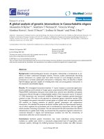
can be plotted in a stitch profile diagram, as illustrated in
Figure 1. The location of a bubble or helix stitch is not
given as a precise coordinate pair (x, y), but rather as a pair
of ds/ss boundaries with fuzzy locations. For each ds/ss

boundary, the range of thermal fluctuations is computed
and given as an interval. A stitch profile indicates a
number of alternative configurations, both optimal and
suboptimal, as illustrated in Figure 1. In contrast, a melt-
ing map would indicate the single configuration at each
What is a stitch profile diagram?Figure 1
What is a stitch profile diagram?. At the top are sketched three alternative DNA conformations at the same temperature.
In the middle diagrams, the sequence location of each helical region (blue) and each bubble or single-stranded region (red) is
represented by a stitch. At the bottom, the three "rows of stitches" are merged into a stitch profile diagram.
0 5 10 15
0 5 10 150 5 10 15
0 5 10 15
Algorithms for Molecular Biology 2008, 3:10 />Page 3 of 20
(page number not for citation purposes)
temperature, in which each basepair is in its most proba-
ble state.
A stitch profile thus provides some features, e.g. bubbles,
that would be of interest in genomic analyses. However,
the previously described algorithm for computing stitch
profiles [29] has time complexity O(N
2
). Genomics stud-
ies often require faster algorithms, both to compute long
sequences and to compute many sequences. In this paper,
therefore, an efficient stitch profile algorithm with time
complexity O(N log N) is described, and the prospects of
computing genomic stitch profiles are discussed. The orig-
inal algorithm [29] is referred to as Algorithm 1, while the
new algorithm is referred to as Algorithm 2.
The reduction in time complexity has been achieved with-

out introducing any approximation or simplification such
as windowing. The usual tradeoff between speed and pre-
cision is therefore not involved here. The output of Algo-
rithm 2 is not of a lower quality, but identical to
Algorithm 1's output. Algorithm 1 was simply inefficient.
However, it was not obvious that this problem has time
complexity O(N log N), which is the same as computing
melting profiles with the Poland-Fixman-Freire algorithm
[32]. It would appear that the stitch profile had greater
complexity, for example, that the search for all bubble
starts and ends would be quadratic. On the other hand,
we know that bubbles may be small compared to the
sequence length. Algorithm 2 detects such circumstances
in an adaptive way, without assuming a maximal bubble
length.
Methods
The proper way of computing DNA conformations, as
well as other macromolecular structures, is to consider a
rugged landscape [33,34]. As an abstract mathematical
function, a landscape applies to widely different complex
systems, for example, fitness landscapes in evolutionary
biology for defining populations and species. The rugged-
ness implies many local maxima and minima on many
levels. In optimization, the task would be to avoid all the
"false" local optima and find the global optimum. That is
not what we want. On the contrary, we would prefer to
include most of them.
A local optimum corresponds to an instantaneous confor-
mation or microstate that is more fit or stable than its
immediate neighbors. However, fluctuations over time

cover a larger area in the landscape around the local opti-
mum, which is defined as a macrostate. A macrostate can
not simply be associated with a local optimum, because it
usually covers many local optima. On the other hand, a
local optimum may be part of different macrostates. Fluc-
tuations are biologically important, as they represent sta-
bility and robustness, rather than noise and uncertainty
[35]. Conformations are properly represented by mac-
rostates, not microstates. We want to characterize the
whole landscape of DNA conformations by a set of mac-
rostates.
More specifically, this article considers certain probability
landscapes, in which the probability peaks are the mac-
rostates. The algorithmic task is to find a set of peaks.
Automatic peak detecting is applied in various kinds of
spectroscopy (NMR), spectrometry (mass-spec), and
image segmentation (e.g. in astronomy), but these algo-
rithms usually do not consider any hierarchical aspects.
Hierarchical peak finding is analogous to hierarchical
clustering, which is widely used in bioinformatics. How-
ever, our approach is closely related to the hierarchical
analyses of energy landscapes and their barriers in studies
of dynamics, metastability, and timescales [36-39]. The
algorithm uses a subroutine for finding hierarchical prob-
ability peaks in one dimension, described in the next sec-
tion.
1D peaks
This section briefly revisits the 1D peak finding method
and the use of a nonstandard pedigree terminology [29].
Here is a generic formulation of the problem: Let p(x) be

some probabilities (possibly marginal) defined for x = 1,
, N . What are the peaks in p(x)? The computational task
is divided into two steps. The first step is to construct a dis-
crete tree of possible peaks, and the second step is to select
peaks by searching the tree.
To simplify the presentation, we assume that p(x
1
) ≠ p(x
2
)
if x
1
≠ x
2
. Let Ψ be the set of x-values, where p(x) has local
minima and maxima. We associate a possible peak with
each element a ∈ Ψ. If a is a local minimum, the peak is
defined as illustrated in Figure 2. The peak location is the
extent on the x-axis, L(a) = [x
start
(a), x
end
(a)], defined as
the largest interval including a in which p(x) ≥ p(a). The
peak width is the size of L(a), p
w
(a) = x
end
(a) - x
start

(a) + 1.
The peak volume is the probability summed over the loca-
tion, p
v
(a) = ∑
x∈L(a)
p(a). The peak's bottom (or mode)
β
a =
arg max
x∈L(a)
p(x) is the x-value where p attains its maxi-
mum. (The term "bottom" originates from the corre-
sponding energy landscape picture, but it is the position
of the peak's top.) The peak height is p
h
(a) = p(
β
a). The
peak's depth is . We also associate a
possible peak with each local maximum a ∈ Ψ, namely
the spike itself: L(a) = [a, a], p
w
(a) = 1,
β
a = a, p
v
(a) = p
h
(a)

= p(a), and D(a) = 0.
Da
pa
pa
() log
()
()
=
10
β
Algorithms for Molecular Biology 2008, 3:10 />Page 4 of 20
(page number not for citation purposes)
While peaks may be high, it is a more defining character-
istic that they are wide. A peak is produced by the fluctua-
tions in x, rather than disturbed by them. For each local
maximum, there are many possible peaks. Therefore, a
peak can not be identified with its bottom. Instead, we use
the elements in Ψ as unique identifiers of peaks. The loca-
tion of a peak is L(a), not the bottom position
β
a, and the
size of a peak is the peak volume, not the peak height.
However, for the second type of peaks (the maxima), the
peak location reduces to the bottom and the peak volume
reduces to the peak height.
The set Ψ of possible peaks is hierarchically ordered. A
binary tree is defined by the set inclusion order on the set
of peak locations. For each pair a, a' ∈ Ψ, either L(a) ⊆
L(a'), or L(a) ⊇ L(a'), or they are disjoint. The branching
corresponds to each local minimum a dividing the peak

into two subpeaks, see Figure 2, just as a barrier or a water-
shed or a saddle point divides two valleys or lakes in a
landscape [36,38,39]. The global minimum is the root
node
ρ
of the tree. The local maxima are the leaf nodes of
the tree. Each a ∈ Ψ has at most three edges, one towards
the root and two away from the root. Each a ≠
ρ
has an
edge towards the root that connects to the successor
σ
a.
Each successor has an increased depth: D(
σ
a) ≥ D(a). And
each local minimum a has two edges away from the root
that connect to two ancestors. The highest peak of the two
ancestors is the father
π
a and the other is the mother
μ
a,
i.e., they are distinguished by p
h
(
π
a) > p
h
(

μ
a). A left-right
distinction between the two is not used. The notation
σ
n
a
means the successor taken n ≥ 0 times, where
σ
0
a = a. Each
a has a set of successors Σ(a) defined as the path from a to
the root: a,
σ
a,
σ
2
a, ,
ρ
. Each a also has a set of ancestors
Δ(a) defined by a' ∈ Δ(a) ⇔ a ∈ Σ(a'). The set Δ(a) is the
subtree that has a as its root node. A bottom is typically
shared by several peaks. For example, a peak has the same
bottom as its father,
β
a =
βπ
a, but not the same as its
mother,
β
a ≠

βμ
a. Each a has a paternal line Π(a), defined
as the set of all nodes that share a's bottom. Π(a) is also
the path including a connected by fathers that ends at
β
a.
The beginning of the path, called the full node
φ
a, is either
a mother or the root. The paternal lines establish a one-to-
one correspondence between the set of maxima (i.e. bot-
toms) and the set of mothers including the root.
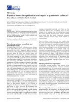
Example of a 1D peakFigure 2
Example of a 1D peak. This peak in p(x) has peak volume (yellow area) p
v
(a) = 1.5 × 10
-72
, while the peak height is p
h
(a) =
2.9 × 10
-73
, which is the maximum probability attained at
β
a = 1209. The peak location L(a) is the extent from x
start
= 1204 to
x
end
= 1216, which corresponds to the local minimum attained at a = 1212. The depth is D(a) = 0.711.

0
p(a)
1e-73
2e-73
p(βa)
1185 1195
x
start
βa a
x
end
1225 1235
p(x)
x (bp)
L(a)
p
h
(a)
p
v
(a)
D(a) = log
10
(p(βa)/p(a))
Algorithms for Molecular Biology 2008, 3:10 />Page 5 of 20
(page number not for citation purposes)
Having established a hierarchy Ψ of possible peaks, the
second step is to select among them. The selection applies
two independent criteria, each controlled by an input
parameter: the maximum depth D

max
and the probability cut-
off p
c
. The first criterion is that a is a 1D peak according to
the following definition.
Definition 1. Let D
max
be the maximum depth of peaks. Then
a ∈ Ψ is a 1D peak if
(i) D(a) <D
max
,
(ii) D(
σ
a) ≥ D
max
or a =
ρ
.
The second criterion is that p
v
(a) ≥ p
c
. The first criterion is
invoked by using the MAXDEEP subroutine [29], which
returns the set P of all 1D peaks. The second criterion is
subsequently invoked by calculating the peak volume of
each a ∈ P and comparing with the probability cutoff.
Bubbles and helical regions

The stitch profile algorithm is separate from the statistical
mechanical DNA melting model. The only interface to the
underlying model is by calling the following probability
functions:
In these equations, 1 is a bound basepair (helix), 0 is a
melted basepair (coil), X is either 0 or 1, and the sequence
positions x and/or y are indicated.
In addition to these, the stitch profile algorithm calls
methods for adding these probabilites (peak volumes)
and for computing upper bounds on such probability
sums. This means that it is easy to change or replace the
underlying model. In this article, the Poland-Scheraga
model with Fixman-Freire loop entropies is used [30], but
in principle, other DNA melting models could be used, or
even models that include secondary structure [40].
This article discusses how to efficiently compute bubble
stitches and helix stitches only. The 5' and 3' tail stitches
are efficiently computed as in Algorithm 1 [29]. Each bub-
ble stitch corresponds to a peak in the bubble probability
function in Eq. (3). And each helix stitch corresponds to a
peak in the helix probability function in Eq. (4). These
two probability functions and their peaks are two dimen-
sional, so the 1D peak finding method does not directly
apply. However, the 1D peak analysis can be performed
for each of the other four probability functions [Eqs. (1),
(2), (5), and (6)]. Using Eq. (1), a binary tree Ψ
x
and a set
of 1D peaks P
x

is computed, and using Eq. (2), a binary
tree Ψ
y
and a set of 1D peaks P
y
is computed. The proba-
bility cutoff is not invoked here. These two tree structures
with their 1D peaks are then further processed, as
described in the following two sections, to obtain the bub-
ble stitches. Likewise, using Eq. (5), a binary tree Ψ
x
and a
set of 1D peaks P
x
is computed, and using Eq. (6), a binary
tree Ψ
y
and a set of 1D peaks P
y
is computed. These are
used similarly to obtain the helix stitches. This division of
labor also indicates an obvious parallelization of the algo-
rithm using two or four processors. Parallelism was not
implemented in this study, however.
2D peaks
The goal of this section is to define 2D peaks and to prove
the key result that some 2D peaks are simply the Cartesian
product of two 1D peaks. But not all 2D peaks have this
property, making it a nontrivial result. This is expressed in
Theorem 2.

Theorem 2 also indicates a convenient way of computing
all 2D peaks, on which Algorithm 2 is directly based. The-
orem 2 shows that Algorithm 2's computation of stitch
profiles is exact, that is, complying strictly with the math-
ematical definition of 2D peaks. The proof is therefore
important for the validation of Algorithm 2. While Theo-
rem 2 is the primary goal, we also prove Theorem 1 which
similarly provides validation of Algorithm 1. But more
importantly, a comparison of the two theorems gives
more insight in both algorithms.
A frame is a pair (a, b) ∈ Ψ
x
× Ψ
y
. A frame also refers to the
corresponding box L(a) × L(b) in the xy-plane. A frame (a,
b) is contained inside another frame (a', b'), if L(a) × L(b) ⊂
L(a') × L(b'), that is, if a' ∈ Σ(a) and b' ∈ Σ(b). The root
frame is (
ρ
x
,
ρ
y
). A frame (a, b) is nonroot if (a, b) ≠ (
ρ
x
,
ρ
y

).
A frame (a, b) is a bottom frame if (a, b) = (
β
a,
β
b) and it is
nonbottom if (a, b) ≠ (
β
a,
β
b). The depth of a frame (a, b) is
pxP
x
right
unzipped
XX() ( ),=−
′
…

10 0 3
(1)
pyP
y
left
unzipped
XX() ( ),=
′
−5001

…

(2)
pxyP
x
y
bubble
bubble
XX XX(,) ( ),= …

…10 01
(3)
pxyP
x
y
helix
helix
XX0 0XX(,) ( ),= …

…11
(4)
pxNP
x
helix
zipped
XX0(, ) ( ),=−
′
…

113
(5)
pyP

y
helix
zipped
XX(, ) ( ).15110=
′
− 

…
(6)
Algorithms for Molecular Biology 2008, 3:10 />Page 6 of 20
(page number not for citation purposes)
D(a, b) = max{D(a), D(b)}. From this definition, we
immediately get
D(a, b) <D
max
⇔ D(a) <D
max
and D(b) <D
max
.(7)
To simplify the presentation, we assume that for all
frames: D(a) ≠ D(b).
Definition 2. The successor of a nonroot frame (a, b) is
A successor of the root frame does not exist.
Having defined the depth and the successor, what is the
depth of a successor?
Proposition 1. For every nonroot (a, b), D(
σ
(a, b)) ≥ D(a,
b).

Proof. For
σ
(a, b) = (
σ
a, b), max{D(
σ
a), D(b)} ≥
max{D(a), D(b)} because D(
σ
a) ≥ D(a). Likewise for
σ
(a,
b) = (a,
σ
b). ᮀ
Definition 3. A frame (a, b) is
σ
-above if
(i) D(
σ
a) > D(b) or a =
ρ
x
,
(ii) D(
σ
b) > D(a) or b =
ρ
y
.

The term "
σ
-above" is a mnemonic for the two inequali-
ties in the definition. The set of all frames that are
σ
-above
is called the frame tree. While Prop. 1 only sets a lower
bound on the depth of a successor, we can write the actual
value for
σ
-above frames:
Proposition 2. If (a, b) is nonroot and
σ
-above, then
Furthermore, D(
σ
(a, b)) = min{D(
σ
a), D(
σ
b)} if both a ≠
ρ
x
and b ≠
ρ
y
.
Proof. If
σ
(a, b) = (

σ
a, b), then a ≠
ρ
x
and max{D(
σ
a),
D(b)} = D(
σ
a) by Def. 3. If, furthermore, b ≠
ρ
y
, then
D(
σ
(a, b)) = D(
σ
a) <D(
σ
b) by Def. 2. Likewise if
σ
(a, b) =
(a,
σ
b). ᮀ
By repeatedly taking the successor, we eventually end up
at the root frame in, say, R steps. Σ(a, b) is the sequence of
successors of (a, b), i.e., the sequence that
begins at (a, b) and ends at the root frame. Alternatively,
Σ(a, b) is defined as the set of successors, i.e., the set of such

sequence elements. What if we want to exclude (a, b) from
Σ(a, b)? That can be written as Σ(
σ
(a, b)).
If (a, b) is not
σ
-above, then its sequence of successors
takes the shortest path to a
σ
-above frame, or put another
way:
Proposition 3. If a' ∈ Σ(a), b' ∈ Σ(b) and (a', b') is
σ
-above,
then (a', b') ∈ Σ(a, b).
Proof. All elements in both Σ(a) and Σ(b) are visited by the
sequence Σ(a, b) on its climb to the root frame. Assume
(a', b') ∉ Σ(a, b). Then either a' is passed before b' is
reached, or viceversa, and we can assume that a' comes
first. In other words, a' ≠
ρ
x
and there is a b" ≠ b' such that
b' ∈ Σ(b") and
σ
(a', b") = (
σ
a', b"). Then D(b') ≥ D(
σ
b").

By Def. 2, we see that D(
σ
b") > D(
σ
a'). (a', b') is
σ
-above,
so by Def. 3, we see that D(
σ
a') > D(b'). We arrive at the
contradiction D(b') > D(b'). ᮀ
Each frame is the successor of at most four frames. If (a, b)
=
σ
(a', b') then (a', b') is either (
π
a, b), (a,
π
b), (
μ
a, b), or
(a,
μ
b). Two of these are defined as ancestors:
Definition 4. The father of a nonbottom frame (a, b) is
The mother of a nonbottom frame (a, b) is
Fathers and mothers of bottom frames do not exist.
Each father or mother can have its own father and mother,
and so on. The set of ancestors Δ(a, b) is the binary subtree
defined recursively by: (1) (a, b) ∈ Δ (a, b). (2) If nonbot-

tom (a', b') ∈ Δ(a, b) then
π
(a', b') ∈ Δ(a, b) and
μ
(a', b')
∈ Δ(a, b).
The next proposition shows that being
σ
-above is propa-
gated by
σ
,
π
, and
μ
:
Proposition 4. Let (a, b) be
σ
-above.
(i) If (a', b') ∈ Σ(a, b) then (a', b') is
σ
-above.
(ii) If (a', b') ∈ Δ(a, b) then (a', b') is
σ
-above.
Proof. (i): First, we show that
σ
(a, b) is
σ
-above: If

σ
(a, b)
= (
σ
a, b), then Def. 2 implies the second condition: D(
σ
b)
σ
σσσρ
σσσ
(,)
(,) () ()
(, ) ( ) ( )
ab
ab ifD b D a orb
abifDa Db
y
=
>=
>

oor a
x
=
⎧
⎨
⎩
ρ
(8)
Dab

D a if ab ab
Dbif ab ab
((,))
() (,)(,)
() (,)(,).
σ
σσ σ
σσ σ
=
=
=
⎧
⎨
⎩


(9)
{(,)}
σ
nR
ab
0
π
π
π
(,)
(,) () ()
(, ) () ()
ab
ab ifDa Db

abifDa Db
=
>
<
⎧
⎨
⎩


(10)
μ
μ
μ
(,)
(,) () ()
(, ) () ().
ab
ab ifDa Db
abifDa Db
=
>
<
⎧
⎨
⎩


(11)
Algorithms for Molecular Biology 2008, 3:10 />Page 7 of 20
(page number not for citation purposes)

> D(
σ
a) or b =
ρ
y
. And (a, b) is
σ
-above which by Def. 3
implies the first condition: D(
σ
2
a) > D(
σ
a) > D(b) or
σ
a =
ρ
x
. Similarly,
σ
(a, b) = (a,
σ
b) is shown to be
σ
-above. The
proof is completed by induction.
(ii): First, we show that
π
(a, b) is
σ

-above: If
π
(a, b) = (
π
a,
b), then Eq. (10) implies the first condition: D(
σπ
a) =
D(a) > D(b) or
π
a =
ρ
x
. And (a, b) is
σ
-above which by Def.
3 implies the second condition: D(
σ
b) > D(a) > D(
π
a) or
b =
ρ
y
. Similarly,
π
(a, b) = (a,
π
b) and
μ

(a, b) are shown to
be
σ
-above. The proof is completed by induction. ᮀ
Successors are the inverse of fathers and/or mothers for
σ
-
above frames only:
Proposition 5. If (a, b) is nonbottom and nonroot, the follow-
ing statements are equivalent:
(i) (a, b) is
σ
-above
(ii)
σπ
(a, b) = (a, b)
(iii)
σμ
(a, b) = (a, b)
(iv)
πσ
(a, b) = (a, b) or
μσ
(a, b) = (a, b)
Proof. (i) ⇔ (ii): If
π
(a, b) = (
π
a, b), then Eq. (10) implies
the first condition that (a, b) is

σ
-above: D(
σ
a) > D(a) >
D(b) or a =
ρ
x
. Then (a, b) is
σ
-above > D(a) =
D(
σπ
a) or b = = (
σπ
a, b) ⇔
σπ
(a, b) =
(a, b). If
π
(a, b) = (a,
π
b), the equivalence is shown simi-
larly.
(i) ⇔ (iii): Replace
π
by
μ
in the above.
(i) ⇔ (iv): If
σ

(a, b) = (
σ
a, b), then Def. 2 implies the sec-
ond condition that (a, b) is
σ
-above: D(
σ
b) > D(
σ
a) >
D(a) or b = ρ
y
. Then (a, b) is
σ
-above D(
σ
a) > D(b)
π
(
σ
a, b) = (
πσ
a, b) or
μ
(
σ
a, b) = (
μσ
a, b) ⇔
π

(
σ
a, b)
= (
πσ
a, b) or µ(
σ
a, b) = (µ
σ
a, b) ⇔
πσ
(a, b) = (a, b) or
µ
σ
(a, b) = (a, b). If
σ
(a, b) = (a,
σ
b), the equivalence is
shown similarly. ᮀ
Accordingly, there is an "inverse" relationship between
the sets of successors and ancestors:
Proposition 6. (a', b') is
σ
-above and (a, b) ∈ Σ(a', b') iff (a,
b) is
σ
-above and (a', b') ∈ Δ(a, b).
Proof. (a, b) ∈ Σ(a', b') implies a path of successors from
(a', b') to (a, b). Prop. 4 shows that all elements in the path

are
σ
-above. Prop. 5(iv) applied to each step in the path
gives an opposite path of ancestors.
Conversely, (a', b') ∈ Σ(a, b) implies a path of ancestors
from (a, b) to (a', b'). Prop. 4 shows that all elements in
the path are
σ
-above. Prop. 5(ii) and (iii) applied to each
step in the path gives an opposite path of successors. ᮀ
It follows from Prop. 6 that the frame tree is equal to the
binary tree Δ(
ρ
x
,
ρ
y
), because (
ρ
x
,
ρ
y
) ∈ Σ(a', b') for any (a',
b'). It has the same pedigree properties as Ψ, such as pater-
nal lines and
βπ
(a, b) =
β
(a, b). So far, we have covered

ground that was already implicit in [29], but augmented
here with proofs. The next concept is new, however,
namely the Cartesian products of 1D peaks.
Definition 5. (a, b) is a grid frame if a and b are 1D peaks.
The set of all grid frames is G = P
x
× P
y
. As Figure 3 shows,
G has a grid-like ordering in the xy-plane. All 1D peaks a
∈ P
x
have disjoint peak locations L(a) = [x
start
(a), x
end
(a)].
They can be indexed by i = 1, 2, 3, according to their
ordering from 5' to 3' on the sequence, such that x
end
(a
i
)
<x
start
(a
i+1
). Likewise, the 1D peaks b ∈ P
y
can be indexed

by j. Then the grid frames form a matrix G with elements
[G]
ij
= (a
i
, b
j
). We use the symbol G for both the set and the
matrix.
Proposition 7. Every grid frame (a, b) is
σ
-above.
Proof. If a ≠
ρ
x
, then D(
σ
a) ≥ D
max
because a is a 1D peak
and D
max
> D(b) because b is a 1D peak (see Def. 1), thus
showing Def. 3(i). Similarly, we show Def. 3(ii). ᮀ
The following two lemmas show that grid frames inherit
some properties from 1D peaks.
Lemma 1. (a, b) is a grid frame iff
(i) (a, b) is
σ
-above,

(ii) D(a, b) <D
max
,
(iii) D(
σ
(a, b)) ≥ D
max
or (a, b) is the root frame.
Proof. If (a, b) is a grid frame, then it is
σ
-above by Prop. 7
and Eq. (7) implies D(a, b) <D
max
. For nonroot (a, b),
D(
σ
(a, b)) equals either D(
σ
a) or D(
σ
b) (Prop. 2), which
is ≥ D
max
because a and b are 1D peaks.
Conversely, Eq. (7) implies D(a) <D
max
. For a =
ρ
x
, a is

then a 1D peak. For a ≠
ρ
x
, Prop. 2 gives D(
σ
a) ≥ D(
σ
(a,
⇔
Def .
()
3
Db
σ
ρσπ
y
Def
=⇔
.
(,)
2
ab
⇔
Def .3
⇔
Def .4
Algorithms for Molecular Biology 2008, 3:10 />Page 8 of 20
(page number not for citation purposes)
b)) ≥ D
max

, so a is a 1D peak. Similarly, b is shown to be a
1D peak. ᮀ
Lemma 2. Let D
max
be the maximum depth of peaks.
(i) For each a with D(a) <D
max
, there is exactly one 1D peak
a' ∈ Σ(a).
(ii) For each (a, b) with D(a, b) <D
max
, there is exactly one grid
frame (a', b') ∈ Σ(a, b).
Proof. (i): The depth increases monotonically in the
sequence Σ(a) of successors (∀n : D(
σ
n
a) ≤ D(
σ
n+1
a)). For
D(
ρ
x
) ≥ D
max
, there is therefore a unique element a' ≠
ρ
x
with D(a') <D

max
and D(
σ
a') ≥ D
max
. For D(
ρ
x
) <D
max
, a' =
ρ
x
is a 1D peak and no other element in Σ(a) can fulfill
Def. 1(ii).
(ii): Eq. (7) gives D(a) <D
max
and D(b) <D
max
. By applying
(i) to a and b, we obtain a unique grid frame (a', b') where
a' ∈ Σ(a) and b' ∈ Σ(a). (a', b') is
σ
-above by Prop. 7, so
(a', b') ∈ Σ(a, b) by Prop. 3. ᮀ
How do we define 2D peaks? A straightforward way
would be to generalize 1D peaks by simply rewriting Def.
1 in the frame tree context. The result would be the grid
frames, as we see by Lemma 1. However, there is more to
the picture than the frame tree, due to a further constraint

to be discussed next, which requires a more elaborate def-
inition of 2D peaks.
In genomic annotations, a region is specified by coordi-
nates x y, where by convention x <y, i.e., x is the 5' end
and y is the 3' end. We adopt the same constraint for our
notation (x, y) of the instantaneous location of a bubble
or helix. In the xy-plane, helices are only defined for (x, y)
above the diagonal line y = x. Bubbles have at least one
melted basepair in between x and y, so they are only
defined for (x, y) above the diagonal line y = x + 1. Accord-
ingly, we require that frames are above the diagonal line,
as defined in the following.
The set G = P
x
× P
y
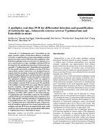
of all grid frames plotted in the xy-planeFigure 3
The set G = P
x
× P
y
of all grid frames plotted in the xy-plane. The grid frames are colored to distinguish those that are
above the diagonal (green), crossing the diagonal (red), and below the diagonal (grey), thus illustrating the subsets G
a
, G
c
and G
b
,
respectively. Frames with side lengths below 20 bp are not shown to unclutter the figure.

0
500
1000
1500
2000
2500
3000
3500
4000
4500
0 500 1000 1500 2000 2500 3000 3500 4000 4500
y (bp)
x (bp)
Algorithms for Molecular Biology 2008, 3:10 />Page 9 of 20
(page number not for citation purposes)
Definition 6. A frame (a, b) is above the diagonal if
x
end
(a) + 1 <y
start
(b) for bubbles, (12a)
x
end
(a) <y
start
(b) for helices. (12b)
A frame (a, b) is below the diagonal if
x
start
(a) + 1 ≥ y

end
(b) for bubbles, (13a)
x
start
(a) ≥ y
end
(b) for helices. (13b)
A frame (a, b) is crossing the diagonal if it is neither above
the diagonal nor below the diagonal.
Note: A frame that is crossing the diagonal contains at
least one point (x, y) above the diagonal line, while a
frame that is below the diagonal contains no points above
the diagonal line, but its upper left corner may be on the
diagonal line. Figure 3 illustrates frames that are above,
crossing and below the diagonal.
The requirement that a frame is above the diagonal puts a
constraint on its size. This is embodied in the next con-
cept.
Definition 7. The root frame is a fractal frame if it is above
the diagonal. A nonroot frame (a, b) is a fractal frame if
(i) (a, b) is above the diagonal,
(ii)
σ
(a, b) is crossing the diagonal,
(iii) (a, b) is
σ
-above.
The set of all fractal frames is denoted F. As Figure 4
shows, fractal frames tend to be smaller the closer they are
to the diagonal, thus resembling a fractal. For a typical

fractal frame, the fluctuations in x and y are comparable in
size to the length y - x of the bubble or helix itself. Indeed,
The set F of all fractal frames plotted in the xy-planeFigure 4
The set F of all fractal frames plotted in the xy-plane. The fractal frames (a, b) ∈ F are colored to distinguish those with
depths D(a, b) ≥ D
max
(grey) and D(a, b) <D
max
(blue), thus illustrating the subsets F
d
and F
s
, respectively. Frames with side
lengths below 20 bp are not shown to unclutter the figure.
0
500
1000
1500
2000
2500
3000
3500
4000
4500
0 500 1000 1500 2000 2500 3000 3500 4000 4500
y (bp)
x (bp)
the diagonal
fractal frames (deep)
fractal frames (shallow)

Algorithms for Molecular Biology 2008, 3:10 />Page 10 of 20
(page number not for citation purposes)
the two peak locations L(a) and L(b) are as wide as possi-
ble, while not overlapping each other (because the succes-
sor is crossing the diagonal). In contrast, the fluctuations
for grid frames are relatively small on average and inde-
pendent of the bubble or helix length.
Lemma 3. For each
σ
-above and above the diagonal (a, b),
there is exactly one fractal frame (a', b') ∈ Σ(a, b).
Proof. Let (a', b') =
σ
n
(a, b), where n is the largest number
for which
σ
n
(a, b) is above the diagonal. (a', b') is
σ
-above
by Prop. 4. For all m > n, frames
σ
m
(a, b) (if they exist) are
not above the diagonal, nor below the diagonal because
they contain (a, b), hence they are crossing the diagonal.
Therefore (a', b') is a fractal frame. For all m <n, frames
σ
m

(a, b) (if they exist) are above the diagonal, because
they are contained in (a', b'). Therefore (a', b') is the only
fractal frame in Σ(a, b). ᮀ
Lemma 3 is similar to Lemma 2. By Prop. 6, we can
express both lemmas in terms of ancestors Δ instead of
successors Σ. The lemmas then say that certain kinds of
frames are organized as forests. A forest is a set of disjoint
trees. The sets F and G generate two forests: ∪
(a, b) ∈ G
Δ(a,
b) consists of the subtrees having grid frames as root
nodes. ∪
(a,b) ∈ F
Δ(a, b) consists of the subtrees having frac-
tal frames as root nodes. By these forests, we generate
from G the set of all
σ
-above frames with D(a, b) <D
max
,
and we generate from F the set of all
σ
-above frames above
the diagonal.
All the necessary concepts are now in place for the defini-
tion of 2D peaks. We will not repeat the "derivation" of
2D peaks given in [29], but just recall that 2D peaks are
defined with a purpose: They must capture the extent of
the actual peaks in the probability functions p
bubble

(x, y)
and p
helix
(x, y). And they must have an interpretation in
terms of fluctuations on a given timescale. The following
definition is equivalent to the formulation in [29].
Definition 8. Let D
max
be the maximum depth of peaks. A
frame (a, b) is a 2D peak if
(i) (a, b) is above the diagonal,
(ii) (a, b) is
σ
-above,
(iii) D(a, b) <D
max
,
(iv) D(
σ
(a, b)) ≥ D
max
or (a, b) is a fractal frame.
Note: the or in the definition is not an exclusive or. A 2D
peak (a, b) can both be a fractal frame and have D(
σ
(a, b))
≥ D
max
. The set of all 2D peaks is denoted P and is illus-
trated in Figure 5.

Comparing Def. 8 and Lemma 1, we see that the differ-
ence between 2D peaks and grid frames is due to the diag-
onal constraint: First, the requirement that 2D peaks are
above the diagonal, and second, the possible exemption
from the second inequality, which for grid frames is being
the root frame, while for 2D peaks it is being a fractal
frame. Unlike grid frames, 2D peaks can capture events
close to the diagonal by adapting their size.
Computing the 2D peaks is at the core of the stitch profile
methodology. The following two theorems provide char-
acterizations of 2D peaks that may be translated into com-
puter programs.
Theorem 1. We divide 2D peaks into two types, being fractal
frames or not, that can be distinctly characterized as follows.
(i) (a, b) is a 2D peak and a fractal frame iff (a, b) is a fractal
frame and D(a, b) <D
max
.
(ii) (a, b) is a 2D peak and not a fractal frame iff (a, b) is a
grid frame and there is a fractal frame (a', b') with D(a', b') ≥
D
max
, such that (a', b') ∈ Σ(a, b).
Proof. (i): Immediate by Defs. 7 and 8.
(ii): If a 2D peak (a, b) is not a fractal frame, then D(
σ
(a,
b)) ≥ D
max
by Def. 8, so (a, b) is a grid frame by Lemma 1.

Applying Lemma 3, there is a fractal frame (a', b') ∈ Σ(a,
b). (a, b) ≠ (a', b') because one is a fractal frame, the other
is not, so (a', b') ∈ Σ(
σ
(a, b)), which by Prop. 1 implies
D(a', b') ≥ D
max
.
Conversely, (a, b) is above the diagonal because it is con-
tained in a fractal frame. (a, b) ≠ (a', b') because D(a, b)
<D
max
and D(a', b') ≥ D
max
, implying that (a, b) is not a
fractal frame (uniqueness by Lemma 3) and not the root
frame. The other requirements for a 2D peak are estab-
lished by Lemma 1. ᮀ
Theorem 1 characterizes all 2D peaks by their relationship
to fractal frames. This is applied in Algorithm 1, that
derives all 2D peaks from fractal frames. However, the
next theorem shows that some 2D peaks can be character-
ized without referring to fractal frames.
Theorem 2. A nonroot 2D peak has a successor, the depth of
which is either greater or less than D
max
. We thus divide 2D
peaks into two types, that can be distinctly characterized as fol-
lows. Let (a, b) be nonroot. Then
(i) (a, b) is a 2D peak and D(

σ
(a, b)) ≥ D
max
iff (a, b) is a grid
frame that is above the diagonal.
Algorithms for Molecular Biology 2008, 3:10 />Page 11 of 20
(page number not for citation purposes)
(ii) (a, b) is a 2D peak and D(
σ
(a, b)) <D
max
iff (a, b) is a
fractal frame and there is a grid frame (a', b') that is crossing
the diagonal, such that (a', b') ∈ Σ(a, b).
Proof. (i): Immediate by Def. 8 and Lemma 1.
(ii): If a 2D peak (a, b) has D(
σ
(a, b)) <D
max
, then (a, b) is
a fractal frame by Def. 8. Applying Lemma 2 to
σ
(a, b),
there is a grid frame (a', b') ∈ Σ(
σ
(a, b)) ⊂ Σ(a, b). Frame
(a', b') is crossing the diagonal because it contains
σ
(a, b),
which is crossing the diagonal because (a, b) is a fractal

frame.
Conversely, (a, b) ≠ (a', b') because (a, b) is above the diag-
onal (a fractal frame) and (a', b') is crossing the diagonal,
and hence (a', b') ∈ Σ(
σ
(a, b)). Since (a', b') is a grid frame,
Lemma 1 gives D(a', b') <D
max
, which by Prop. 1 implies
D(a, b) ≤ D(
σ
(a, b)) <D
max
, and we conclude that (a, b) is
a 2D peak. ᮀ
Note: Theorem 2 does not consider the root frame. How-
ever, if the root frame is a 2D peak, then it is of the first
type: a grid frame that is above the diagonal.
It follows from Theorems 1 and 2 that a 2D peak is either
a grid frame, a fractal frame, or both. The set of 2D peaks
P can therefore be divided into three disjoint sets defined
as follows. P
F
are the 2D peaks that are fractal frames only,
not grid frames. P
FG
are the 2D peaks that are both fractal
frames and grid frames. P
G
are the 2D peaks that are grid

frames only, not fractal frames. Let G
a
, G
b
and G
c
be the
sets of grid frames that are above, below and crossing the
diagonal, respectively. Let F
d
and F
s
be the sets of fractal
frames that are deep (D(a, b) ≥ D
max
) and shallow (D(a, b)
<D
max
), respectively. In Figs. 3, 4, 5, all these subsets are
illustrated with different colors. The following corollary
summarizes the relationships between grid frames, fractal
frames and 2D peaks:
Corollary 1. The set of 2D peaks is P = F
s
∪ G
a
. The intersec-
tion between the grid and the fractal is P
FG
= F

s
∩ G
a
= F ∩ G.
The set P of all 2D peaks plotted in the xy-planeFigure 5
The set P of all 2D peaks plotted in the xy-plane. The 2D peak frames are colored to distinguish those that are fractal
frames (blue), fractal frames and grid frames (black), or grid frames (green), thus illustrating the subsets P
F
, P
FG
and P
G
, respec-
tively. Frames with side lengths below 20 bp are not shown to unclutter the figure.
0
500
1000
1500
2000
2500
3000
3500
4000
4500
0 500 1000 1500 2000 2500 3000 3500 4000 4500
y (bp)
x (bp)
the diagonal
2D peak frames (grid and fractal)
2D peak frames (grid only)

2D peak frames (fractal only)
Algorithms for Molecular Biology 2008, 3:10 />Page 12 of 20
(page number not for citation purposes)
Furthermore, the 2D peaks can be obtained by the following
two expressions, in which all set unions are between disjoint
sets:
Proof. P = P
F
∪ P
FG
∪ P
G
. Theorem 1 states that P
F
∪ P
FG
=
F
s
and that
Here, Δ(a', b') is brought into play by Prop. 6. Theorem 2
states that P
FG
∪ P
G
= G
a
(the root frame would go here)
and that
Eqs. (14a) and (14b) outline how the set of 2D peaks is

built up computationally by Algorithm 1 and 2, respec-
tively. Writing the expressions side by side shows the par-
allels: Algorithm 1 takes some fractal frames and then it
adds some grid frames that are contained inside fractal
frames. Algorithm 2 takes some grid frames and then it
adds some fractal frames that are contained inside grid
frames. In both cases, the additional part is the more com-
plicated part, as it requires searching some forests. The
two Algorithms are algorithmically equivalent in terms of
output, but the transformation in Eq. (14) from F -based
to G-based facilitates a reduction in execution time, as
described in the next section.
The fast and exact algorithm
Algorithm 2 owes its speed to two important ingredients:
One is the grid frame matrix G associated to the parameter
D
max
. The other is an upper bound associated to the
parameter p
c
.
To compute all bubble stitches of the stitch profile, the
algorithm must find those 2D peaks (a, b) in the bubble
context that have a peak volume
that is greater or equal to the probability cutoff p
c
. Accord-
ing to Eq. (14b), one can write an algorithm for obtaining
all 2D peaks using two nested loops that goes through all
matrix elements (a

i
, b
j
) of the grid frame matrix G: If (a
i
,
b
j
) is above the diagonal, it is a 2D peak. If (a
i
, b
j
) is cross-
ing the diagonal, a subroutine computes the set F ∩ Δ(a
i
,
b
j
). If (a
i
, b
j
) is below the diagonal, it is skipped. By piping
the resulting frames through a probability cutoff filter, we
obtain the bubble stitches.
The matrix G is not stored in memory, only the two arrays
P
x
and P
y

that provide each a
i
and b
j
. Matrix elements (a
i
,
b
j
) being above, crossing or below the diagonal refers to
the diagonal line in the xy-plane, never the diagonal of the
matrix. For each row and column of the matrix there may
be zero, one, or more matrix elements that are crossing the
diagonal, as can be seen in Figure 3.
More specifically, let G be of order m × n and let the outer
loop be over j = n to 1 and the inner loop over i = m to 1.
The iteration thus begins at the upper right corner of Fig-
ure 3 and steps along the y-axis in the outer loop and the
x-axis in the inner loop. However, we do not have to start
at i = m for each j. If (a
i
, b
j
) is below the diagonal, then (a
i
,
b
k
) is below the diagonal for all k < j. Therefore, we can
jump directly to the i that corresponds to the first grid

frame that was not below the diagonal at the previous j. In
this way, most of the grid frames that are below the diag-
onal are ignored by the algorithm. While this is a trivial
programming trick, we shall now see a less trivial trick,
that ignores most of the grid frames that are above the
diagonal.
Recall [30] that the bubble probability is
The loop entropy factor Ω(y - x) is a monotonically
decreasing function. Its largest value in a frame (a, b) is
therefore in the lower right corner, i.e. Ω
max
= Ω(y
start
(b) -
x
end
(a)). Then
and the bubble peak volume has an upper bound that fac-
torizes. Using the 1D peak volumes
we can write the upper bound as
PF G ab
s
ab F
d
=∩
′′
′′
∈
Δ(,),
(,)

∪
(14a)
=∩
′′
′′
∈
GFab
a
ab G
c
Δ(,).
(,)
∪
(14b)
PGab
G
ab F
d
=∩
′′
′′
∈
Δ(,).
(,)
∪
PFab
F
ab G
c
=∩

′′
′′
∈
Δ(,).
(,)
∪

pab p xy
yLbxLa
v bubble
(,) (,)
()()
=
∈∈
∑∑
(15)
pab
ZxyxZy
Z
bubble
XX
(,)
() ( ) ()
.=
−
10 01
Ω
(16)
pab
Z

Zx Zy
xLa yLb
vXX
(,)
max
() ()
() ()
≤
⎛
⎝
⎜
⎜
⎞
⎠
⎟
⎟
⎛
⎝
⎜
⎜
⎞
⎠
⎟
⎟
∈∈
∑∑
Ω
10 01
pa Z x Z
xLa

vX
() ()/ ,
()
=
∈
∑
10
(17a)
pb Z y Z
yLb
vX
() ()/ ,
()
=
∈
∑
01
(17b)
Algorithms for Molecular Biology 2008, 3:10 />Page 13 of 20
(page number not for citation purposes)
If a grid frame (a
i
, b
j
) has an upper bound below the cut-
off, (a
i
, b
j
) <p

c
, then also (a
k
, b
j
) <p
c
for all k < i for
which p
v
(a
k
) ≤ p
v
(a
i
), because the loop entropy factor is
decreasing. In that case, their peak volumes are also below
the cutoff, of course, and the algorithm can reject all these
frames. We implement this observation by calculating in
advance the next bigger goat nbg(i) defined by
(i) p
v
(a
k
) ≤ p
v
(a
i
) for nbg(i) <k < i

(ii) p
v
(a
nbg(i)
) > p
v
(a
i
)
The nbg(i) is calculated as follows: A loop over i = 1 to m
compares each p
v
(a
i
) successively to p
v
(a
i-1
), p
v
(a
nbg(i-1)
), p
v
(a
nbg(nbg(i-1))
), until a bigger one is found or the list ends.
For grid frames (a
i
, b

j
) that are above the diagonal, the
algorithm first checks if (a
i
, b
j
) <p
c
, in which case it
jumps directly to (a
nbg(i)
, b
j
). The nbg(i) may be unde-
fined, if there are no bigger p
v
(a
k
), in which case the inner
loop is done and the outer loop proceeds to the next j. On
the other hand, if (a
i
, b
j
) ≥ p
c
, then the peak volume has
to be calculated and checked. Although grid frames may
be skipped without having calculated neither their peak
volumes nor their upper bounds, the criterion for rejec-

tion is exact. There are no false negatives (or positives).
For each grid frame (a
i
, b
j
) that is crossing the diagonal,
the algorithm calculates a set of 2D peaks, F ∩ Δ(a
i
, b
j
),
and checks the peak volume of each. This set consists of all
fractal frames that are contained inside (a
i
, b
j
). A mental
picture is that (a
i
, b
j
) must be broken into fractal frames
(fractured) to avoid crossing the diagonal. The algorithm
searches the subtree Δ(a
i
, b
j
) top-down (breadth-first)
with a recursive subroutine. A given input frame (a, b) is
split into its father frame

π
(a, b) and mother frame
μ
(a, b).
Each in turn is then checked as follows: If it is crossing the
diagonal, it is further split by giving it recursively as input
to the subroutine. If instead it is above the diagonal, it is
a fractal frame. With (a
i
, b
j
) as input, the subroutine finds
F ∩ Δ(a
i
, b
j
). (If instead the input is the root frame (
ρ
x
,
ρ
y
),
the subroutine will find all fractal frames F . This was
applied in Algorithm 1.)
Figure 6 shows the resulting search process, by plotting
only frames that are processed by the algorithm, while the
ignored grid frames are blank. Comparing with Figure 3,
we see that the blank areas correspond to the great bulk of
grid frames both above and below the diagonal, leaving

just an irregular band of frames along the diagonal to be
searched. This is a nice geometric illustration of the reduc-
tion from O(N
2
) to O(N log N) in execution time. Figure
6 also shows that some bubble stitches are fractal frames
contained inside grid frames that are crossing the diago-
nal.
The peak volumes p
v
(a, b) of some frames must be calcu-
lated. Algorithm 2 spends a considerable fraction of its
time on doing these summations. The summation over a
bubble frame can be done faster if the frame is big
enough, by exploiting the Fixman-Freire approximation à
la Yeramian [32,41]. This does not improve the time com-
plexity, but significantly reduces the total execution time
by some factor.
To compute all helix stitches of the stitch profile, the algo-
rithm follows exactly the same procedure as described
above, but in the helix context. Eq. (14b) and the analysis
in the previous section applies equally well to the bubble
and the helix contexts. The various quantities are, of
course, replaced by their helix counterparts. For example,
the appropriate diagonal line is applied (Def 6). The main
difference is the upper bound on helix peak volume. Since
x and y decouples in the helix probability [29],
we can simply use the peak volume as its own upper
bound:
The Ξ (x, y) factor [29] is the counterpart of Ω(y - x), but

an explicit consideration of its monotonicity is not neces-
sary here, because it is absorbed in the above quantities. A
next bigger goat is then calculated and applied in the same
way as for bubbles.
Results and Discussion
Time complexity
By inspection of Algorithm 2, we observe that it visits at
least O(N) and at most O(N
2
) matrix elements of G. Fur-
thermore, it performs sorting, which is known to scale as
O(N log N). The time complexity is therefore between
O(N log N) and O(N
2
). The execution time depends on
the fraction of ignored grid frames above the diagonal,
which depends on the specific sequence, temperature, and
other input parameters. A theoretical analysis of these
dependencies is complicated.

pab y b x aZpapb
vstartendvv
(,) ( () ()) () ().=−Ω
(18)

p
v

p
v


p
v

p
v
pxy
pxNp y
pN
helix
helix helix
helix
(,)
(, ) (,)
(, )
,=
1
1
(19)

pab pab
papb
pN
vv
vv
helix
(,) (,)
() ()
(, )
.==

1
(20)
Algorithms for Molecular Biology 2008, 3:10 />Page 14 of 20
(page number not for citation purposes)
Empirical testing of the execution times were done
instead, using a test set of 14 biological sequences with
lengths selected to be evenly spread on a log scale span-
ning three decades. A minimum length of 1000 bp was
required. Most of the test sequences are genomic
sequences, so as to represent the typical usage of the algo-
rithm. The sequence lengths and accession numbers are:
• 1168 bp [GenBank:BC108918
]
• 1986 bp [GenBank:BC126294
]
• 4781 bp [GenBank:BC039060
]
• 7904 bp [GenBank:NC_001526
]
• 16571 bp [GenBank:NC_001807
]
• 36001 bp [GenBank:AC_000017
]
• 48502 bp [GenBank:NC_001416
]
• 85779 bp [GenBank:NC_001224
]
• 168903 bp [GenBank:NC_000866
]
• 235645 bp [GenBank:NC_006273

]
• 412348 bp [GenBank:AE001825
]
• 816394 bp [GenBank:NC_000912
]
• 1138011 bp [GenBank:AE000520
]
• 2030921 bp [GenBank:NC_004350
]
The algorithms were written in Perl and run on a Pentium
4, 2.4 GHz, 512 KB cache, 1 GB memory, PC with Linux
(CentOS). In Figure 7, the speeds of Algorithms 1 and 2
The footprints of Algorithm 2 plotted in the xy-planeFigure 6
The footprints of Algorithm 2 plotted in the xy-plane. These are frames that are visited by Algorithm 2 during its search
for the bubble stitches (filled yellow). The frames are located in a band along the diagonal, suggesting that the search space is
proportional to sequence length. Grid frames below the diagonal (grey) are skipped. Grid frames crossing the diagonal (red)
are broken into fractal frames (blue). The bubble stitches (filled yellow) are those grid frames above the diagonal (green) and
fractal frames (blue) that have p
v
(a, b) ≥ p
c
. Frames with side lengths below 20 bp are not shown to unclutter the figure.
0
500
1000
1500
2000
2500
3000
3500

4000
4500
0 500 1000 1500 2000 2500 3000 3500 4000 4500
y (bp)
x (bp)
the diagonal
bubble stitches
grid frames above the diagonal
grid frames below the diagonal
fractal frames
grid frames crossing the diagonal
Algorithms for Molecular Biology 2008, 3:10 />Page 15 of 20
(page number not for citation purposes)
are compared. Algorithm 2 is orders of magnitude faster
than Algorithm 1 for sequences longer than 100 kbp.
While all the 14 sequences were computed by Algorithm
2, the three longest sequences were aborted by Algorithm
1, because of too long execution times. To ensure that the
computational tasks were comparable, all sequences were
computed at their melting temperatures T
m
, rather than
one temperature for all, such that all sequences had the
same fractions of helical regions and bubbles. For both
algorithms, straight lines were fitted to the data in the log-
log plot. For Algorithm 2, however, the longest sequence
(2 Mbp) is considered an outlier and thus excluded from
the fit. This sequence's execution time was overly
increased, because the required memory exceeded the
available 1 gigabyte RAM. For Algorithm 1, the slope of

the fit is 1.97955 ± 0.02923, suggesting that it has time
complexity O(N
2
). For Algorithm 2, the slope of the fit is
0.99953 ± 0.02016. This is interpreted as the time com-
plexity O(N log N), but with the logarithmic component
being too weak to distinguish O(N log N) from O(N).
The execution time of Algorithm 2 is just as much a prop-
erty of the underlying energy landscape depending on the
input, as it is a property of the algorithm. Could it be that
other input parameters and/or sequences than was used in
Figure 7 – say, away from the melting points – would
exhibit the time complexity O(N
2
)? Figure 8 shows the
speed of Algorithm 2 over the whole melting range of
temperatures. Each sequence in the test set was computed
at temperatures corresponding to the helicity values:
0.9995, 0.999, 0.995, 0.99, 0.95, 0.9, 0.8, 0.7, , 0.2, 0.1,
0.05, 0.01, 0.005, 0.001, and 0.0005. This helicity range
approximately corresponds to the temperature range T
m
±
10°C and it covers most of the melting transitions.
Although the curves for the individual helicity values may
not be easily distinguished in Figure 8, it appears that all
curves have similar slopes and that they are close to each
other, i.e., the variation in execution time is below 50%.
This indicates that the helicity (or temperature) value has
only a small influence on the total execution time. The

time complexity O(N log N) seems to be robust.
However, a stronger temperature dependence is revealed
when considering the computations of bubble stitches
and helix stitches separately. Two independent subrou-
tines of Algorithm 2 compute the bubble stitches and the
helix stitches, both following the procedure outlined in
the previous section. The rest of Algorithm 2's computa-
tion, including the initial computation of at least four par-
tition function arrays [30], is called the overhead.
Correspondingly, the total execution time t
total
is the sum
of the bubble execution time t
bubble
, the helix execution
time t
helix
, and the overhead execution time t
overhead
. By
simply switching off the bubble subroutine (i.e. t
bubble
= 0)
and measuring the total execution time, we obtain t
helix
+
t
overhead
. Likewise, by switching off the helix subroutine,
Algorithm 1 is quadratic and Algorithm 2 is linearFigure 7

Algorithm 1 is quadratic and Algorithm 2 is linear. The log-log plot shows the execution time versus sequence length of
Algorithm 1 (red) and Algorithm 2 (blue). The straight lines are fits to the data points with slopes 1.97955 ± 0.02923 (red) and
0.99953 ± 0.02016 (blue).
1
10
100
1000
10000
100000
1e+06
1000 10000 100000 1e+06 1e+07
Execution time (seconds)
Sequence length N (bp)
Algorithm 1
Algorithm 2
Algorithms for Molecular Biology 2008, 3:10 />Page 16 of 20
(page number not for citation purposes)
we measure t
bubble
+ t
overhead
. In the following, we refer to
t
bubble
+ t
overhead
as the bubble time and t
helix
+ t
overhead

as the
helix time. As an example, Figure 9 shows the results for
the 16571 bp [GenBank:NC_001807
]. The bubble and
helix times are divided by sequence length and plotted as
a function of temperature. Both of them have clearly a
strong temperature dependence. The melting curve is also
plotted in Figure 9, indicating that most of the melting
occurs in the temperature range 80–85°C. Plots like Fig-
ure 9 were made for each sequence in the test set, but the
average behavior is more interesting. To average times of
the order O(N) over sequences of different lengths, one
should divide them by sequence length as in Figure 9.
However, to plot as a function of temperature would not
be meaningful, because the sequences have different T
m
's
and different melting ranges. On the horizontal axis,
instead, we use a normalized temperature,
defined such that the melting curve becomes a sigmoid:
For each
τ
-value (or equivalently for each Θ-value), the
bubble times and helix times divided by sequence length
averaged over all sequences are plotted in Figure 10. The
curves have a similar temperature dependence as in Figure
9. The helix time decreases monotonically (except for a
shoulder), while the bubble time increases monotonically
(except for a shoulder). Both of them have an about four-
fold difference between their maximum and minimum.

Qualitatively, the curves are kind of mirror symmetric, but
the helix time is generally greater than the bubble time,
the two curves cross each other at Θ = 0.12. It seems that
adding the two curves would give a more or less horizon-
tal curve, i.e., the total execution time has much less tem-
perature dependence.
We may understand this interchange between bubble
time and helix time in terms of the melting process. If we
assume that the bubble time is proportional to the area of
the footprint in Figure 6, and that this is proportional to
the average length of potential bubbles at that tempera-
τ
=
−
log( ),
1 Θ
Θ
(21)
Θ=
+
1
1 exp( )
.
τ
(22)
Algorithm 2 is fast at all temperaturesFigure 8
Algorithm 2 is fast at all temperatures. The total execution times are plotted versus sequence length for each of the
listed helicity values.
1
10

100
1000
10000
1000 10000 100000 1e+06 1e+07
Execution time (seconds)
Sequence length N (bp)
Algorithm 2
Helicities:
0.9995
0.9990
0.9950
0.9900
0.9500
0.9000
0.8000
0.7000
0.6000
0.5000
0.4000
0.3000
0.2000
0.1000
0.0500
0.0100
0.0050
0.0010
0.0005
Algorithms for Molecular Biology 2008, 3:10 />Page 17 of 20
(page number not for citation purposes)
ture, then we would expect the bubble time to increase

with temperature, because bubbles grow as DNA melts.
Likewise, we would expect the helix time to decrease with
temperature, because helical regions diminish as DNA
melts.
In this article, Blake & Delcourt's parameter set [42] as
modified by Blossey & Carlon [43] was used with [Na
+
] =
0.075 M. Parameters for the loop entropy approximation
was obtained with our online tool [31,44]. The maximum
depth and probability cutoff parameters were D
max
= 5
and p
c
= 0.01 in Figs. 3, 4, 5, 6, D
max
= 3 and p
c
= 0.02 in
Figure 7, and D
max
= 3 and p
c
= 0.0001 in Figs. 8, 9, 10. The
sequence [GenBank:BC039060
] was used for producing
Figs. 2, 3, 4, 5, 6. A systematic test of how the execution
time depends on D
max

and p
c
has not been performed.
Discussion
For an algorithm to be called efficient, it should solve the
task at hand with optimal time complexity. It should not
introduce approximations, that would just amount to a
reformulation of a simpler, but different task. In this
study, the task is to compute a stitch profile based on the
Poland-Scheraga model with Fixman-Freire loop entro-
pies. With this model, the time complexity must be at
least O(N log N). Indeed, this is achieved by Algorithm 2
under a wide range of conditions. Algorithm 2 does not
acquire a speedup by any windowing approximation, by
which the sequence would first be split into smaller inde-
pendent sequences. Neither does it rely on limiting the
problem to a maximal bubble length. Therefore, Algo-
rithm 2 is efficient. In computational RNA and protein
studies, a maximal loop size is sometimes imposed as a
heuristic for reducing time complexity by one order. Sim-
ilarly, a maximal DNA bubble size of 50 bp has been
reported in computations of low temperature bubble
probabilities in the Peyrard-Bishop-Dauxois model [14].
In contrast, Algorithm 2 can find bubbles of whatever size
at any temperature. In the 48502 bp [Gen-
Bank:NC_001416
], for example, bubbles and helical
regions may be up to around 20000 bp long [45].
Although Algorithm 2 has no explicit notion of a maximal
bubble length, it may implicitly detect length limitations

for both bubbles and helical regions by the absence of the
"next bigger goat". In this way, Algorithm 2 can adapt to
the input sequence. This adaptation is evident in Figure
10, where the bubble execution time grows as bubbles get
bigger at higher temperatures. Conversely, the helix execu-
tion time decreases as the helical regions gradually melt
away.
However, the time complexity was not proven to be O(N
log N) under all conditions. It is still an open question
whether there is a transition to time complexity O(N
2
) in
Bubble and helix execution times versus temperatureFigure 9
Bubble and helix execution times versus temperature. For the sequence [GenBank:NC_001807
], the bubble time (red)
and helix time (green) divided by sequence length (16571 bp) is plotted versus T. The melting curve (blue) shows the helicity Θ
(on the right vertical axis) as a function of T, indicating the melting midpoint: Θ = 0.5 at T
m
= 83.7°C.
0
0.0005
0.001
0.0015
0.002
75 80 85 90 95
0
0.1
0.2
0.3
0.4

0.5
0.6
0.7
0.8
0.9
1
Execution time per bp (seconds)
Helicity
T (
o
C)
melting curve
bubbles
helices
Algorithms for Molecular Biology 2008, 3:10 />Page 18 of 20
(page number not for citation purposes)
some peripheral regions of the input parameter space. But
based on results so far, a fast computation would be
expected in most situations.
How fast is Algorithm 2? Figures 7 and 8 show that the
Perl implementation runs on an old desktop PC at the
speed of roughly 1000 basepairs per second. With today's
computers, assuming twice that speed and enough mem-
ory, the E. coli genome would take 39 minutes, the yeast
genome would take 1.7 hours, and the largest human
chromosome would take 35 hours. In some types of low
temperature melting studies, the features of interest are
the bubbles rather than the helical regions. In such appli-
cations, switching off the computation of helix stitches
can speed up the algorithm several times. As Figure 10

indicates, the helix time is about twice the bubble time at
helicity equal to 0.95, that is, the speedup would be about
threefold. The largest human chromosome would be
done in ten hours. On a computer cluster, the human
genome could be computed in a day. Such bubbles could
then be compared to TFBS, TSS, replication origins, viral
integration sites, etc.
The required memory grows with sequence length and for
sequences longer than 2 Mbp, more than 1 GB was
needed. The memory usage has not been tested further
and the space complexity has not been discussed in this
article. Some memory optimization of the Perl implemen-
tation must be done before such test can reflect the space
complexity. While the algorithm is efficient in terms of
time complexity, the code has room for optimization of
both speed and memory usage. However, the space com-
plexity is believed to be O(N), which means that the algo-
rithm would eventually become out of memory for long
enough sequences. A standard solution is to introduce
efficient use of disk space instead, which could reduce the
memory usage to O(1), without increasing the time com-
plexity.
The fast algorithm presented in this paper relies on a fac-
torization of certain upper bounds, which in turn relies on
a factorization of partition functions in the Poland-Scher-
aga model, see Eq. (16). In general, it seems that a factor-
ization of partition functions is essential for solving DNA
and RNA models in polynomial time. However, some
DNA melting models that explicitly consider supercoiling
do not allow such a factorization [46]. For the purpose of

genomic applications, supercoiling and a number of other
in vivo interactions and constraints in the cell should ide-
ally be accounted for in future DNA model development
[1,15]. Such modelling requires quantitative knowledge
yet to be obtained experimentally. When such data
Sequence-averaged bubble and helix execution timesFigure 10
Sequence-averaged bubble and helix execution times. The bubble time per basepair (red) and helix time per basepair
(green) averaged over all sequences are plotted versus the normalized temperature
τ
for each of the helicity values listed in Fig-
ure 8. The melting curve (blue) shows the helicity Θ (on the right vertical axis) as a function of
τ
, indicating the melting mid-
point: Θ = 0.5 at
τ
= 0.
0
0.0005
0.001
0.0015
0.002
-10 -5 0 5 10
0
0.1
0.2
0.3
0.4
0.5
0.6
0.7

0.8
0.9
1
Execution time per bp (seconds)
Helicity
normalized temperature τ
melting curve
bubbles
helices
Algorithms for Molecular Biology 2008, 3:10 />Page 19 of 20
(page number not for citation purposes)
becomes available, a main challenge will be to develop
models and algorithms that can be solved in time O(N log
N), which is necessary for many genomic applications.
Conclusion
The fast algorithm described in this article enables the
computation of stitch profiles of genomic sequences.
Melting features of interest, such as bubbles, helical
regions, and their boundaries, are computed directly,
rather than relying on visualization or educated guesses.
The algorithm is exact. It does not achieve its speed by
approximations, such as windowing or maximal bubble
sizes. Genomewide comparisons of bubbles with TSS, rep-
lication origins, viral integration sites, etc., are proposed.
The algorithm is available in Perl code from the author.
Online computation of stitch profiles is available on our
web server, which has recently been upgraded to run Algo-
rithm 2 [31,44].
Competing interests
The author declares that they have no competing interests.

Acknowledgements
Discussions with Eivind Hovig, Geir Ivar Jerstad, and Torbjørn Rognes on
genome browsers gave the impetus to this work. Funding to this work was
provided by FUGE-The national programme for research in functional
genomics in Norway.
References
1. Calladine CR, Drew HR, Luisi BF, Travers AA: Understanding DNA.
The molecule and how it works London: Elsevier academic press; 2004.
2. Sumner AT: Chromosomes. Organization and function Oxford: Black-
well; 2003.
3. Tong BY, Battersby SJ: Melting curves, denaturation maps, and
genetic map of
φ
X174: Their relationships and applications.
Biopolymers 1979, 18:1917-1936.
4. Wada A, Suyama A: Stability distribution in the phage
λ
-DNA
double helix: A correlation between physical and genetic
structure. J Biomol Struct Dyn 1984, 2(3):573-591.
5. King GJ: Stability, structure and complexity of yeast chromo-
some III. Nucl Acids Res 1993, 21(18):4239-4245.
6. Marx KA, Assil IQ, Bizzaro JW, Blake RD: Comparison of experi-
mental to MELTSIM calculated DNA melting of the (A+T)
rich Dictyostelium discoideum genome: denaturation maps
distinguish exons from introns. J Biomol Struct Dyn 1998,
16:329-39.
7. Yeramian E: Genes and the physics of the DNA double-helix.
Gene 2000, 255:139-150.
8. Yeramian E: The physics of DNA and the annotation of the

Plasmodium falciparum genome. Gene 2000, 255:151-168.
9. Yeramian E, Jones L: GeneFizz: a web tool to compare genetic
(coding/non-coding) and physical (helix/coil) segmentations
of DNA sequences. Nucleic Acids Res 2003, 31:3843-3849.
10. Yeramian E, Bonnefoy S, Langsley G: Physics-based gene identifi-
cation: proof of concept for plasmodium falciparum. Bioinfor-
matics 2002, 18:190-193.
11. Carlon E, Malki ML, Blossey R: Exons, Introns, and DNA Ther-
modynamics. Physical Review Letters 2005, 94(17):178101.
12. Carlon E, Dkhissi A, Malki ML, Blossey R: Stability domains of
actin genes and genomic evolution. Phys Rev E Stat Nonlin Soft
Matter Phys 2007, 76(5 Pt 1):051916.
13. Choi CH, Kalosakas G, Rasmussen KØ, Hiromura M, Bishop AR,
Usheva A: DNA dynamically directs its own transcription ini-
tiation. Nucleic Acids Res 2004, 32:1584-1590.
14. van Erp TS, Cuesta-Lopez S, Hagmann JG, Peyrard M: Can One Pre-
dict DNA Transcription Start Sites by Studying Bubbles?
Physical Review Letters 2005, 95(21):218104.
15. Benham CJ, Singh RRP: Comment on "Can One Predict DNA
Transcription Start Sites by Studying Bubbles?". Physical
Review Letters 2006, 97(5):059801.
16. van Erp TS, Cuesta-Lopez S, Hagmann JG, Peyrard M: van Erp et al.
Reply. Physical Review Letters 2006, 97(5):059802.
17. Choi CH, Usheva A, Kalosakas G, Rasmussen KØ, Bishop AR: Com-
ment on "can one predict DNA transcription start sites by
studying bubbles?". Physical Review Letters 2006, 96(23):239801.
18. van Erp TS, Cuesta-Lopez S, Hagmann JG, Peyrard M: van Erp et al
Reply. Physical Review Letters 2006, 96(23):239802.
19. Altan-Bonnet G, Libchaber A, Krichevsky O: Bubble dynamics in
double-stranded DNA. Phys Rev Lett 2003, 90(1–4):138101.

20. Ambjörnsson T, Banik SK, Krichevsky O, Metzler R: Breathing
dynamics in heteropolymer DNA. Biophys J 2007,
92(8):2674-2684.
21. Benham C: Sites of predicted stress-induced DNA duplex
destabilization occur preferentially at regulatory loci. Proc
Natl Acad Sci USA 1993, 90(7):2999-3003.
22. Wang H, Noordewier M, Benham C: Stress-induced DNA duplex
destabilization (SIDD) in the E. coli genome: SIDD sites are
closely associated with promoters. Genome Res 2004,
14(8):1575-84.
23. Ak P, Benham CJ: Susceptibility to superhelically driven DNA
duplex destabilization: A highly conserved property of yeast
replication origins. PLoS Computational Biology 2005, 1:e7.
24. Benham CJ: Duplex destabilization in superhelical DNA is pre-
dicted to occur at specific transcriptional regulatory regions.
Journal of Molecular Biology 1996, 255:425-434.
25. Wang H, Kaloper M, Benham C: SIDDBASE: a database contain-
ing the stress-induced DNA duplex destabilization (SIDD)
profiles of complete microbial genomes. Nucleic Acids Res
2006:D373-8.
26. Liu F, Tøstesen E, Sundet JK, Jenssen TK, Bock C, Jerstad GI, Thilly
WG, Hovig E: The human genomic melting map. PLoS Compu-
tational Biology 2007, 3(5):
e93.
27. Jerstad GI: Merging the physical properties of DNA with
genomic annotations in Ensembl. In Master's thesis University of
Oslo, Institute of Informatics; 2006.
28. Poland D: Recursion relation generation of probability pro-
files for specific-sequence macromolecules with long-range
correlations. Biopolymers 1974, 13:1859-1871.

29. Tøstesen E: Partly melted DNA conformations obtained with
a probability peak finding method. Phys Rev E Stat Nonlin Soft
Matter Phys 2005, 71(6 Pt 1):061922.
30. Tøstesen E, Liu F, Jenssen TK, Hovig E: Speed-up of DNA melting
algorithm with complete nearest neighbor properties. Biopol-
ymers 2003, 70:364-376.
31. Tøstesen E, Jerstad GI, Hovig E: Stitchprofiles.uio.no: Analysis of
partly melted DNA conformations using stitch profiles.
Nucleic Acids Res 2005, 33:w573-w576.
32. Fixman M, Freire JJ: Theory of DNA melting curves. Biopolymers
1977, 16:2693-2704.
33. Dill KA, Chan HS: From Levinthal to pathways to funnels. Nat
Struct Mol Biol 1997, 4:10-19.
34. Wales DJ, Miller MA, Walsh TR: Archetypal energy landscapes.
Nature 1998, 394:758-760.
35. Stelling J, Sauer U, Szallasi Z, Doyle FJ III, Doyle J: Robustness of cel-
lular functions. Cell 2004, 118:675-685.
36. Hoffmann KH, Sibani P: Diffusion in hierarchies. Phys Rev A 1988,
38(8):4261-4270.
37. Stein DL, Newman CM: Broken ergodicity and the geometry of
rugged landscapes. Phys Rev E 1995, 51(6):5228-5238.
38. Flamm C, Hofacker IL, Stadler PF, Wolfinger MT: Barrier trees of
degenerate landscapes. Z Phys Chem 2002, 216:155-173.
39. Wolfinger MT, Svrcek-Seiler WA, Flamm C, Hofacker IL, Stadler PF:
Exact Folding Dynamics of RNA Secondary Structures. J Phys
A: Math Gen 2004, 37:4731-4741.
40. Dimitrov RA, Zuker M: Prediction of hybridization and melting
for double-stranded nucleic acids. Biophys J 2004, 87:215-226.
41. Yeramian E, Schaeffer F, Caudron B, Claverie P, Buc H: An optimal
formulation of the matrix method in statistical mechanics of

one-dimensional interacting units: efficient iterative algo-
rithmic procedures. Biopolymers 1990, 30:481-497.
Publish with BioMed Central and every
scientist can read your work free of charge
"BioMed Central will be the most significant development for
disseminating the results of biomedical research in our lifetime."
Sir Paul Nurse, Cancer Research UK
Your research papers will be:
available free of charge to the entire biomedical community
peer reviewed and published immediately upon acceptance
cited in PubMed and archived on PubMed Central
yours — you keep the copyright
Submit your manuscript here:
/>BioMedcentral
Algorithms for Molecular Biology 2008, 3:10 />Page 20 of 20
(page number not for citation purposes)
42. Blake RD, Delcourt SG: Thermal stability of DNA. Nucleic Acids
Res 1998, 26:3323-3332.
43. Blossey R, Carlon E: Reparametrizing the loop entropy
weights: Effect on DNA melting curves. Phys Rev E 2003,
68(6):061911.
44. DNA Melting – stitchprofiles.uio.no [http://stitchpro
files.uio.no]
45. Stitch Profiles of Bacteriophage Lambda DNA [ftp://
ftp.aip.org/epaps/phys_rev_e/E-PLEEE8-71-148506/lambdastitch.htm]
46. Benham C, Bi C: The analysis of stress-induced duplex destabi-
lization in long genomic DNA sequences. J Comput Biol 2004,
11(4):519-43.