Báo cáo sinh học: " A polynomial time biclustering algorithm for finding approximate expression patterns in gene expression time series" pps

BioMed Central
Page 1 of 39
(page number not for citation purposes)
Algorithms for Molecular Biology
Open Access
Research
A polynomial time biclustering algorithm for finding approximate
expression patterns in gene expression time series
Sara C Madeira*
1,2,3
and Arlindo L Oliveira
1,2
Address:
1
Knowledge Discovery and Bioinformatics (KDBIO) group, INESC-ID, Lisbon, Portugal,
2
Instituto Superior Técnico, Technical University
of Lisbon, Lisbon, Portugal and
3
University of Beira Interior, Covilhã, Portugal
Email: Sara C Madeira* - ; Arlindo L Oliveira -
* Corresponding author
Abstract
Background: The ability to monitor the change in expression patterns over time, and to observe the emergence
of coherent temporal responses using gene expression time series, obtained from microarray experiments, is
critical to advance our understanding of complex biological processes. In this context, biclustering algorithms have
been recognized as an important tool for the discovery of local expression patterns, which are crucial to unravel
potential regulatory mechanisms. Although most formulations of the biclustering problem are NP-hard, when
working with time series expression data the interesting biclusters can be restricted to those with contiguous
columns. This restriction leads to a tractable problem and enables the design of efficient biclustering algorithms
able to identify all maximal contiguous column coherent biclusters.

Methods: In this work, we propose e-CCC-Biclustering, a biclustering algorithm that finds and reports all
maximal contiguous column coherent biclusters with approximate expression patterns in time polynomial in the
size of the time series gene expression matrix. This polynomial time complexity is achieved by manipulating a
discretized version of the original matrix using efficient string processing techniques. We also propose extensions
to deal with missing values, discover anticorrelated and scaled expression patterns, and different ways to compute
the errors allowed in the expression patterns. We propose a scoring criterion combining the statistical
significance of expression patterns with a similarity measure between overlapping biclusters.
Results: We present results in real data showing the effectiveness of e-CCC-Biclustering and its relevance in the
discovery of regulatory modules describing the transcriptomic expression patterns occurring in Saccharomyces
cerevisiae in response to heat stress. In particular, the results show the advantage of considering approximate
patterns when compared to state of the art methods that require exact matching of gene expression time series.
Discussion: The identification of co-regulated genes, involved in specific biological processes, remains one of the
main avenues open to researchers studying gene regulatory networks. The ability of the proposed methodology
to efficiently identify sets of genes with similar expression patterns is shown to be instrumental in the discovery
of relevant biological phenomena, leading to more convincing evidence of specific regulatory mechanisms.
Availability: A prototype implementation of the algorithm coded in Java together with the dataset and examples
used in the paper is available in />Published: 4 June 2009
Algorithms for Molecular Biology 2009, 4:8 doi:10.1186/1748-7188-4-8
Received: 14 July 2008
Accepted: 4 June 2009
This article is available from: />© 2009 Madeira and Oliveira; licensee BioMed Central Ltd.
This is an Open Access article distributed under the terms of the Creative Commons Attribution License ( />),
which permits unrestricted use, distribution, and reproduction in any medium, provided the original work is properly cited.
Algorithms for Molecular Biology 2009, 4:8 />Page 2 of 39
(page number not for citation purposes)
Background
Time series gene expression data, obtained from microar-
ray experiments performed in successive instants of time,
can be used to study a wide range of biological problems
[1], and to unravel the mechanistic drivers characterizing

cellular responses [2]. Being able to monitor the change in
expression patterns over time, and to observe the emer-
gence of coherent temporal responses of many interacting
components, should provide the basis for understanding
evolving but complex biological processes, such as disease
progression, growth, development, and drug responses
[2]. In this context, several machine learning methods
have been used in the analysis of gene expression data [3].
Recently, biclustering [4-6], a non-supervised approach
that performs simultaneous clustering on the gene and
condition dimensions of the gene expression matrix, has
been shown to be remarkably effective in a variety of
applications. The advantages of biclustering in the discov-
ery of local expression patterns, described by a coherent
behavior of a subset of genes in a subset of the conditions
under study, have been extensively studied and docu-
mented [4-8]. Recently, Androulakis et al. [2] have
emphasized the fact that biclustering methods hold a tre-
mendous promise as more systemic perturbations are
becoming available and the need to develop consistent
representations across multiple conditions is required.
Madeira et al. [9] have also described the use of bicluster-
ing as critical to identify the dynamics of biological sys-
tems as well as the different groups of genes involved in
each biological process. However, most formulations of
the biclustering problem are NP-hard [10], and almost all
the approaches presented to date are heuristic, and for this
reason, not guaranteed to find optimal solutions [6]. In a
few cases, exhaustive search methods have been used
[7,11], but limits are imposed on the size of the biclusters

that can be found [7] or on the size of the dataset to be
analyzed [11], in order to obtain reasonable runtimes.
Furthermore, the inherent difficulty of this problem when
dealing with the original real-valued expression matrix
and the great interest in finding coherent behaviors
regardless of the exact numeric values in the matrix, has
led many authors to a formulation based on a discretized
version of the expression matrix [7-9,12-23]. Unfortu-
nately, the discretized versions of the biclustering prob-
lem remain, in general, NP-hard. Nevertheless, in the case
of time series expression data the interesting biclusters can
be restricted to those with contiguous columns leading to
a tractable problem. The key observation is the fact that
biological processes are active in a contiguous period of
time, leading to increased (or decreased) activity of sets of
genes that can be identified as biclusters with contiguous
columns. This fact led several authors to point out the rel-
evance of biclusters with contiguous columns and their
importance in the identification of regulatory mecha-
nisms [9,20,22,24].
In this work, we propose e-CCC-Biclustering, a bicluster-
ing algorithm specifically developed for time series
expression data analysis, that finds and reports all maxi-
mal contiguous column coherent biclusters with approxi-
mate expression patterns in time polynomial in the size of
the expression matrix. The polynomial time complexity is
obtained by manipulating a discretized version of the
original expression matrix and by using efficient string
processing techniques based on suffix trees. These approx-
imate patterns allow a given number of errors, per gene,

relatively to an expression profile representing the expres-
sion pattern in the bicluster. We also propose several
extensions to the core e-CCC-Biclustering algorithm.
These extensions improve the ability of the algorithm to
discover other relevant expression patterns by being able
to deal with missing values directly in the algorithm and
by taking into consideration the possible existence of anti-
correlated and scaled expression patterns. Different ways
to compute the errors allowed in the approximate patterns
(restricted errors, alphabet range weighted errors and pat-
tern length adaptive errors) can also be used. Finally, we
propose a statistical test that can be used to score the
biclusters discovered (by extending the concept of statisti-
cal significance of an expression pattern [9] to cope with
approximate expression patterns) and a method to filter
highly overlapping, and, therefore, redundant, biclusters.
We report results in real data showing the effectiveness of
the approach and its relevance in the process of identify-
ing regulatory modules describing the transcriptomic
expression patterns occurring in Saccharomyces cerevisiae in
response to heat stress. We also show the superiority of e-
CCC-Biclustering when compared with state of the art
biclustering algorithms, specially developed for time
series gene expression data analysis such as CCC-Biclus-
tering [9,22].
Related Work: Biclustering algorithms for time series gene
expression data
Although many algorithms have been proposed to
address the general problem of biclustering [5,6], and
despite the known importance of discovering local tem-

poral patterns of expression, to our knowledge, only a few
recent proposals have addressed this problem in the spe-
cific case of time series expression data [9,20,22,24].
These approaches fall into one of the following two
classes of algorithms:
1. Exhaustive enumeration: CCC-Biclustering [9,22]
and q-clustering [20].
2. Greedy iterative search: CC-TSB algorithm [24].
These three biclustering approaches work with a single
time series expression matrix and aim at finding biclusters
defined as subsets of genes and subsets of contiguous
Algorithms for Molecular Biology 2009, 4:8 />Page 3 of 39
(page number not for citation purposes)
time points with coherent expression patterns. CCC-
Biclustering and q-clustering work with a discretized ver-
sion of the expression matrix while the CC-TSB-algorithm
works with the original real-valued expression matrix. In
additional file 1: related_work we describe in detail these
algorithms and identify their strengths and weaknesses.
Based on their characteristics, we decided to compare the
performance of e-CCC-Biclustering with that of CCC-
Biclustering, but not with that of the q-clustering and CC-
TSB algorithms. The decision to exclude the last two algo-
rithms from the comparisons is mainly based on existing
analysis of these algorithms [9], and is basically related
with complexity issues, in the case of q-clustering, and on
poor results on real data obtained by the heuristic
approach used by the CC-TSB algorithm.
Biclusters in discretized gene expression data
Let A' be an |R| row by |C| column gene expression matrix

defined by its set of rows (genes), R, and its set of columns
(conditions), C. In this context, represents the expres-
sion level of gene i under condition j. In this work, we
address the case where the gene expression levels in matrix
A' can be discretized to a set of symbols of interest, Σ, that
represent distinctive activation levels. After the discretiza-
tion process, matrix A' is transformed into matrix A, where
A
ij
∈ Σ represents the discretized value of the expression
level of gene i under condition j (see Figure 1 for an illus-
trative example).
Given matrix A we define the concept of bicluster and the
goal of biclustering as follows:
Definition 1 (Bicluster) A bicluster is a sub-matrix A
IJ
defined by I ⊆ R, a subset of rows, and J ⊆ C, a subset of col-
umns. A bicluster with only one row or one column is called
trivial.
The goal of biclustering algorithms is to identify a set of
biclusters B
k
= (I
k
, J
k
) such that each bicluster satisfies spe-
cific characteristics of homogeneity. These characteristics
vary in different applications [6]. In this work we will deal
with biclusters that exhibit coherent evolutions:

Definition 2 (CC-Bicluster) A column coherent bicluster A
IJ
is a bicluster such that A
ij
= A
lj
for all rows i, l ∈ I and columns
j ∈ J.
Finding all maximal biclusters satisfying this coherence
property is known to be an NP-hard problem [10].
CC-Biclusters in discretized gene expression time series
Since we are interested in the analysis of time series
expression data, we can restrict the attention to potentially
overlapping biclusters with arbitrary rows and contiguous
columns [9,20,22,24]. This fact leads to an important
complexity reduction and transforms this particular ver-
sion of the biclustering problem into a tractable problem.
Previous work in this area [9,22] has defined the concept
of CC-Biclusters in time series expression data and the
important notion of maximality:
Definition 3 (CCC-Bicluster) A contiguous column coher-
ent bicluster A
IJ
is a subset of rows I = {i
1
, , i
k
} and a subset
of contiguous columns J = {r, r + 1, , s - 1, s} such that A
ij

=
A
lj
, for all rows i, l ∈ I and columns j ∈ J. Each CCC-Bicluster
defines a string S that is common to every row in I for the col-
umns in J.
′
A
ij
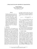
Illustrative example of the discretization processFigure 1
Illustrative example of the discretization process. This figure shows: (Left) Original expression matrix A'; and (Right)
Discretized matrix A obtained by considering a simple discretization technique, which uses a three symbol alphabet Σ = {D, N,
U}. The symbols mean down-regulation (D), up-regulation (U) or no-change (N). In this case, the values ∈ ]-0.3, 0.3[ were
discretized to N, and the values ≤ -0.3 and ≥ 0.3 were discretized to D and U, respectively.
C1 C2 C3 C4 C5
G1 0.07 0.73 -0.54 0.45 0.25
G2
-0.34 0.46 -0.38 0.76 -0.44
G3
0.22 0.17 -0.11 0.44 -0.11
G4
0.70 0.71 -0.41 0.33 0.35
G5
0.70 0.17 0.70 - 0.33 0.75
C1 C2 C3 C4 C5
G1 NUDUN
G2
DUDUD
G3
NNNUN

G4
UUDUU
G5
UDUDU
′
A
ij
′
A
ij
′
A
ij
Algorithms for Molecular Biology 2009, 4:8 />Page 4 of 39
(page number not for citation purposes)
Definition 4 (row-maximal CCC-Bicluster) A CCC-
Bicluster A
IJ
is row-maximal if we cannot add more rows to I
and maintain the coherence property referred in Definition 3.
Definition 5 (left-maximal and right-maximal CCC-
Bicluster) A CCC-Bicluster A
IJ
is left-maximal/right-maximal
if we cannot extend its expression pattern S to the left/right by
adding a symbol (contiguous column) at its beginning/end
without changing its set of rows I.
Definition 6 (maximal CCC-Bicluster) A CCC-Bicluster
A
IJ

is maximal if no other CCC-Bicluster exists that properly
contains A
IJ
, that is, if for all other CCC-Biclusters A
LM
, I ⊆ L
∧ J ⊆ M ⇒ I = L ∧ J = M.
Lemma 1 Every maximal CCC-Bicluster is right, left and row-
maximal.
Figure 2 shows the maximal CCC-Biclusters with at least
two rows (genes) present in the discretized matrix in Fig-
ure 1. CCC-Biclusters with only one row, even when max-
imal, are trivial and uninteresting from a biological point
of view and are thus discarded.
Maximal CCC-Biclusters and generalized suffix trees
Consider the discretized matrix A obtained from matrix A'
using the alphabet Σ. Consider also the matrix obtained
by preprocessing A using a simple alphabet transforma-
tion, that appends the column number to each symbol in
the matrix (see Figure 3), and considers a new alphabet Σ'
= Σ × {1, , |C|}, where each element Σ' is obtained by
concatenating one symbol in Σ and one number in the
range {1, , |C|}. We present below the two Lemmas and
the Theorem describing the relation between maximal
CCC-Biclusters with at least two rows and nodes in the
generalized suffix tree built from the set of strings
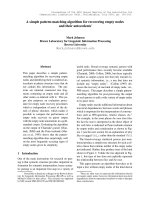
Maximal CCC-Biclusters in a discretized matrixFigure 2
Maximal CCC-Biclusters in a discretized matrix. This figure shows all maximal CCC-Biclusters with at least two rows
that can be identified in the discretized matrix in Figure 1. The strings S
B1

= [U], S
B2
= [U], S
B3
= [UN], S
B4
= [UDU], S
B5
= [U] and
S
B6
= [N] correspond to the expression patterns of the maximal CCC-Biclusters identified as B1, B2, B3, B4, B5 and B6, respec-
tively.
Algorithms for Molecular Biology 2009, 4:8 />Page 5 of 39
(page number not for citation purposes)
obtained after alphabet transformation [9,22]. Figure 4
illustrates this relation using the generalized suffix tree
obtained from the rows in the discretized matrix after
alphabet transformation in Figure 3 together with the
maximal CCC-Biclusters with at least two rows (B1 to B6)
already showed in Figure 2.
Lemma 2 Every right-maximal, row-maximal CCC-Bicluster
with at least two rows corresponds to one internal node in T and
every internal node in T corresponds to one right-maximal, row-
maximal CCC-Bicluster with at least two rows.
Lemma 3 An internal node in T corresponds to a left-maximal
CCC-Bicluster iff it is a MaxNode.
Definition 7 (MaxNode) An internal node v in T is called a
MaxNode iff it satisfies one of the following conditions:
a) It does not have incoming suffix links.

b) It has incoming suffix links only from nodes u
i
such that,
for every node u
i
, the number of leaves in the subtree rooted
at u
i
is inferior to the number of leaves in the subtree rooted
at v.
Theorem 1 Every maximal CCC-Bicluster with at least two
rows corresponds to a MaxNode in the generalized suffix tree T,
and each MaxNode defines a maximal CCC-Bicluster with at
least two rows.
Note that this theorem is the base of CCC-Biclustering
[9,22], which finds and reports all maximal CCC-Biclus-
ters using three main steps:
1. All internal nodes in the generalized suffix tree are
marked as "Valid", meaning each of them identifies a
row-maximal, right-maximal CCC-Bicluster with at
least two nodes according to Lemma 2.
2. All internal nodes identifying non left-maximal
CCC-Biclusters are marked as "Invalid" using Theorem
1, discarding all row-maximal, right-maximal CCC-
Biclusters which are not left-maximal.
3. All maximal CCC-Biclusters, identified by each
node marked as "Valid", are reported.
Methods
In this section we propose e-CCC-Biclustering, an algo-
rithm designed to find and report all maximal CCC-

Biclusters with approximate expression patterns (e-CCC-
Biclusters) using a discretized matrix A and efficient string
processing techniques. We first define the concepts of e-
CCC-Bicluster and maximal e-CCC-Bicluster. We then for-
mulate two problems: (1) finding all maximal e-CCC-
Biclusters and (2) finding all maximal e-CCC-Biclusters
satisfying row and column quorum constraints. We dis-
cuss the relation between maximal e-CCC-Biclusters and
generalized suffix trees highlighting the differences
between this relation and that of maximal CCC-Biclusters
and generalized suffix tree, discussed in the previous sec-
tion. We then discuss and explore the relation between the
two problems above and the Common Motifs Problem
[25,26]. We describe e-CCC-Biclustering, a polynomial
time algorithm designed to solve both problems and
sketch the analysis of its computational complexity. We
present extensions to handle missing values, discover
anticorrelated and scaled expression patterns, and con-
sider alternative ways to compute approximate expression
patterns. Finally, we propose a scoring criterion for e-
CCC-Biclusters combining the statistical significance of
their expression patterns with a similarity measure
between overlapping biclusters.
Illustrative example of the alphabet transformation performed after the discretization processFigure 3
Illustrative example of the alphabet transformation performed after the discretization process. This figure
shows: (Left) Discretized matrix A in Figure 1; (Right) Discretized matrix A after alphabet transformation.
C1 C2 C3 C4 C5
G1 NUDUN
G2
DUDUD

G3
NNNUN
G4
UUDUU
G5
UDUDU
C1 C2 C3 C4 C5
G1 N1 U2 D3 U4 N5
G2
D1 U2 D3 U4 D5
G3
N1 N2 N3 U4 N5
G4
U1 U2 D3 U4 U5
G5
U1 D2 U3 D4 U5
Algorithms for Molecular Biology 2009, 4:8 />Page 6 of 39
(page number not for citation purposes)
Figure 4 (see legend on next page)
Algorithms for Molecular Biology 2009, 4:8 />Page 7 of 39
(page number not for citation purposes)
CCC-Biclusters with approximate expression patterns
The CCC-Biclusters defined in the previous section are per-
fect, in the sense that they do not allow errors in the
expression pattern S that defines the CCC-Bicluster. This
means that all genes in I share exactly the same expression
pattern in the time points in J. Being able to find all max-
imal CCC-Biclusters using efficient algorithms is useful to
identify potentially interesting expression patterns and
can be used to discover regulatory modules [9]. However,

some genes might not be included in a CCC-Bicluster of
interest due to errors. These errors may be measurement
errors, inherent to microarray experiments, or discretiza-
tion errors, introduced by poor choice of discretization
thresholds or inadequate number of discretization sym-
bols. In this context, we are interested in CCC-Biclusters
with approximate expression patterns, that is, biclusters
where a certain number of errors is allowed in the expres-
sion pattern S that defines the CCC-Bicluster. We intro-
duce here the definitions of e-CCC-Bicluster and maximal
e-CCC-Bicluster preceded by the notion of e-neighbor-
hood:
Definition 8 (e-Neighborhood) The e-Neighborhood of a
string S of length |S|, defined over the alphabet
Σ
with |
Σ
| sym-
bols, N(e, S), is the set of strings S
i
, such that: |S| = |S
i
| and
Hamming(S, S
i
) ≤ e, where e is an integer such that e ≥ 0. This
means that the Hamming distance between S and S
i
is no more
than e, that is, we need at most e symbol substitutions to obtain

S
i
from S.
Lemma 4 The e-Neighborhood of a string S, N(e, S), contains
elements.
Definition 9 (e-CCC-Bicluster) A contiguous column coher-
ent bicluster with e errors per gene, e-CCC-Bicluster, is a CCC-
Bicluster A
IJ
where all the strings S
i
that define the expression
pattern of each of the genes in I are in the e-Neighborhood of
an expression pattern S that defines the e-CCC-Bicluster: S
i
∈
N (e, S), ∀i ∈ I. The definition of 0-CCC-Bicluster is equiva-
lent to that of a CCC-Bicluster.
Definition 10 (maximal e-CCC-Bicluster) An e-CCC-
Bicluster A
IJ
is maximal if it is row-maximal, left-maximal and
right-maximal. This means that no more rows or contiguous
columns can be added to I or J, respectively, maintaining the
coherence property in Definition 9.
Given these definitions we can now formulate the prob-
lem we solve in this work:
Problem 1 Given a discretized expression matrix A and
the integer e ≥ 0 identify and report all maximal e-CCC-
Biclusters .

Similarly to what happened with CCC-Biclusters, e-CCC-
Biclusters with only one row should be overlooked. A sim-
ilar problem is that of finding and reporting only the max-
imal e-CCC-Biclusters satisfying predefined row and
column quorum constraints:
Problem 2 Given a discretized expression matrix A and
three integers e
≥
0, q
r
≥ 2 and q
c
≥ 1, where q
r
is the row
quorum (minimum number of rows in I
k
) and q
c
is the
column quorum (minimum number of columns in J
k
),
identify and report all maximal e-CCC-Biclusters
such that, I
k
and J
k
have at least q
r

rows and q
c
columns, respectively.
Figure 5 shows all maximal e-CCC-Biclusters with at least
rows (genes), which are present in the discretized matrix
in Figure 1, when one error per gene is allowed (e = 1). Fig-
ure 6 shows all maximal e-CCC-Biclusters identified using
row and column constraints. In this case, the maximal 1-
CCC-Biclusters having at least three rows and three col-
umns (q
r
= q
c
= 3) are shown. Also clear in these figures is
the fact that, when errors are allowed (e > 0), different
expression patterns S can define the same e-CCC-Biclus-
ter. Furthermore, when e > 0, an e-CCC-Bicluster can be
defined by an expression pattern S, which does not occur
CS
j
S
jee
j
e
||
(| | ) | | | |ΣΣ−≤
=
∑
1
0

BA
kIJ
kk
=
BA
kIJ
kk
=
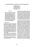
Maximal CCC-Biclusters and generalized suffix treesFigure 4 (see previous page)
Maximal CCC-Biclusters and generalized suffix trees. This figure shows: (Top) Generalized suffix tree constructed for
the transformed matrix in Figure 3. For clarity, this figure does not contain the leaves that represent string terminators that are
direct daughters of the root. Each internal node, other than the root, is labeled with the number of leaves in its subtree. We
show the suffix links between nodes although (for clarity) we omit the suffix links pointing to the root. All maximal CCC-
Biclusters are identified using a circle. The labels B1 to B6 identify the nodes corresponding to all maximal CCC-Biclusters with
at least two rows/genes. Note that the rows in each CCC-Bicluster identified by a given node v are obtained from the string
terminators in its subtree. The value of the string-depth of v and the first symbol in the string-label of v provide the information
needed to identify the set of contiguous columns. (Bottom) Maximal CCC-Biclusters B1 to B6 showed in the discretized
matrix as subsets of rows and columns. The strings S
B1
= [U], S
B2
= [U], S
B3
= [U N], S
B4
= [U D U], S
B5
= [U] and S
B6
= [N] cor-

respond to the expression patterns of the maximal CCC-Biclusters identified as B1 to B6, respectively.
Algorithms for Molecular Biology 2009, 4:8 />Page 8 of 39
(page number not for citation purposes)
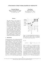
Maximal e-CCC-Biclusters in a discretized matrixFigure 5
Maximal e-CCC-Biclusters in a discretized matrix. This figure shows all maximal 1-CCC-Biclusters with at least two
rows that can be identified in the discretized matrix in Figure 1. Note that several of these 1-CCC-Biclusters can be defined by
more than one expression pattern. For example, B1 can be defined by S
B1
= [D], as shown in the figure, but can also be defined
by S
B1
= [N] or S
B1
= [U]. Other 1-CCC-Biclusters are defined by expression patterns not occurring in the discretized matrix
in the contiguous columns identifying the biclusters. This is the case of 1-CCC-Bicluster B2, for example, defined by the pattern
S
B2
= [D D], which does not occur in the columns C1–C2.
Algorithms for Molecular Biology 2009, 4:8 />Page 9 of 39
(page number not for citation purposes)
in the discretized matrix in the set of contiguous columns
in the e-CCC-Bicluster.
Maximal e-CCC-Biclusters and generalized suffix trees
In the previous section we showed that each internal node
in the generalized suffix tree, constructed for the set of
strings corresponding to the rows in the discretized matrix
after alphabet transformation, identifies exactly one CCC-
Bicluster with at least two rows (maximal or not) (see
Lemma 2). We also showed that each internal node corre-
sponding to a MaxNode (see Definition 7) in the general-

ized suffix tree identifies exactly one maximal CCC-
Bicluster and that each maximal CCC-Bicluster is identi-
fied by exactly one MaxNode (see Lemma 3 and Theorem
1). This also implies that a maximal CCC-Bicluster is iden-
tified by one expression pattern, which is common to all
genes in the CCC-Bicluster within the contiguous col-
umns in the bicluster. Moreover, all expression patterns
identifying maximal CCC-Biclusters always occur in the
discretized matrix and thus correspond to a node in the
generalized suffix tree (see Figure 4).
When errors are allowed, one e-CCC-Bicluster (e > 0) can
be identified (and usually is) by several nodes in the gen-
Maximal e-CCC-Biclusters with row and column quorum constraints in a discretized matrixFigure 6
Maximal e-CCC-Biclusters with row and column quorum constraints in a discretized matrix. This figure shows
the five maximal 1-CCC-Biclusters with at least 3 rows/columns (q
r
= q
c
= 3) that can be identified in the discretized matrix in
Figure 1. These 1-CCC-Biclusters are defined, respectively, by the following patterns: S
B1
= [D U D U], S
B2
= [D D U], S
B3
= [D
U N], S
B4
= [N D U] and S
B5

= [U D U D]. Also clear from this figure is the fact that the same e-CCC-Bicluster can be defined
by several patterns. For example, 1-CCC-Bicluster B1 can also be identified by the patterns [N U D U] and [U U D U]. An
interesting example is the case of 1-CCC-Bicluster B2, which can also be defined by the patterns [N D U], [U N U], [U U U],
[U D D] and [U D N]. Note however, that B2 cannot be identified by the pattern [U D U]. If this was the case, B2 would not
be right maximal, since the pattern [U D N] can be extended to the right by allowing one error at column 5. In fact, this leads
to the discovery of the maximal 1-CCC-Bicluster B5. Moreover, e-CCC-Biclusters can be defined by expression patterns not
occurring in the discretized matrix. This is the case of 1-CCC-Biclusters B2 and B4, defined respectively by the patterns S
B2
=
[D D U] and S
B4
= [N D U], which do not occur in the matrix in the contiguous columns defining B2 and B4 (C2–C3 and C2–
C4, respectively).
Algorithms for Molecular Biology 2009, 4:8 />Page 10 of 39
(page number not for citation purposes)
eralized suffix tree, constructed for the set of strings corre-
sponding to the rows in the discretized matrix after
alphabet transformation, and one node in the generalized
suffix tree may be related with multiple e-CCC-Biclusters
(maximal or not) (see Figure 7). Moreover, a maximal e-
CCC-Bicluster can be defined by several expression pat-
terns (see Figure 5 and Figure 6). Upon all this, a maximal
e-CCC-Bicluster can be defined by an expression pattern
not occurring in the expression matrix and thus not appear-
ing in the generalized suffix tree (see Figure 6 and Figure
7).
Furthermore we cannot obtain all maximal e-CCC-Biclus-
ters using the set of maximal CCC-Biclusters by: 1) extend-
ing them with genes by looking for their approximate
patterns in the generalized suffix tree, or 2) extending

them with e contiguous columns (see Figure 5 and Figure
8). It is also clear from Figure 8 that extending maximal
CCC-Biclusters can in fact lead to the discovery of non
maximal e-CCC-Biclusters. For the reasons stated above
we cannot use the same searching strategy used to find
maximal CCC-Biclusters when looking for maximal e-
CCC-Biclusters (e > 0). We therefore need to explore the
relation between finding e-CCC-Biclusters and the Com-
mon Motifs Problem, as explained below.
Finding e-CCC-Biclusters and the common motifs problem
There is an interesting relation between the problem of
finding all maximal e-CCC-Biclusters, discussed in this
work, and the well known problem of finding common
motifs (patterns) in a set of sequences (strings). For the
first problem, and to our knowledge, no efficient algo-
rithm has been proposed to date. For the latter problem
(Common Motifs Problem), several efficient algorithms
based on string processing techniques have been pro-
posed to date [25,26]. The Common Motifs Problem is as
follows [26]:
Common Motifs Problem Given a set of N sequences S
i
(1 ≤ i ≤ N) and two integers e ≥ 0 and 2 ≤ q ≤ N, where e is
the number of errors allowed and q is the required quo-
rum, find all models m that appear in at least q distinct
sequences of S
i
.
During the design of e-CCC-Biclustering, we used the
ideas proposed in SPELLER [26], an algorithm to find

common motifs in a set of N sequences using a generalized
suffix tree T. The motifs searched by SPELLER correspond
to words, over an alphabet Σ, which must occur with at
most e mismatches in 2 ≤ q ≤ N distinct sequences. Since
these words representing the motifs may not be present
exactly in the sequences (see SPELLER for details), a motif
is seen as an "external" object and called model. In order to
be considered a valid model, a given model m of length |m|
has to verify the quorum constraint: m must belong to the e-
neighborhood of a word w in at least q distinct sequences.
In order to solve the Common Motifs Problem, SPELLER
builds a generalized suffix tree T for the set of sequences S
i
and then, after some further preprocessing, uses this tree
to "spell" the valid models. Valid models verify two prop-
erties [26]:
1. All the prefixes of a valid model are also valid mod-
els.
2. When e = 0, spelling a model leads to one node v in
T such that L(v) ≥ q, where L(v) denotes the number of
leaves in the subtree rooted at v.
When e > 0, spelling a model leads to a set of nodes v
1
,
, v
k
in T for which , where L(v
j
)
denotes the number of leaves in the subtree rooted at

v
j
.
In these settings, and since the occurrences of a model are
in fact nodes of the generalized suffix tree T, these occur-
rences are called node-occurrences [26]. The goal of
SPELLER is thus to identify all valid models by extending
them in the generalized suffix tree and to report them
together with their set of node-occurrences. We present
here an adaptation of the definition of node-occurrence
used in SPELLER. In SPELLER, a node-occurrence is
defined by a pair (v, v
err
) and not by a triple (v, v
err
, p), as
in this work. For clarity, SPELLER was originally exempli-
fied [26] in an uncompacted version of the generalized
suffix tree, that is, a trie (although it was proposed to work
with a generalized suffix tree). However, and as pointed
out by the authors, when using a generalized suffix tree, as
in our case, we need to know at any given step in the algo-
rithm whether we are at a node or in an edge between
nodes v and v'. We use p to provide this information, and
redefine node-occurrence as follows:
Definition 11 (node-occurrence) A node-occurrence of a
model m is a triple (v, v
err
, p), where v is a node in the gener-
alized suffix tree T and v

err
is the number of mismatches
between m and the string-label of v computed using Ham-
ming(m, string-label(v)). The integer p ≥ 0 identifies a posi-
tion/point in T such that:
1. If p = 0: we are exactly at node v.
2. If p > 0: we are in E(v), the edge between father
v
and v,
in a point p between two symbols in label(E(v)) such that 1
≤ p < |label(E(v))|.
Lv q
j
j
k
()≥
=
∑
1
Algorithms for Molecular Biology 2009, 4:8 />Page 11 of 39
(page number not for citation purposes)
Figure 7 (see legend on next page)
Algorithms for Molecular Biology 2009, 4:8 />Page 12 of 39
(page number not for citation purposes)
Consider a model m, a symbol
α
in the alphabet Σ, a node
v in T, its father father
v
, the edge between father

v
and v,
E(v), the edge-label of E(v), label(E(v)) and its edge-
length, |label(E(v))|. The modified version of SPELLER
described below is based on the following Lemmas
(adapted from SPELLER):
Lemma 5 (v, v
err
, 0) is a node-occurrence of a model m' = m
α
,
if, and only if:
1. Match:
(father
v
, v
err
, 0) is a node-occurrence of m and
label(E(v)) =
α
.
The edge-label of E(v) has only one symbol and this
symbol is
α
.
or
(v, v
err
, |label(E(v))| -1) is a node-occurrence of m and
label(E(v)) [|label(E(v))|] =

α
.
The last symbol in label(E(v)) is
α
.
2. Substitution:
(father
v
, v
err
-1, 0) is a node-occurrence of m and
label(E(v)) =
β
≠
α
.
The edge-label of E(v) has only one symbol and this
symbol is not
α
.
or
(v, v
err
- 1, |label(E(v))| - 1) is a node-occurrence of m
and label(E(v)) [|label(E(v))|] =
β
≠
α
.
The last symbol in label(E(v)) is not

α
.
Lemma 6 (v, v
err
, 1) is a node-occurrence of a model m' = m
α
,
if, and only if:
1. Match:
(father
v
, v
err
, 0) is a node-occurrence of m and
label(E(v))[1] =
α
.
2. Substitution:
(father
v
, v
err
- 1, 0) is a node-occurrence of m and
label(E(v))[1] =
β
≠
α
.
Lemma 7 (v, v
err

, p), 2 ≤ p < |label(E(v)| is a node-occurrence
of a model m' = m
α
, if, and only if:
1. Match:
(v, v
err
, p - 1) is a node-occurrence of m and label(E(v)
[p] =
α
.
2. Substitution:
(v, v
err
- 1, p - 1) is a node-occurrence of m and
label(E(v)) [p] =
β
≠
α
.
Consider now the discretized matrix A obtained from
matrix A' using the alphabet Σ. We preprocess A using the
same alphabet transformation used in CCC-Biclustering.
Remember that we append the column number to each
symbol in the matrix and consider a new alphabet Σ' = Σ
× {1, , |C|} (see Figure 3). We will now show that
SPELLER can be adapted to extract all right-maximal e-
CCC-Biclusters from this transformed matrix A by build-
ing a generalized suffix tree for the set of |R| strings S
i

obtained from each row in A and use it to "spell" the valid
models using the symbols in the new alphabet Σ'.
Given the set of |R| strings S
i
, the number of allowed
errors e ≥ 0 and the quorum constraint 2 ≤ q ≤ |R|, the goal
is now to find the set of all right-maximal valid models m,
identifying expression patterns that are present in at least
q distinct rows starting and ending at the same columns. Note
that the valid models identified by the original SPELLER
algorithm are already row-maximal. However they may be
e-CCC-Biclusters (e > 0) and generalized suffix treesFigure 7 (see previous page)
e-CCC-Biclusters (e > 0) and generalized suffix trees. This figure shows: (Top) Generalized suffix tree constructed for
the transformed matrix in Figure 3 (the information stored in the nodes correspond to the number of leaves and row identifi-
ers in their subtree and is used by e-CCC-Biclustering). The circles labeled with B1, B2, B3, B4 and B5 identify the nodes
related with the five maximal 1-CCC-Biclusters discovered when e = 1 and q
e
= q
c
= 3, shown in Figure 6; (Bottom) Maximal
1-CCC-Biclusters B1 to B5 showed in the matrix as subsets of rows and columns. The strings S
B1
= [D U D U], S
B2
= [D D U],
S
B3
= [D U N], S
B4
= [N D U] and S

B5
= [U D U D] correspond to the expression patterns defining the maximal 1-CCC-Biclus-
ters identified as B1 to B5, respectively. Note that e-CCC-Biclusters can now be identified (and generally are) by more than
one node in the generalized suffix tree. This is the case of 1-CCC-Biclusters B1, B3, B4 and B5. In fact only B2 is identified by a
single node in this example. Moreover, a node in the generalized suffix tree might be related with more than one maximal e-
CCC-Bicluster. Look for example at the node identifying approximate patterns occurring in both 1-CCC-Biclusters B2 and B4.
Algorithms for Molecular Biology 2009, 4:8 />Page 13 of 39
(page number not for citation purposes)
Figure 8 (see legend on next page)
Algorithms for Molecular Biology 2009, 4:8 />Page 14 of 39
(page number not for citation purposes)
non right-maximal, non left-maximal, and start at differ-
ent positions in the sequences. Under these settings, the
set of node-occurrences of each valid model m and the
model itself in our modified version of SPELLER identifies
one row-maximal, right-maximal e-CCC-Bicluster with q
rows and a maximum of |C| contiguous columns. Further-
more, it is possible to find all right-maximal e-CCC-
Biclusters by fixing the quorum constraint, used to specify
the number of rows/genes necessary to identify a model as
valid, to the value q = 2. In this context, and in order to be
able to solve not only Problem 1 but also Problem 2, we
adapted SPELLER to consider not only a row constraint, 2 ≤
q
r
≤ |R|, but also an additional column constraint, 1 ≤ q
c
≤
|C|.
Figure 7 shows the generalized suffix tree used by our

modified version of SPELLER when it is applied to the dis-
cretized matrix after alphabet transformation in Figure 3.
We can also see in this figure the five maximal 1-CCC-
Biclusters B1, B2, B3, B4 and B5, already shown in Figure
6, identified by five valid models, when e = 1 and the val-
ues q
r
and q
c
, specifying the row and column constraints,
respectively, are set to 3. The maximal 1-CCC-Biclusters
B1 to B5 are defined, respectively, by the following valid
models: m = [D1 U2 D3 U4 N5] (three node-occurrences
labeled with B1); m = [D2 D3 U4] (three node-occur-
rences labeled with B2), m = [D3 U4 N5] (four node-
occurrences labeled with B3), m = [N2 D3 U4] (four node-
occurrences labeled with B4) and m = [U2 D3 U4 D5]
(four node-occurrences labeled with B5). It is also possi-
ble to observe in this figure that, when e > 0, a model can
be valid without being right/left-maximal and that several
valid models may identify the same e-CCC-Bicluster. For
example, m = [D1 U2 D3] is valid but it is not right-maxi-
mal, m = [D3 U4 D5] is also valid but it is not left-maxi-
mal, and finally the models m = [D1 U2 D3 U4 N5] and
m = [N1 U2 D3 U4 D5] are both valid but identify the
same 1-CCC-Bicluster B1. Figure 4 shows the generalized
suffix tree used when e = 0, q
r
= 2 and q
c

= 1. Since no errors
are allowed the generalized suffix tree is the same as the
one used by CCC-Biclustering and the maximal 0-CCC-
Biclusters identified correspond in fact to the maximal
CCC-Biclusters in Figure 2.
In the next section we describe the details of the modified
version of SPELLER that we used to identify all right-max-
imal e-CCC-Biclusters. However, and for clarity, we sum-
marize here the main differences between the original
version of SPELLER and the modified version (procedure
computeRightMaximalBiclusters in the next sec-
tion), which we use as the first step of the e-CCC-Biclus-
tering algorithm. While reading the differences listed
below have in mind that in order to be maximal, an e-
CCC-Bicluster must be row-maximal, right-maximal and
left-maximal. Moreover, all the approximate patterns
identifying genes in an e-CCC-Bicluster must start and end
at the same columns.
1. In SPELLER a node-occurrence is defined by a pair
(v, v
err
) since (for clarity) the algorithm was exempli-
fied using a trie and not a generalized suffix tree, as
explained above. As such we redefined the original
concept of node-occurrence to use the triple (v, v
err
, p)
(see Definition 11), adapted the three original Lem-
mas in SPELLER to use the new definition of node-
occurrence (see Lemma 5, Lemma 6 and Lemma 7),

and rewrote SPELLER to use a generalized suffix tree.
2. In SPELLER a model can be valid without being
right/left-maximal. As such all models satisfying the
quorum constraint are stored for further reporting.
This means that the valid models reported by SPELLER
are only row-maximal. We only store valid models
that cannot be extended to the right without loosing
Maximal CCC-Biclusters and maximal e-CCC-BiclustersFigure 8 (see previous page)
Maximal CCC-Biclusters and maximal e-CCC-Biclusters. This figure shows: (Top) 1-CCC-Biclusters obtained from
the maximal CCC-Biclusters in Figure 2 by extending them with genes by looking for their approximate patterns in the gener-
alized suffix tree (1-CCC-Biclusters B1_1, B2_1, B3_1, B5_1 and B6_1) or extending them with e = 1 contiguous columns at
right (1-CCC-Biclusters B1_2, B1_3, B2_2, B4_2, B6_2 and B6_3) or at left (1-CCC-Biclusters B2_3, B3_2, B4_1, B5_2 and
B5_3). Note that several of these 1-Biclusters can be defined by more than one expression pattern. This is the case of 1-CCC-
Biclusters B2_1, B2_3, B3_2, B4_1 and B4_2, which in fact correspond to maximal 1-CCC-Biclusters (see Figure 5). Other 1-
CCC-Biclusters are identified by a single expression pattern. This is the case of 1-CCC-Biclusters B1_1, B1_2, B2_1, B3_1,
B5_1, B5_2, B6_1 and B6 2, and also correspond to maximal 1-CCC-Biclusters (see Figure 5). However, the 1-CCC-Biclusters
B1_3, B5_3 and B6_3 do not correspond to maximal 1-CCC-Biclusters since they are not row-maximal. (Bottom) Maximal
1-CCC-Biclusters B1_3, B5_3 and B6_3 obtained not only by extending maximal CCC-Biclusters B1, B5 and B6 with one con-
tiguous column to the right, left and right, respectively, but also by looking for the patterns in the 1-neighborhood of the pat-
terns S
B1_3
= [U U] (columns C1–C2), S
B5_3
= [U U] (columns C4–C5) and S
B6_3
= [N U] (columns C1–C2). Note however, that
even if we replaced the non maximal 1-CCC-Biclusters B1_3, B5_3 and B6_3 (in the top) by the truly maximal 1-CCC-Biclus-
ters (in the bottom) we could only find 16 of the 36 maximal 1-CCC-Biclusters with at least two rows shown in Figure 5 that
can be found in the discretized matrix in Figure 1.
Algorithms for Molecular Biology 2009, 4:8 />Page 15 of 39

(page number not for citation purposes)
genes, that is valid models which are both row-maxi-
mal are right-maximal. This implied modifying the
original procedure storeModel in SPELLER in order
to include the procedure checkRightMaximality
(see procedure spellModels in the next section, for
details).
3. In SPELLER the node-occurrences of a valid model
can start in any position in the sequences. In our mod-
ified version of this algorithm all node-occurrences of
a valid model must start in the same position (same
column in the discretized matrix) in order to guaran-
tee that they belong to an e-CCC-Bicluster. As such we
modified the construction of the generalized suffix
tree used in SPELLER in order to be constructed using
the set of strings corresponding to the set of rows in
the discretized matrix after alphabet transformation.
We also modified all the procedures used in SPELLER
for model extension. Note that it is not possible to
modify SPELLER in order to check if a valid model that
is right-maximal is also left-maximal. This is so since
we can only guarantee that a model is/is not left-max-
imal once we have computed all valid models corre-
sponding to right-maximal e-CCC-Biclusters. This
justifies why we need to discard valid models which
are not left-maximal in the next step of the algorithm
and did not integrate this step in our modified version
of SPELLER.
In this context, we also show in the next section that the
proposed e-CCC-Biclustering algorithm will need three

steps to identify all maximal e-CCC-Biclusters without rep-
etitions: a first step to identify all right-maximal e-CCC-
Biclusters (for this we use the modified version of
SPELLER), a second step to discard all right-maximal e-
CCC-Biclusters which are not left-maximal, and finally a
third step to discard repetitions, that is maximal valid
models identifying the same maximal e-CCC-Bicluster.
Note that the original SPELLER algorithm does not elimi-
nate repetitions (different valid models with the same set
of node-occurrences). Furthermore, we also cannot inte-
grate the elimination of valid models corresponding to
the same right-maximal e-CCC-Biclusters in our modified
version of SPELLER since we need the set of all valid mod-
els corresponding to right-maximal e-CCC-Biclusters in
order to discard valid models which are not left-maximal
in the second step of e-CCC-Biclustering.
e-CCC-Biclustering: Finding and reporting all maximal e-
CCC-Biclusters in polynomial time
This section presents e-CCC-Biclustering, a polynomial
time biclustering algorithm for finding and reporting all
maximal CCC-Biclusters with approximate patterns (e-
CCC-Biclusters), and describes its main steps. Algorithm 1
is designed to solve Problem 2: identify and report all
maximal e-CCC-Biclusters such that I
k
and J
k
have at least q
r
rows and q

c
columns, respectively. The pro-
posed algorithm is easily adapted to solve problem 1
(identify and report all maximal e-CCC-Biclusters
without quorum constraints) by fixing the val-
ues of q
r
and q
c
to the values two and one, respectively. The
proposed algorithm is based on the following steps
(described in detail below):
[Step 1] Computes all valid models corresponding to
right-maximal e-CCC-Biclusters. Uses the discretized
matrix A after alphabet transformation, the quorum
constraints q
r
and q
c
, a generalized suffix tree and a
modified version of SPELLER.
[Step 2] Deletes all valid models not corresponding to
left-maximal e-CCC-Biclusters. Uses all valid models
computed in Step 1 and a trie.
[Step 3] Deletes all valid models representing the
same e-CCC-Biclusters. Uses all valid models corre-
sponding to maximal e-CCC-Biclusters (both left and
right) computed in Step 2 and a hash table. Note that
this step is only needed when e > 0.
[Step 4] Reports all maximal e-CCC-Biclusters.

Algorithm 1: e-CCC-Biclustering
Input : A, Σ, e, q
r
, q
c
Output: Maximal e-CCC-Biclusters.
1 {S
1
, , S
|R|
} ← alphabetTransformation(A, Σ)
2 modelsOcc
←
{}
3 computeRightMaximalBiclusters(Σ, e, q
r
, q
c
, {S
1
,
, S
|R|
}, modelsOcc)
4 deleteNonLeftMaximalBiclusters(modelsOcc)
5 if e > 0 then
6 deleteRepeatedBiclusters(modelsOcc)
7 reportMaximalBiclusters(modelsOcc)
Detailed discussions can be found in additional file 2:
algorithmic_complexity_details.

BA
kIJ
kk
=
BA
kIJ
kk
=
Algorithms for Molecular Biology 2009, 4:8 />Page 16 of 39
(page number not for citation purposes)
Computing valid models corresponding to right-maximal e-CCC-
Biclusters
In step 1 of e-CCC-Biclustering we compute all valid mod-
els m together with their node-occurrences Occ
m
corre-
sponding to right-maximal e-CCC-Biclusters. The details
are shown in the procedure computeRightMaximal
Biclusters below, which corresponds to a modified
version of SPELLER.
Procedure computeRightMaximalBiclusters
Input: Σ, e, q
r
, q
c
, {S
1
, , S
|R|
}, modelsOcc

/* The value of modelsOcc is updated.*/
1 T
right
← constructGeneralizedSuffixTree({S
1
,
, S
|R|
})
2 addNumberOfLeaves(T
right
) /* Adds L(v) to each
node v in T
right
.*/
3 if e ≠ 0 then
4 addColorArray(T
right
)
/* Adds colors
v
to every node v in T
right
: colors
v
[i]
= 1, if there is a leaf in the subtree rooted
at v that is a suffix ofS
i
; colors

v
[i] = 0,
otherwise.*/
5 m ← "" /* model m is a string [m [1] m [length
m
-
1]] */
6 length
m
← 0
7 father
m
← "" /* father
m
is a string [m[1] m
[length
m
-1]] */
8 ← 0
9 Occ
m
← {} /* List of node-occurrences (v, v
err
,
p)*/
10 addNodeOccurrence(Occ
m
, (root(T
right
), 0, 0))

11 Ext
m
← {} /* Ext
m
is the set of possible sym
bols
α
to extend the model m.*/
12 if e = 0 then
13 forall edges E(v
i
) leaving from node root(T
right
) to a node
v
i
do
14 if label(E(v
i
))[1]is not a string terminator then
15 addSymbol(Ext
m
, label(E(v
i
))[1])
16 else
17 forall symbols in
Σ
' do
/* Σ' must be in lexicographic

order.*/
18 addSymbol(Ext
m
,
Σ
' [i])
19 length
m
← 0
20 spellModels(Σ, e, q
r
, q
c
, modelsOcc, T
right
, m, length
m
,
Occ
m
, Ext
m
, father
m
, )
In this procedure we use the transformed matrix A as
input and store the results in the list modelsOcc, which
stores triples with the following information (m,
genesOcc
m

, numberOfGenesOcc
m
), where m is the model,
genesOcc
m
is a bit vector containing the distinct genes in
the node-occurrences of m, Occ
m
, and numberOfGenesOcc
m
is the number of bits set to 1 in genesOcc
m
and, therefore,
the number of genes where the model occurs. This infor-
mation is computed using the procedure spellModels
described below, which corresponds to a modified ver-
sion of the procedure with the same name used in
SPELLER).
Procedure spellModels
/* Called recursively. Stores right-max
imal e-CCC-Biclusters in modelsOcc.*/
Input : Σ, e, q
r
, q
c
, modelsOcc, T
right
, m, length
m
, Occ

m
,
Ext
m
, father
m
,
/* The value of modelsOcc is updated.*/
1 keepModel(q
r
, q
c
, modelsOcc, T
right
, m, length
m
, Occ
m
,
father
m
,
2 if length
m
≤ |C| then
/* |C| is the length of the longest
model */
3 forall symbols
α
in Ext

m
do
4if
α
is not a string terminator then
numberOfGenesOcc
father
m
numberOfGenesOcc
father
m
numberOfGenesOcc
father
m
numberOfGenesOcc
father
m
Algorithms for Molecular Biology 2009, 4:8 />Page 17 of 39
(page number not for citation purposes)
5 maxGenes ← 0/* Sum of L(v) for all node-
occurrences (v, v
err
, p) in Occ
m
α
*/
6 minGenes← ∞/* Minimum L(v) in all node-
occurrences (v, v
err
, p) in Occ

m
α
*/
7 Colors
m
α

← {}
8if e > 0 then
9 Colors
m
α

[i] ← 0, 1 ≤ i ≤ |R|
/* colors
m
α

[i] = 1, if there is a node-
occurrence of m in S
i
;*/
/* colors
m
α

[i] = 0, otherwise */
10 Ext
m
α

← {}
11 Occ
m
α

← {}
12 forall node-occurrences (v, v
err
, p) in Occ
m
do
/* If p = 0 we are at node v. Otherwise,
we are at edge E(v) between nodes father(v) andv
at point p > 0. */
13 if p = 0 then
14 extendFromNodeWithoutErrors(Σ, e,
T
right
, (v, v
err
, p), m,
α
, Occ
m
α
, Colors
m
α

, Ext
m
α
, maxGenes,
minGenes)
15 if (v
err
<e) then
16 extendFromNodeWithErrors(Σ, e, T
right
,
(v, v
err
, p), m,
α
, Occ
m
α

, Colors
m
α

, Ext
m
α
, maxGenes, min-
Genes)
17 else
18 extendFromEdgeWithoutErrors(T

right
,
Σ, e, (v, v
err
, p), m,
α
, m, Occ
m
α
, Colors
m
α

, Ext
m
α

, maxGenes,
minGenes)
19 if x
err
<e then
20 extendFromEdgeWithErrors(Σ, e, T
right
,
(v, v
err
, p), m,
α
, Occ

m
α

, Colors
m
α

, Ext
m
α
, maxGenes, min-
Genes)
21 if modelHasQuorum(maxGenes, minGenes, Color-
s
m
α
, q
r
) then
22 spellModels(Σ, e, q
r
, q
c
, modelsOcc, T
right
, m
α
,
length
m

+ 1, Occ
m
α

, Ext
m
α

, father
m
α
, numberOfGenesOcc
m
)
The recursive procedure spellModels (modified to
extract valid models corresponding to right-maximal e-
CCC-Biclusters) is now able to:
1. Use a generalized suffix tree T
right
and define node-
occurrences as triples (v, v
err
, p), where p is used
throughout the algorithm to find out whether we are
at node v (p = 0) or in an edge E(v) between nodes v
and father
v
(p > 0).
2. Check if a valid model m corresponds to a right-
maximal e-CCC-Bicluster. This is performed using the

procedure checkRightMaximality inside the pro-
cedure keepModel. This procedure deletes from the
list of stored models, modelsOcc, a valid model m when
the result of its extension with a symbol
α
, m
α
, is also
a valid model and the set of node-occurrences of m
α
,
Occ
m
α
, has as many genes as the set of node-occur-
rences of its father m, Occ
m
. When this is the case, m no
longer corresponds to a right-maximal e-CCC-Biclus-
ter since its expression pattern can be extended to the
right with the symbol
α
without losing genes.
3. Restrict the extensions of a given model m, Ext
m
, to
the level of the model in the generalized suffix tree
(column of the last symbol in m). When we are
extending a model m with a symbol
α

(eventually
extracting a valid model m
α
), the column number of
the last symbol in m, m [length
m
], is C(m [length
m
]),
where C(m [length
m
]) ∈ {1, , |C|}, and errors are still
allowed,
α
can only be one of the symbols in the set
, where corresponds to
the subset of elements in Σ' whose column is equal to
C(m [length
m
])) + 1. For example, if Σ = {D, N, U} and
the model m = [D1] is being extended, the possible
symbols
α
with which m can be extended to m
α
must
be in = {D2. N 2, U 2}. In the same way, if m = [D2
U3], the possible symbols
α
with which m can be

extended to m
α
are in = {D4, N 4, U 4}.
The algorithmic details of the procedures and functions
called in the recursive procedure spellModels are
described in additional file 2:
algorithmic_complexity_details.
′
+
Σ
Cmlength
m
([ ])1
′
+
Σ
Cmlength
m
([ ])1
′
Σ
2
′
Σ
4
Algorithms for Molecular Biology 2009, 4:8 />Page 18 of 39
(page number not for citation purposes)
Deleting valid models not corresponding to left-maximal e-CCC-
Biclusters
In step 2 of e-CCC-Biclustering (details in procedure

deleteNonLeftMaximalBiclusters below), we
remove from the valid models stored in modelsOcc (iden-
tifying right-maximal e-CCC-Biclusters) those not corre-
sponding to left-maximal e-CCC-Biclusters. These models
are removed from modelsOcc by first building a trie with
the reverse patterns of all (right-maximal) models m and
storing the number of genes in numberOfGenesOcc
m
in its
corresponding node in the trie. After this, it is sufficient to
mark as "non left-maximal" any node in the trie that has
at least one child with as many genes as itself. This is easily
achieved by performing a depth-first search (dfs) of the
trie and computing, for each node, the maximum value
amongst the values of numberOfGenesOcc
m
stored in its
children. The models whose corresponding node in the
trie is marked as "non left-maximal" are then removed
from modelsOcc.
Procedure deleteNonLeftMaximalBiclusters
Input: modelsOcc
/* The value of modelsOcc is updated. */
1 T
left
← createTrie ()
/* Array which will store references to
nodes in T
left
*/

2 R
nodes
← {}
3 foreach model and occurrences (m, genesOcc
m
, numberOf-
GenesOcc
m
) in modelsOcc do
4 m
r
← ReverseModel(m)
5 nodeRepresentingModel
←
addReverseModelToT
rie(T
left
, m
r
)
/* Each node in T
left
stores two integers1)
the number of genes in the model it rep
resents, genes
v
(0 if it does not represent
the end of a model); and 2) the maximum
number of genes in the subtree rooted atv,
(computed later). Both these

values are initialized with 0.*/
6 addNumberOfGenes(nodeRepresentingModel,number
OfGenesOcc
m
)
7 addReferenceToNode(R
nodes
, nodeRepresenting-
Model)
8 forall nodes v in T
left
do
/* Performed using a depth-first search
(dfs) */
9if genes
v
> 0 then
/* Node v represents a model and is
potentially left-maximal.*/
10 Mark v as "left-maximal"
11 else
12 Mark v as "non left-maximal"
13 Compute the maximum number of genes in the sub-
tree rooted at v
14 foreach node v in T
left
do
/* Performed using a depth-first search
(dfs) */
15 if genes

v
> 0 and genes
v
= then
16 Mark v as "non left-maximal"
17 p
modelsOcc
← 0
18 foreach model and occurrences (m, genesOcc
m
, numberOf-
GenesOcc
m
) in modelsOcc do
19 if R
nodes
[p
modelsOcc
] is marked as "non-left maximal" then
20 deleteModelAndOccurrences(modelsOcc, m)
21 p
modelsOcc
← p
modelsOcc
+ 1
Deleting valid models representing the same e-CCC-Biclusters
When errors are allowed, different valid models may iden-
tify the same e-CCC-Bicluster. Step 3 of e-CCC-Bicluster-
ing, described in detail in procedure
deleteRepeatedBiclusters below, uses a hash

table to remove from modelsOcc all the valid models that,
although maximal (left and right), identify repeated e-
CCC-Biclusters. This is needed because all valid models m
with the same first and last columns and the same set of
genes represent the same maximal e-CCC-Bicluster.
Procedure deleteRepeatedBiclusters
Input: modelsOcc
/* The value of modelsOcc is updated.*/
maxGenes
subtree
v
maxGenes
subtree
v
Algorithms for Molecular Biology 2009, 4:8 />Page 19 of 39
(page number not for citation purposes)
1 H
←
createHashTable()
2 foreach model and occurrences (m, genesOcc
m
, numberOf-
GenesOcc
m
) in modelsOcc do
3 firstColumn
m
= C(m [1])
4 lastColumn
m

= C(m [length
m
])
5 key ← createKey(firstColumn, lastColumn, genesOcc
m
)
6 value ← (firstColumn, lastColumn, genesOcc
m
)
7if containsKey(H, key) then
8 value
key
← getValue(H, key)
9if value = value
key
then
/* H already has a value representing
the same e-CCC-Bicluster */
10 deleteModelAndOccurrences(modelsOcc,
m)
11 else
12 insertKeyValue(key, value)
13 else
14 insertKeyValue(key, value)
Reporting all maximal e-CCC-Biclusters
After the three main steps of e-CCC-Biclustering the list
modelsOcc stores all valid models corresponding to maxi-
mal e-CCC-Biclusters satisfying the quorum constraints q
r
and q

c
. In this context, the reporting procedure report
MaximalBiclusters, described below, lists these e-
CCC-Biclusters using the information stored in the model
m (needed to identify the expression pattern and the col-
umns in each e-CCC-Bicluster) and the bit vector genesOcc
(needed to identify the genes in the e-CCC-Bicluster).
Procedure reportMaximalBiclusters
Input: modelsOcc
1 foreach model and occurrences (m, genesOcc
m
, numberOf-
GenesOcc
m
) in modelsOcc do
2 firstColumn
m
= C(m [1])
3 lastColumn
m
= C(m [length
m
])
4 print(m, firstColumn
m
, lastColumn
m
, genesOcc
m
)

e-CCC-Biclustering: Complexity analysis
In this section we sketch an analysis of the complexity of
e-CCC-Biclustering. For a detailed complexity analysis see
additional file 2: algorithmic_complexity_details.
Given a discretized matrix A with |R| rows and |C| col-
umns, the alphabet transformation performed using the
procedure alphabetTransformation takes O(|R||C|)
time.
The complexity of computing all valid models corre-
sponding to right-maximal e-CCC-Biclusters using proce-
dure computeRightMaximalBiclusters takes
O(|R|
2
|C|
1 + e
|Σ|
e
) operations. The construction of T
right
and the computation of L(v) for all its nodes takes
O(|R||C|) time each, using Ukkonen's algorithm with
appropriate data structures, and a dfs, respectively. The
increase in the alphabet size from |Σ| to |C||Σ| due to the
alphabet transformation does not affect the O(|R||C|)
construction and manipulation of the generalized suffix
tree [9]. When e > 0, adding the color array to all nodes in
T
right
takes O(|R|
2

|C|) time. Initializing Ext
m
takes
O(|C||Σ|) and spellModels is O(|R|
2
|C|
1 + e
|Σ|
e
). The
complexity of this step of the algorithm is bounded by the
complexity of spellModels and is thus
O(|R|
2
|C|
1+e
|Σ|
e
). The complexity of deleting from model-
sOcc all valid models that are not left-maximal using pro-
cedure deleteNonLeftMaximalBiclusters is
O(|R||C|
2+e
|Σ|
e
). Since the number of models in model-
sOcc is O(|R||C|
1+e
|Σ|
e

) and the size of the models is
O(|C|), the trie T
left
can be constructed and manipulated in
O(|R||C|
2 + e
|Σ|
e
).
The complexity of deleting from modelsOcc all models rep-
resenting the same e-CCC-Biclusters with procedure del
eteRepeatedBiclusters takes O(|R|
2
|C|
1 + e
|Σ|
e
).
Since computing the hash key for each of the O(|R||C|
1 +
e
|Σ|
e
) models in modelsOcc takes O(|R|) time, the overall
complexity of this step is O(|R|
2
|C|
1 + e
|Σ|
e

).
Since the number of genes in genesOcc
m
is O(|R|) and
computing the first and last column of the valid model m
takes constant time, reporting all maximal e-CCC-Biclus-
ters using procedure reportMaximalBiclusters is
O(|R|
2
|C|
1+e
|Σ|
e
).
Therefore, the asymptotic complexity of the proposed e-
CCC-Biclustering algorithm is O(max (|R|
2
|C|
1+e
|Σ|
e
,
|R||C|
2 + e
|Σ|
e
)). However, in most cases of interest |R|
>>|C| and the complexity becomes O(|R|
2
|C|

1+e
|Σ|
e
).
Moreover, when e = 0, CCC-Biclustering [9,22] can be
used to obtain O(|R||C|).
Algorithms for Molecular Biology 2009, 4:8 />Page 20 of 39
(page number not for citation purposes)
Extensions to handle missing values, anticorrelated and
scaled expression patterns
In this section we present extensions to e-CCC-Bicluster-
ing able to handle missing values and discover anticorre-
lated (opposite patterns) and scaled (patterns with
different expression rates) expression patterns. In the sub-
sections below we consider the illustrative example in Fig-
ure 9, corresponding to a modified version of the example
in Figure 1. We now assume that some expression values
are missing.
Handling missing values
Since e-CCC-Biclustering cannot deal with missing values
directly, genes with missing values have to be removed, or
missing values have to be filled, as a preprocessing step. In
this section we present extensions that enable direct
processing of the expression matrix with missing values.
Our goal is to consider all available time points and thus
always include the expression pattern of a gene as input to
the extended version of the algorithm. Nevertheless genes
with more than a predefined percentage of missing values
can still be discarded in a preprocessing step.
Dealing with missing values in e-CCC-Biclustering is

straightforward and can be performed in two ways:
1. Considering missing values as valid errors.
2. "Jumping over" missing values.
In order to consider missing values as valid errors we
modify e-CCC-Biclustering as follows:
• The initialization of Ext
m
in procedure compu
teRightMaximalBiclusters must include the
symbol used for missing value, when e > 0, and ignore
all edges descending from the root starting with this
symbol, when e = 0.
• The extension of a model m with a symbol
α
in
spellModels must take into account the following:
α
can either be, or not be, the symbol used for missing
value, depending on whether we are performing an
extension without errors or performing an extension with
errors, respectively.
For details, see procedures extendFromNodeWith
outErrors and extendFromEdgeWithoutEr
rors, in case of extensions without errors, or proce-
dures extendFromNodeWithErrors and extend
FromEdgeWithErrors, in case of extensions with
errors. These procedures are called in spellModels
and described in additional file 2:
algorithmic_complexity_details.
Consider the illustrative example in Figure 9, where some

gene expression values are missing.
Figure 10 shows the generalized suffix tree T
right
and the
two maximal 1-CCC-Biclusters (B1 and B2) identified by
two valid models when e = 1, q
r
= q
c
= 3 and missing values
are considered as valid errors.
In order to "jump over" missing values we modify e-CCC-
Biclustering as follows:
• After alphabet transformation, we construct the gen-
eralized suffix tree T
right
, used in procedure compu
teRightMaximalBiclusters, using the set of
strings without missing values
, where r
i
is
the number of contiguous sets of symbols without
missing values in row i. The set of substrings of each
string S
i
(gene i), , is inserted in T using the
same terminator $i.
Consider, for example, the string corresponding to the
expression pattern of gene G2 in the illustrative exam-

ple in Figure 9. In this case, and in order to "jump
over" the missing value in the time points C3 and C5,
we insert in T
right
two strings corresponding to each of
{ , , , , , , , , , , }
|| ||
||
SS SSS S
rr
i
r
R
ii R R11
1
1
11
{ , , }SS
ii
r
i
1
Illustrative example with missing valuesFigure 9
Illustrative example with missing values. This figure shows: (Left) Original expression matrix, (Middle) Discretized
matrix and (Right) Discretized matrix after alphabet transformation.
C1 C2 C3 C4 C5
G1 0.73 -0.54 0.45 0.25
G2
-0.34 0.46 0.76
G3 0.44 -0.11

G4
0.70 -0.41 0.33 0.35
G5
0.70 0.70 -0.33 0.75
C1 C2 C3 C4 C5
G1 UDUN
G2
DU U
G3 UN
G4
U DUU
G5
U UDU
C1 C2 C3 C4 C5
G1 1U2D3U4N5
G2
D1 U2 3U4 5
G3
1 2 3U4N5
G4
U1 2D3U4U5
G5
U1 2U3D4U5
Algorithms for Molecular Biology 2009, 4:8 />Page 21 of 39
(page number not for citation purposes)
the two contiguous sets of symbols without missing
values in the expression pattern of G2: = [D1 U2
$2] and = [U4 $2]. Note that the same terminator
$2 is used for all the substrings of row i: and .
Figure 11 shows the generalized suffix tree T

right
con-
structed for the matrix after alphabet transformation in
Figure 9 together with the four maximal 1-CCC-Biclusters
(B1, B2, B3 and B4), identified by four valid models,
when e = 1, q
r
= 3, q
c
= 2 and the algorithm "jumps over"
missing values.
The asymptotic complexity of both versions of this
extended version of e-CCC-Biclustering remains O(max
(|R|
2
|C|
1+e
|Σ|
e
, |R||C|
2+e
|Σ|
e
)). When e = 0, a modified ver-
sion of CCC-Biclustering [27] can be used to achieve the
linear time complexity O(|R||C|), if repeated CCC-Biclus-
ters are not filtered. In order to eliminate repetitions, the
asymptotic complexity is now O(|R|
2
|C|).

Handling anticorrelated expression patterns
Given the importance of anticorrelation relationships in
the study of transcription regulation using time series
expression data we present here the extension of e-CCC-
Biclustering to extract maximal e-CCC-Biclusters with
sign-changes, that is maximal e-CCC-Biclusters allowing
genes with opposite expression patterns. We first define
formally the concepts of opposite expression pattern, e-
S
2
1
S
2
2
S
2
1
S
2
2
e-CCC-Biclusters extended to consider missing values as valid errorsFigure 10
e-CCC-Biclusters extended to consider missing values as valid errors. This figure shows: (Top) Generalized suffix
tree used by e-CCC-Biclustering extended to consider missing values as valid errors when applied to the transformed matrix in
Figure 9. The circles labeled with B1 and B2 identify the node-occurrences of the two maximal 1-CCC-Biclusters discovered
when e = 1 and q
e
= q
c
= 3; (Bottom) Maximal 1-CCC-Biclusters corresponding, respectively, to the valid models m = [D3 U4
N5] (three node-occurrences labeled with B1) and m = [U2 D3 U4] (three node-occurrences labeled with B2).

Algorithms for Molecular Biology 2009, 4:8 />Page 22 of 39
(page number not for citation purposes)
e-CCC-Biclusters extended to "jump over" missing valuesFigure 11
e-CCC-Biclusters extended to "jump over" missing values. This figure shows: (Top) Generalized suffix tree used by e-
CCC-Biclustering extended to "jump over" missing values when applied to the transformed matrix in Figure 9. The circles
labeled with B1, B2, B3 and B4 identify the node-occurrences of the four maximal 1-CCC-Biclusters discovered when e = 1, q
e
= 3 and q
c
= 2; (Bottom) Maximal 1-CCC-Biclusters corresponding, respectively, to the valid models m = [D2 D3] (three
node-occurrences labeled with B1), m = [D4 N5] (three node-occurrences labeled with B2), m = [U4 D5] (three node-occur-
rences labeled with B3) and m = [U4 U5] (three node-occurrences labeled with B4).
Algorithms for Molecular Biology 2009, 4:8 />Page 23 of 39
(page number not for citation purposes)
CCC-Bicluster with sign-changes, and maximal e-CCC-
Bicluster with sign-changes:
Definition 12 (e-CCC-Bicluster with Sign-Changes) An
e-CCC-Bicluster with sign-changes A
IJ
is an e-CCC-Bicluster
where all the strings S
i
that define the expression pattern of each
of the genes in I are either in the e-Neighborhood of the expres-
sion pattern S that defines the e-CCC-Bicluster, or in the e-
neighborhood of its opposite expression pattern S
-1
: S
i
∈ N (e;

S) or S
i
∈ N (e, S
-1
), ∀i ∈ I.
Definition 13 (Maximal e-CCC-Bicluster with Sign-
Changes) An e-CCC-Bicluster with sign-changes A
IJ
is maxi-
mal if it is row-maximal, left-maximal and right-maximal.
This means that no more rows or contiguous columns can be
added to I or J, respectively, maintaining the coherence property
in Definition 12.
In order to discover maximal e-CCC-Biclusters with sign-
changes we modify e-CCC-Biclustering as follows:
• We construct the generalized suffix tree T
right
, used in
procedure computeRight MaximalBiclusters,
for the set of strings S
i
∈ {S
1
, , S
|R|
} obtained after
alphabet transformation and insert in T
right
the set of
opposite patterns of these strings .

Since we use string terminators {$1, , $|R|} for the
expression patterns S
i
and {$(|R| + 1, , $(2|R|)} for
their opposite patterns it is easy to compute the
color arrays in T
right
in O(|R|) time and space. Notet
hat we still use a color array with a maximum of |R|
bits and not 2|R| bits.
• When the extension to "jump over" missing values is
considered, we construct T
right
for the set of strings
and their
opposite patterns
.
Figure 12 shows the generalized suffix tree T
right
and the
three maximal 1-CCC-Biclusters (B1, B2 and B3), identi-
fied by three valid models, when e = 1, q
r
= 3 and q
c
= 2. In
this example, the extension "jump over" missing values
was used to handle missing values.
The asymptotic complexity of this extended version of e-
CCC-Biclustering remains O(max (|R|

2
|C|
1+e
|Σ|
e
,
|R||C|
2+e
|Σ|
e
)). Note however that, although the asymp-
totic complexity does not change the constant of propor-
tionality is higher. When e = 0, a modified version of CCC-
Biclustering [27] can again be used to achieve the linear
time complexity O(|R||C|), if repeated CCC-Biclusters are
not filtered. However, removing repeated CCC-Biclusters
takes O(|R|
2
|C|).
Handling scaled expression patterns
Since different genes can have different expression rates,
we propose e-CCC-Biclustering with scaled expression
patterns. These extensions allow the shifting of gene
expression patterns up to K symbols up and down, in
order to potentially find maximal e-CCC-Biclusters that
would not be found due to different gene expression rates.
The value of K is an integer between 1 and (|Σ| - 1), where
Σ is the set of symbols used to discretize the original
expression matrix, in lexicographic order.
In the general case, and in order to shift the expression

pattern of the genes K symbols up and down we consider
a pair of K symbol alphabets: Σ
↑
and Σ
↓
. These alphabets
make it possible to shift all the symbols in |Σ| the desired
K symbols up and down. Assuming the three alphabets Σ,
Σ
↑
and Σ
↓
are in lexicographic order and thus their sym-
bols respect the ordering Σ
↓
[1] < < Σ
↓
[K] < Σ [1] < <
Σ [|Σ|] <Σ
↑
[1] < < Σ
↑
[K], the alphabet
= Σ
↓
∪ Σ ∪ Σ
↑
is also in lexico-
graphic order.
For illustration purposes, consider Σ = {D, N, U}, K = (|Σ|

- 1) = 2, and the illustrative example in Figure 9. In this
case, and in order to shift the expression pattern of the
genes K = 2 symbols up and down, we need to consider,
for example, the K = 2 symbol alphabets Σ
↑
= {V, W} and
Σ
↓
= {B, C}. The three symbols in Σ are then shifted K = 2
symbols up and down using the following three pairs of
alphabets: = {N, U} and = {B, C}; = {U,
V} and = {C, D}; and = {V, W} and = {D,
N}. Thus, = {B, C, D, N, U, V, W}, in this specific
case.
We define e-CCC-Bicluster with scaled patterns and the
notion of maximality as follows:
Definition 14 (e-CCC-Bicluster with Scaled Patterns) An
e-CCC-Bicluster with scaled patterns
A
IJ
is an e-CCC-Bicluster where all the strings S
i
that define the
expression pattern of each of the genes in I are either in the e-
Neighborhood of the expression pattern S, that defines the e-
CCC-Bicluster, or in the e-neighborhood of the patterns result-
ing from shifting its expression pattern S K symbols up,
SSS
iR
−−−

∈
1
1
11
{ , , }
||
S
i
−1
{ , , , , , , , , , , }
|| ||
||
SS SSS S
rr
i
r
R
ii R R11
1
1
11
{ , , , , , , , , , ,
|| |
SSSSS S
rr
i
ii RR1
1
1
2111

1
1
11
−−−−−
||
||
}
r
R
−1
ΣΣΣΣ
K
shifts
=∪∪
↓↑
Σ
D
↑
Σ
D
↓
Σ
N
↑
Σ
N
↓
Σ
U
↑

Σ
U
↓
Σ
2
shifts
Algorithms for Molecular Biology 2009, 4:8 />Page 24 of 39
(page number not for citation purposes)
, or K symbols down, ,
where K is an integer and K ∈ [1, , |Σ| - 1]. This means S
i
∈
<N (e, S) ∨ S
i
∈ N (e, S
↑
) ∨ S
i
∈ N (e, S
↓
), ∀i ∈ I.
Definition 15 (Maximal e-CCC-Bicluster with Scaled
Patterns) An e-CCC-Bicluster with scaled patterns A
IJ
is max-
imal if it is row-maximal, left-maximal and right-maximal.
This means that no more rows can be added to the set of rows I
and no contiguous columns can be added to the set of columns
J while maintaining the coherence property in Definition 14.
In order to discover e-CCC-Biclusters with scaled patterns

we modify e-CCC-Biclustering as follows:
• We construct the generalized suffix tree T
right
, used in
procedure computeRight MaximalBiclusters,
for the set of strings S
i
= {S
1
, , S
|R|
} and insert in T
right
the patterns resulting from shifting the expression pat-
tern S
i
K symbols up and down.
Since we use string terminators $1, , $|R| for the
expression patterns S
i
and $(|R| + 1), , $(|R| + 2 × K
SS S
K
↑↑ ↑
= { , , }
1
SS S
K
↑↓ ↓
= { , , }

1
e-CCC-Biclusters extended to "jump over" missing values and allow anticorrelationFigure 12
e-CCC-Biclusters extended to "jump over" missing values and allow anticorrelation. This figure shows: (Top)
Generalized suffix tree used by e-CCC-Biclustering extended to "jump over" missing values and extract e-CCC-Biclusters with
sign-changes when applied to the transformed matrix in Figure 9. The circles labeled with B1, B2 and B3 identify the node-
occurrences of the three maximal 1-CCC-Biclusters discovered when e = 1, q
e
= 3 and q
c
= 2; (Bottom) Maximal 1-CCC-
Biclusters corresponding, respectively, to the valid models m = [D3 D4] (B1), m = [D3 U4 D5] and m
-1
= [U3 D4 U5] (B2), and
m = [U4 U5] and m
-1
= [D4 D5] (B3).
Algorithms for Molecular Biology 2009, 4:8 />Page 25 of 39
(page number not for citation purposes)
× |R|) for shifted patterns it is easy to compute the
colors arrays in T
right
in O(|R|) time and space.
• When the extension to "jump over" missing values is
considered, we construct T
right
for the set of strings
together with their
corresponding set of shifted patterns K symbols up
and down.
The asymptotic complexity of e-CCC-Biclustering with

scaled patterns is O(K|R|
2
|C|
1+e
|Σ|
e
). When e = 0, a modi-
fied version of CCC-Biclustering [27] can be used to
obtain O(K|R||C|), or O(K|R|
2
|C|) if repetitions are dis-
carded.
Alternative ways to compute approximate expression
patterns
In this section we describe alternative ways to compute
the errors allowed in the approximate patterns, which can
reveal to be more suitable depending on the specific prob-
lem under study. The proposed e-CCC-Biclustering algo-
rithm can be modified in order to cope with the three
different kinds of errors described below: restricted errors,
alphabet range weighted errors, and pattern length adaptive
errors.
Restricted errors
The e-CCC-Biclustering algorithm allows general errors,
that is, substitutions of the symbols A
ij
in the e-CCC-
Bicluster A
IJ
by any symbol in the alphabet but A

ij
.
Considering approximate expression patterns having this
kind of errors is specially relevant to minimize the nega-
tive effect of measurement errors, generally occurring dur-
ing the microarray experiments, in the ability of the
algorithm to identify relevant expression patterns. How-
ever, if we are specially interested in minimizing the also
problematic effects of potential discretization errors, intro-
duced due to poor choice of discretization thresholds or
number of symbols, we can consider restricted errors, that
is, substitutions of the symbols A
ij
by the lexicographically
closer symbols (neighbors) in .
In general, when restricted errors are considered, the
allowed substitutions for any symbol A
ij
are in the set
, where
is the position of A
ij
in and z is a value
in that specifies the number of neighbors
both to the left and to the right of that are con-
sidered valid errors. Note that this set with the allowed
symbols to substitute the symbol in A
ij
has a maximum of
(2z) elements. Furthermore, the exact number of elements

depends both on the number of considered neighbors, z,
and on the position of A
ij
in the alphabet , p. If
then the errors are not restricted. For example,
when general errors are allowed, Σ = {D, N, U}, and m =
[U2 D3 U4 D5], D5 can be substituted by N5 and U5 in
= {D5, N5, U5} leading to the 1-CCC-Bicluster B5 =
({G1, G2, G4},{C2–C5}) in Figure 7. However, if only
restricted errors with z = 1 are allowed, D5 can only be
substituted by {N5} leading to 1-CCC-Bicluster B = ({G1,
G2},{C2–C5}).
Alphabet range weighted errors
When the alphabet Σ used to discretize the data has many
symbols, we can either restrict the errors allowed in the
approximate patterns to a neighborhood around the sym-
bol, or to consider alphabet range weighted errors. In the
last case, we weight the errors according to the percentage
of the total alphabet range they correspond to. For exam-
ple, if Σ has 10 symbols, an error consisting of a substitu-
tion between symbols Σ[1] and Σ[3] should get a weight
of 2/9 ~ 0.22 and not a weight of 1 (as happens to all
errors in the definition of e-CCC-Bicluster). This means
that in general an error from symbol Σ[i] to symbol Σ [j],
considering that Σ is in lexicographic order and i <j, is
weighted as , where
. Since |Σ| - 1 is the maximum ampli-
tude error, , when i = 1 and j = |Σ|. Further-
more, , each time i = j and no error
occurred. In these settings, a node-occurrence can be

extended with errors if the weighted sum of the errors
already found is less than e.
Pattern length adaptive errors
The definition of an e-CCC-Bicluster A
IJ
states that the
expression pattern S
i
of each gene in I must be in the e-
Neighborhood of an expression pattern S that defines the
e-CCC-Bicluster. This implies that the maximum number
of errors e is fixed, and, as such, it does not take into
account the length of the expression pattern of each
individual e-CCC-Bicluster B
k
. Since allowing e errors in
an expression pattern of a few columns is not the same as
allowing e errors in longer expression patterns, we pro-
SS S S S
iRR
rr
R
= { , , , , , , }
|| ||
||
11
1
1
1
′

Σ
j
′
=
′′′
ΣΣ ΣΣ
jj jj
{ [ ], , [| |]}1
{ [ ], , [ ], [ ], , [ ]}
′
−
′
−
′
+
′
+ΣΣΣΣ
jjjj
pz p p pz11
p
j
∈
′
{ , ,| |}1 Σ
′
Σ
j
{ , ,| | }11
′
−Σ

j
′
=Σ
jij
pA[]
′
Σ
j
z
j
=
′
−||Σ 1
′
Σ
5
Wji
e
ij([] [])
()/(||)
ΣΣ
Σ
−
=− −1
W
e
ij([] [])
[ , , ]
ΣΣ−
∈ 01

W
e
ij([] [])
ΣΣ−
= 1
W
e
ij([] [])
ΣΣ−
= 0
S
B
k