Báo cáo y học: "Statistics review 4: Sample size calculations" doc
Bạn đang xem bản rút gọn của tài liệu. Xem và tải ngay bản đầy đủ của tài liệu tại đây (562.85 KB, 7 trang )
Available online />Previous reviews in this series introduced confidence inter-
vals and P values. Both of these have been shown to depend
strongly on the size of the study sample in question, with
larger samples generally resulting in narrower confidence
intervals and smaller P values. The question of how large a
study should ideally be is therefore an important one, but it is
all too often neglected in practice. The present review pro-
vides some simple guidelines on how best to choose an
appropriate sample size.
Research studies are conducted with many different aims in
mind. A study may be conducted to establish the difference,
or conversely the similarity, between two groups defined in
terms of a particular risk factor or treatment regimen. Alterna-
tively, it may be conducted to estimate some quantity, for
example the prevalence of disease, in a specified population
with a given degree of precision. Regardless of the motivation
for the study, it is essential that it be of an appropriate size to
achieve its aims. The most common aim is probably that of
determining some difference between two groups, and it is
this scenario that will be used as the basis for the remainder
of the present review. However, the ideas underlying the
methods described are equally applicable to all settings.
Power
The difference between two groups in a study will usually be
explored in terms of an estimate of effect, appropriate confi-
dence interval and P value. The confidence interval indicates
the likely range of values for the true effect in the population,
while the P value determines how likely it is that the observed
effect in the sample is due to chance. A related quantity is the
statistical power of the study. Put simply, this is the probabil-
ity of correctly identifying a difference between the two
groups in the study sample when one genuinely exists in the
populations from which the samples were drawn.
The ideal study for the researcher is one in which the power
is high. This means that the study has a high chance of
detecting a difference between groups if one exists; conse-
quently, if the study demonstrates no difference between
groups the researcher can be reasonably confident in con-
cluding that none exists in reality. The power of a study
depends on several factors (see below), but as a general rule
higher power is achieved by increasing the sample size.
It is important to be aware of this because all too often studies
are reported that are simply too small to have adequate power
to detect the hypothesized effect. In other words, even when a
difference exists in reality it may be that too few study subjects
have been recruited. The result of this is that P values are
higher and confidence intervals wider than would be the case
in a larger study, and the erroneous conclusion may be drawn
that there is no difference between the groups. This phenome-
non is well summed up in the phrase, ‘absence of evidence is
not evidence of absence’. In other words, an apparently null
result that shows no difference between groups may simply
be due to lack of statistical power, making it extremely unlikely
that a true difference will be correctly identified.
Review
Statistics review 4: Sample size calculations
Elise Whitley
1
and Jonathan Ball
2
1
Lecturer in Medical Statistics, University of Bristol, Bristol, UK
2
Lecturer in Intensive Care Medicine, St George’s Hospital Medical School, London, UK
Correspondence: Editorial Office, Critical Care,
Published online: 10 May 2002 Critical Care 2002, 6:335-341
This article is online at />© 2002 BioMed Central Ltd (Print ISSN 1364-8535; Online ISSN 1466-609X)
Abstract
The present review introduces the notion of statistical power and the hazard of under-powered studies.
The problem of how to calculate an ideal sample size is also discussed within the context of factors
that affect power, and specific methods for the calculation of sample size are presented for two
common scenarios, along with extensions to the simplest case.
Keywords statistical power, sample size
Critical Care August 2002 Vol 6 No 4 Whitley and Ball
Given the importance of this issue, it is surprising how often
researchers fail to perform any systematic sample size calcu-
lations before embarking on a study. Instead, it is not uncom-
mon for decisions of this sort to be made arbitrarily on the
basis of convenience, available resources, or the number of
easily available subjects. A study by Moher and coworkers [1]
reviewed 383 randomized controlled trials published in three
journals (Journal of the American Medical Association,
Lancet and New England Journal of Medicine) in order to
examine the level of statistical power in published trials with
null results. Out of 102 null trials, those investigators found
that only 36% had 80% power to detect a relative difference
of 50% between groups and only 16% had 80% power to
detect a more modest 25% relative difference. (Note that a
smaller difference is more difficult to detect and requires a
larger sample size; see below for details.) In addition, only
32% of null trials reported any sample size calculations in the
published report. The situation is slowly improving, and many
grant giving bodies now require sample size calculations to
be provided at the application stage. Many under-powered
studies continue to be published, however, and it is important
for readers to be aware of the problem.
Finally, although the most common criticism of the size, and
hence the power, of a study is that it is too low, it is also
worth noting the consequences of having a study that is too
large. As well as being a waste of resources, recruiting an
excessive number of participants may be unethical, particu-
larly in a randomized controlled trial where an unnecessary
doubling of the sample size may result in twice as many
patients receiving placebo or potentially inferior care, as is
necessary to establish the worth of the new therapy under
consideration.
Factors that affect sample size calculations
It is important to consider the probable size of study that will
be required to achieve the study aims at the design stage.
The calculation of an appropriate sample size relies on a sub-
jective choice of certain factors and sometimes crude esti-
mates of others, and may as a result seem rather artificial.
However, it is at worst a well educated guess, and is consid-
erably more useful than a completely arbitrary choice. There
are three main factors that must be considered in the calcula-
tion of an appropriate sample size, as summarized in Table 1.
The choice of each of these factors impacts on the final
sample size, and the skill is in combining realistic values for
each of these in order to achieve an attainable sample size.
The ultimate aim is to conduct a study that is large enough to
ensure that an effect of the size expected, if it exists, is suffi-
ciently likely to be identified.
Although, as described in Statistics review 3, it is generally
bad practice to choose a cutoff for statistical ‘significance’
based on P values, it is a convenient approach in the calcula-
tion of sample size. A conservative cutoff for significance, as
indicated by a small P value, will reduce the risk of incorrectly
interpreting a chance finding as genuine. However, in prac-
tice this caution is reflected in the need for a larger sample
size in order to obtain a sufficiently small P value. Similarly, a
study with high statistical power will, by definition, make iden-
tification of any difference relatively easy, but this can only be
achieved in a sufficiently large study. In practice there are
conventional choices for both of these factors; the P value for
significance is most commonly set at 0.05, and power will
generally be somewhere between 80% and 95%, depending
on the resulting sample size.
The remaining factor that must be considered is the size of
the effect to be detected. However, estimation of this quantity
is not always straightforward. It is a crucial factor, with a small
effect requiring a large sample and vice versa, and careful
consideration should be given to the choice of value. Ideally,
the size of the effect will be based on clinical judgement. It
should be large enough to be clinically important but not so
large that it is implausible. It may be tempting to err on the
side of caution and to choose a small effect; this may well
cover all important clinical scenarios but will be at the cost of
substantially (and potentially unnecessarily) increasing the
sample size. Alternatively, an optimistic estimate of the proba-
ble impact of some new therapy may result in a small calcu-
lated sample size, but if the true effect is less impressive than
expected then the resulting study will be under-powered, and
a smaller but still important effect may be missed.
Once these three factors have been established, there are
tabulated values [2] and formulae available for calculating the
required sample size. Certain outcomes and more complex
study designs may require further information, and calculation
of the required sample size is best left to someone with
appropriate expertise. However, specific methods for two
common situations are detailed in the following sections.
Note that the sample sizes obtained from these methods are
intended as approximate guides rather than exact numbers. In
Table 1
Factors that affect sample size calculations
Impact on identification Required
Factor Magnitude of effect sample size
P value Small Stringent criterion; difficult Large
to achieve ‘significance’
Large Relaxed criterion; ‘significance’ Small
easier to attain
Power Low Identification unlikely Small
High Identification more probable Large
Effect Small Difficult to identify Large
Large Easy to identify Small
other words a calculation indicating a sample size of 100 will
generally rule out the need for a study of size 500 but not one
of 110; a sample size of 187 can be usefully rounded up to
200, and so on. In addition, the results of a sample size calcu-
lation are entirely dependent on estimates of effect, power
and significance, as discussed above. Thus, a range of values
should be incorporated into any good investigation in order to
give a range of suitable sample sizes rather than a single
‘magic’ number.
Sample size calculation for a difference in
means (equal sized groups)
Let us start with the simplest case of two equal sized
groups. A recently published trial [3] considered the effect of
early goal-directed versus traditional therapy in patients with
severe sepsis or septic shock. In addition to mortality (the
primary outcome on which the study was originally
powered), the investigators also considered a number of
secondary outcomes, including mean arterial pressure
6 hours after the start of therapy. Mean arterial pressure was
95 and 81 mmHg in the groups treated with early goal-
directed and traditional therapy, respectively, corresponding
to a difference of 14 mmHg.
The first step in calculating a sample size for comparing
means is to consider this difference in the context of the inher-
ent variability in mean arterial pressure. If the means are based
on measurements with a high degree of variation, for example
with a standard deviation of 40 mmHg, then a difference of
14 mmHg reflects a relatively small treatment effect compared
with the natural spread of the data, and may well be unremark-
able. Conversely, if the standard deviation is extremely small,
say 3 mmHg, then an absolute difference of 14 mmHg is con-
siderably more important. The target difference is therefore
expressed in terms of the standard deviation, known as the
standardized difference, and is defined as follows:
Target difference
Standardized difference = (1)
Standard deviation
In practice the standard deviation is unlikely to be known in
advance, but it may be possible to estimate it from other
similar studies in comparable populations, or perhaps from a
pilot study. Again, it is important that this quantity is estimated
realistically because an overly conservative estimate at the
design stage may ultimately result in an under-powered study.
In the current example the standard deviation for the mean
arterial pressure was approximately 18 mmHg, so the stan-
dardized difference to be detected, calculated using equation
1, was 14/18 = 0.78. There are various formulae and tabu-
lated values available for calculating the desired sample size
in this situation, but a very straightforward approach is pro-
vided by Altman [4] in the form of the nomogram shown in
Fig. 1 [5].
The left-hand axis in Fig. 1 shows the standardized difference
(as calculated using Eqn 1, above), while the right-hand axis
shows the associated power of the study. The total sample
size required to detect the standardized difference with the
required power is obtained by drawing a straight line
between the power on the right-hand axis and the standard-
ized difference on the left-hand axis. The intersection of this
line with the upper part of the nomogram gives the sample
size required to detect the difference with a P value of 0.05,
whereas the intersection with the lower part gives the sample
size for a P value of 0.01. Fig. 2 shows the required sample
sizes for a standardized difference of 0.78 and desired power
of 0.8, or 80%. The total sample size for a trial that is capable
of detecting a 0.78 standardized difference with 80% power
using a cutoff for statistical significance of 0.05 is approxi-
mately 52; in other words, 26 participants would be required
in each arm of the study. If the cutoff for statistical signifi-
cance were 0.01 rather than 0.05 then a total of approxi-
mately 74 participants (37 in each arm) would be required.
The effect of changing from 80% to 95% power is shown in
Fig. 3. The sample sizes required to detect the same standard-
ized difference of 0.78 are approximately 86 (43 per arm) and
116 (58 per arm) for P values of 0.05 and 0.01, respectively.
The nomogram provides a quick and easy method for deter-
mining sample size. An alternative approach that may offer
more flexibility is to use a specific sample size formula. An
appropriate formula for comparing means in two groups of
equal size is as follows:
Available online />Figure 1
Nomogram for calculating sample size or power. Reproduced from
Altman [5], with permission.
2
n = × c
p,power
(2)
d
2
where n is the number of subjects required in each group, d
is the standardized difference and c
p,power
is a constant
defined by the values chosen for the P value and power.
Some commonly used values for c
p,power
are given in Table 2.
The number of participants required in each arm of a trial to
detect a standardized difference of 0.78 with 80% power
using a cutoff for statistical significance of 0.05 is as follows:
2
n = × c
0.05,80%
0.78
2
2
= × 7.9
0.6084
= 2.39 × 7.9
= 26.0
Thus, 26 participants are required in each arm of the trial,
which agrees with the estimate provided by the nomogram.
Sample size calculation for a difference in
proportions (equal sized groups)
A similar approach can be used to calculate the sample size
required to compare proportions in two equally sized groups.
In this case the standardized difference is given by the follow-
ing equation:
(p
1
– p
2
)
Standardized difference = (3)
√[p
—
(1 – p
—
)]
where p
1
and p
2
are the proportions in the two groups and
p
—
= (p
1
+ p
2
)/2 is the mean of the two values. Once the stan-
dardized difference has been calculated, the nomogram
shown in Fig. 1 can be used in exactly the same way to deter-
mine the required sample size.
As an example, consider the recently published Acute Respi-
ratory Distress Syndrome Network trial of low versus tradi-
tional tidal volume ventilation in patients with acute lung injury
and acute respiratory distress syndrome [6]. Mortality rates in
the low and traditional volume groups were 31% and 40%,
respectively, corresponding to a reduction of 9% in the low
Critical Care August 2002 Vol 6 No 4 Whitley and Ball
Figure 2
Nomogram showing sample size calculation for a standardized
difference of 0.78 and 80% power.
Table 2
Commonly used values for
c
p,power
Power (%)
P 50 80 90 95
0.05 3.8 7.9 10.5 13.0
0.01 6.6 11.7 14.9 17.8
Figure 3
Nomogram showing sample size calculation for a standardized
difference of 0.78 and 95% power.
volume group. What sample size would be required to detect
this difference with 90% power using a cutoff for statistical
significance of 0.05? The mean of the two proportions in this
case is 35.5% and the standardized difference is therefore as
follows (calculated using Eqn 3).
(0.40 – 0.31) 0.09
= = 0.188
√[0.355(1 – 0.355)] 0.479
Fig. 4 shows the required sample size, estimated using the
nomogram to be approximately 1200 in total (i.e. 600 in each
arm).
Again, there is a formula that can be used directly in these cir-
cumstances. Comparison of proportions p
1
and p
2
in two
equally sized groups requires the following equation:
[p
1
(1 – p
1
) + p
2
(1 – p
2
)]
n = × c
p,power
(4)
(p
1
– p
2
)
2
where n is the number of subjects required in each group and
c
p,power
is as defined in Table 2. Returning to the example of
the Acute Respiratory Distress Syndrome Network trial, the
formula indicates that the following number of patients would
be required in each arm.
(0.31 × 0.69) + (0.40 × 0.60)
× 10.5 = 588.4
(0.31 – 0.40)
2
This estimate is in accord with that obtained from the nomogram.
Calculating power
The nomogram can also be used retrospectively in much the
same way to calculate the power of a published study. The
Acute Respiratory Distress Syndrome Network trial stopped
after enrolling 861 patients. What is the power of the pub-
lished study to detect a standardized difference in mortality of
0.188, assuming a cutoff for statistical significance of 0.05?
The patients were randomized into two approximately equal
sized groups (432 and 429 receiving low and traditional tidal
volumes, respectively), so the nomogram can be used directly to
estimate the power. (For details on how to handle unequally
sized groups, see below.) The process is similar to that for
determining sample size, with a straight line drawn between the
standardized difference and the sample size extended to show
the power of the study. This is shown for the current example in
Fig. 5, in which a (solid) line is drawn between a standardized
difference of 0.188 and an approximate sample size of 861, and
is extended (dashed line) to indicate a power of around 79%.
It is also possible to use the nomogram in this way when
financial or logistical constraints mean that the ideal sample
size cannot be achieved. In this situation, use of the nomo-
gram may enable the investigator to establish what power
might be achieved in practice and to judge whether the loss
of power is sufficiently modest to warrant continuing with
the study.
Available online />Figure 4
Nomogram showing sample size calculation for standardized
difference of 0.188 and 90% power.
Figure 5
Nomogram showing the statistical power for a standardized difference
of 0.188 and a total sample size of 861.
As an additional example, consider data from a published trial
of the effect of prone positioning on the survival of patients
with acute respiratory failure [7]. That study recruited a total
of 304 patients into the trial and randomized 152 to conven-
tional (supine) positioning and 152 to a prone position for 6 h
or more per day. The trial found that patients placed in a
prone position had improved oxygenation but that this was
not reflected in any significant reduction in survival at 10 days
(the primary end-point).
Mortality rates at 10 days were 21% and 25% in the prone
and supine groups, respectively. Using equation 3, this corre-
sponds to a standardized difference of the following:
(0.25 – 0.21) 0.04
= = 0.095
√[0.23(1 – 0.23)] 0.421
This is comparatively modest and is therefore likely to require
a large sample size to detect such a difference in mortality
with any confidence. Fig. 6 shows the appropriate nomogram,
which indicates that the published study had only approxi-
mately 13% power to detect a difference of this size using a
cutoff for statistical significance of 0.05. In other words even
if, in reality, placing patients in a prone position resulted in an
important 4% reduction in mortality, a trial of 304 patients
would be unlikely to detect it in practice. It would therefore be
dangerous to conclude that positioning has no effect on mor-
tality without corroborating evidence from another, larger trial.
A trial to detect a 4% reduction in mortality with 80% power
would require a total sample size of around 3500 (i.e. approx-
imately 1745 patients in each arm). However, a sample size
of this magnitude may well be impractical. In addition to being
dramatically under-powered, that study has been criticized for
a number of other methodological/design failings [8,9]. Sadly,
despite the enormous effort expended, no reliable conclu-
sions regarding the efficacy of prone positioning in acute res-
piratory distress syndrome can be drawn from the trial.
Unequal sized groups
The methods described above assume that comparison is to
be made across two equal sized groups. However, this may
not always be the case in practice, for example in an observa-
tional study or in a randomized controlled trial with unequal
randomization. In this case it is possible to adjust the
numbers to reflect this inequality. The first step is to calculate
the total sample size (across both groups) assuming that the
groups are equal sized (as described above). This total
sample size (N) can then be adjusted according to the actual
ratio of the two groups (k) with the revised total sample size
(N′) equal to the following:
N(1 + k)
2
N′ = (5)
4k
and the individual sample sizes in each of the two groups are
N′/(1 + k) and kN′/(1 + k).
Returning to the example of the Acute Respiratory Distress
Syndrome Network trial, suppose that twice as many patients
were to be randomized to the low tidal volume group as to
the traditional group, and that this inequality is to be reflected
in the study size. Fig. 4 indicates that a total of 1200 patients
would be required to detect a standardized difference of
0.188 with 90% power. In order to account for the ratio of
low to traditional volume patients (k = 2), the following
number of patients would be required.
1200 × (1 + 2)
2
1200 × 9
N′ = = = 1350
4 × 2 8
This comprises 1350/3 = 450 patients randomized to tradi-
tional care and (2 × 1350)/3 = 900 to low tidal volume venti-
lation.
Withdrawals, missing data and losses to
follow up
Any sample size calculation is based on the total number of
subjects who are needed in the final study. In practice, eligi-
ble subjects will not always be willing to take part and it will
be necessary to approach more subjects than are needed in
the first instance. In addition, even in the very best designed
and conducted studies it is unusual to finish with a dataset in
which complete data are available in a usable format for every
Critical Care August 2002 Vol 6 No 4 Whitley and Ball
Figure 6
Nomogram showing the statistical power for a standardized difference
of 0.095 and a total sample size of 304.
subject. Subjects may fail or refuse to give valid responses to
particular questions, physical measurements may suffer from
technical problems, and in studies involving follow up (e.g.
trials or cohort studies) there will always be some degree of
attrition. It may therefore be necessary to calculate the
number of subjects that need to be approached in order to
achieve the final desired sample size.
More formally, suppose a total of N subjects is required in the
final study but a proportion (q) are expected to refuse to partici-
pate or to drop out before the study ends. In this case the fol-
lowing total number of subjects would have to be approached
at the outset to ensure that the final sample size is achieved:
N
N′′ = (6)
(1 – q)
For example, suppose that 10% of subjects approached in
the early goal-directed therapy trial described above are
expected to refuse to participate. Then, considering the effect
on mean arterial pressure and assuming a P for statistical sig-
nificance of 0.05 and 80% power, the following total number
of eligible subjects would have to be approached in the first
instance:
52 52
N′′ = = = 57.8
(1 – 0.1) 0.9
Thus, around 58 eligible subjects (approximately 29 in each
arm) would have to be approached in order to ensure the
required final sample size of 52 is achieved.
As with other aspects of sample size calculations, the propor-
tion of eligible subjects who will refuse to participate or
provide inadequate information will be unknown at the onset of
the study. However, good estimates will often be possible
using information from similar studies in comparable popula-
tions or from an appropriate pilot study. Note that it is particu-
larly important to account for nonparticipation in the costing of
studies in which initial recruitment costs are likely to be high.
Key messages
Studies must be adequately powered to achieve their aims,
and appropriate sample size calculations should be carried
out at the design stage of any study.
Estimation of the expected size of effect can be difficult and
should, wherever possible, be based on existing evidence and
clinical expertise. It is important that any estimates be large
enough to be clinically important while also remaining plausible.
Many apparently null studies may be under-powered rather
than genuinely demonstrating no difference between groups;
absence of evidence is not evidence of absence.
Competing interests
None declared.
References
1. Moher D, Dulberg CS, Wells GA: Statistical power, sample
size, and their reporting in randomized controlled trials. JAMA
1994, 272:122-124.
2. Machin D, Campbell MJ, Fayers P, Pinol A: Sample Size Tables
for Clinical Studies. Oxford, UK: Blackwell Science Ltd; 1987.
3. Rivers E, Nguyen B, Havstad S, Ressler J, Muzzin A, Knoblich B,
Peterson E, Tomlanovich M: Early goal-directed therapy in the
treatment of severe sepsis and septic shock. N Engl J Med
2001, 345:1368-1377.
4. Altman DG: Practical Statistics for Medical Research. London,
UK; Chapman & Hall; 1991.
5. Altman D.G. How large a sample? In: Gore SM, Altman DG
(eds). Statistics in Practice. London, UK: British Medical Associa-
tion; 1982.
6. Anonymous: Ventilation with lower tidal volumes as compared
with traditional tidal volumes for acute lung injury and the
acute respiratory distress syndrome. The Acute Respiratory
Distress Syndrome Network. N Engl J Med 2000, 342:1301-
1308.
7. Gattinoni L, Tognoni G, Pesenti A, Taccone P, Mascheroni D,
Labarta V, Malacrida R, Di Giulio P, Fumagalli R, Pelosi P, Brazzi
L, Latini R; Prone-Supine Study Group: Effect of prone position-
ing on the survival of patients with acute respiratory failure. N
Engl J Med 2001, 345:568-573.
8. Zijlstra JG, Ligtenberg JJ, van der Werf TS: Prone positioning of
patients with acute respiratory failure. N Engl J Med 2002,
346:295-297.
9. Slutsky AS: The acute respiratory distress syndrome, mechan-
ical ventilation, and the prone position. N Engl J Med 2001,
345:610-612.
Available online />This article is the fourth in an ongoing, educational review
series on medical statistics in critical care. Previous articles
have covered ‘presenting and summarizing data’, ‘samples
and populations’ and ‘hypotheses testing and P values’.
Future topics to be covered include comparison of means,
comparison of proportions and analysis of survival data, to
name but a few. If there is a medical statistics topic you
would like explained, contact us on