Báo cáo y học: "Bench-to-bedside review: Fundamental principles of acid-base physiology" pdf
Bạn đang xem bản rút gọn của tài liệu. Xem và tải ngay bản đầy đủ của tài liệu tại đây (775.77 KB, 9 trang )
184
AG = anion gap; [A
TOT
] = total concentration of weak acids; BE = base excess; PCO
2
= partial CO
2
difference; SCO
2
= CO
2
solubility; SID
+
=
strong ion difference; SIG = strong ion gap.
Critical Care April 2005 Vol 9 No 2 Corey
Abstract
Complex acid–base disorders arise frequently in critically ill
patients, especially in those with multiorgan failure. In order to
diagnose and treat these disorders better, some intensivists have
abandoned traditional theories in favor of revisionist models of
acid–base balance. With claimed superiority over the traditional
approach, the new methods have rekindled debate over the
fundmental principles of acid–base physiology. In order to shed
light on this controversy, we review the derivation and application
of new models of acid–base balance.
Introduction: Master equations
All modern theories of acid–base balance in plasma are
predicated upon thermodynamic equilibrium equations. In an
equilibrium theory, one enumerates some property of a
system (such as electrical charge, proton number, or proton
acceptor sites) and then distributes that property among the
various species of the system according to the energetics of
that particular system. For example, human plasma consists
of fully dissociated ions (‘strong ions’ such as Na
+
, K
+
, Cl
–
and lactate), partially dissociated ‘weak’ acids (such as
albumin and phosphate), and volatile buffers (carbonate
species). C
B
, the total concentration of proton acceptor sites
in solution, is given by
C
B
= C +
Σ
i
C
i
e
–
i
– D (1)
Where C is the total concentration of carbonate species
proton acceptor sites (in mmol/l), C
i
is the concentration of
noncarbonate buffer species i (in mmol/l), e
–
i
is the average
number of proton acceptor sites per molecule of species i,
and D is Ricci’s difference function (D = [H
+
] – [OH
–
]).
Equation 1 may be regarded as a master equation from which
all other acid–base formulae may be derived [1].
Assuming that [CO
3
2–
] is small, Eqn 1 may be re-expressed:
C
B
= [HCO
3
–
] +
Σ
i
C
i
e
–
i
(2)
Similarly, the distribution of electrical charge may be
expressed as follows:
SID
+
= C –
Σ
i
C
i
Z
–
i
(3)
Where SID
+
is the ‘strong ion difference’ and Z
–
i
is the
average charge per molecule of species i.
The solution(s) to these master equations require rigorous
mathematical modeling of complex protein structures.
Traditionally, the mathematical complexity of master Eqn 2
has been avoided by setting ∆C
i
= 0, so that ∆C
B
=
∆[HCO
3
–
]. The study of acid–base balance now becomes
appreciably easier, simplifying essentially to the study of
volatile buffer equilibria.
Stewart equations
Stewart, a Canadian physiologist, held that this
simplification is not only unnecessary but also potentially
misleading [2,3]. In 1981, he proposed a novel theory of
acid–base balance based principally on an explicit
restatement of master Eqn 3:
Bicarbonate ion formation equilibrium:
[H
+
] × [HCO
3
–
] = K′
1
× S × PCO
2
(4)
Where K′
1
is the apparent equilibrium constant for the
Henderson–Hasselbalch equation and S is the solubility of
CO
2
in plasma.
Review
Bench-to-bedside review: Fundamental principles of acid-base
physiology
Howard E Corey
Director, The Children’s Kidney Center of New Jersey, Atlantic Health System, Morristown, New Jersey, USA
Corresponding author: Howard E Corey,
Published online: 29 November 2004 Critical Care 2005, 9:184-192 (DOI 10.1186/cc2985)
This article is online at />© 2004 BioMed Central Ltd
185
Available online />Carbonate ion formation equilibrium:
[H
+
] × [CO
3
–2
] = K
3
× [HCO
3
–
] (5)
Where K
3
is the apparent equilibrium dissociation constant
for bicarbonate.
Water dissociation equilibrium:
[H
+
] × [OH
–
] = K′
w
(6)
Where K′
w
is the autoionization constant for water.
Electrical charge equation:
[SID
+
] = [HCO
3
–
] + [A
–
] + [CO
3
–2
] + [OH
–
] – [H
+
] (7)
Where [SID
+
] is the difference in strong ions ([Na
+
] + [K
+
] –
[Cl
–
] – [lactate
–
]) and [A
–
] is the concentration of dissociated
weak acids, mostly albumin and phosphate.
Weak acid dissociation equilibrium:
[H
+
] × [A
–
] = K
a
× [HA] (8)
Where K
a
is the weak acid dissociation constant for HA.
In addition to these five equations based principally on the
conservation of electrical charge, Stewart included one
additional equation.
Conservation of mass for ‘A’:
[A
TOT
] = [HA] + [A
–
] (9)
Where [A
TOT
] is the total concentration of weak acids.
Accordingly, [H
+
] may be determined only if the constraints of
all six of the equations are satisfied simultaneously [2,3].
Combining equations, we obtain:
a[H
+
]
4
+ b[H
+
]
3
+ c[H
+
]
2
+ d[H
+
] + e = 0 (10)
Where a = 1; b = [SID
+
] + K
a
; c = {K
a
× ([SID
+
] – [A
TOT
]) –
K′
w
– K′
1
× S × PCO
2
}; d = –{K
a
× (K′
w
+ K′
1
× S × PCO
2
) –
K
3
× K′
1
× S × PCO
2
}; and e = –K
a
K
3
K′
1
S PCO
2
.
If we ignore the contribution of the smaller terms in the
electrical charge equation (Eqn 7), then Eqn 10 simplifies to
become [4]:
pH = pK′
1
+ log
[SID
+
] – K
a
[A
TOT
]/K
a
+ 10
–pH
(11)
S × P
CO
2
In traditional acid–base physiology, [A
TOT
] is set equal to 0
and Eqn 11 is reduced to the well-known Henderson–
Hasselbalch equation [5,6]. If this simplification were valid,
then the plot of pH versus log P
CO
2
(‘the buffer curve’) would
be linear, with an intercept equal to log [HCO
3
–
]/K′
1
× SCO
2
[7,8]. In fact, experimental data cannot be fitted to a linear
buffer curve [4]. As indicated by Eqn 11, the plot of pH
versus log P
CO
2
is displaced by changes in protein
concentration or the addition of Na
+
or Cl
–
, and becomes
nonlinear in markedly acid plasma (Fig. 1). These observa-
tions suggest that the Henderson–Hasselbalch equation may
be viewed as a limiting case of the more general Stewart
equation. When [A
TOT
] varies, the simplifications of the
traditional acid–base model may be unwarranted [9].
The Stewart variables
The Stewart equation (Eqn 10) is a fourth-order polynomial
equation that relates [H
+
] to three independent variables
([SID
+
], [A
TOT
] and PCO
2
) and five rate constants (K
a
, K′
w
, K′
1
,
K
3
and SCO
2
), which in turn depend on temperature and ion
activities (Fig. 2) [2,3].
Strong ion difference
The first of these three variables, [SID
+
], can best be
appreciated by referring to a ‘Gamblegram’ (Fig. 3). The
‘apparent’ strong ion difference, [SID
+
]
a
, is given by the
following equation:
[SID
+
]
a
= [Na
+
] + [K
+
] – [Cl
–
] – [lactate] –
[other strong anions] (12)
In normal plasma, [SID
+
]
a
is equal to [SID
+
]
e
, the ‘effective’
strong ion difference:
[SID
+
]
e
= [HCO
3
–
] + [A
–
] (13)
Where [A
–
] is the concentration of dissociated weak
noncarbonic acids, principally albumin and phosphate.
Strong ion gap
The strong ion gap (SIG), the difference between [SID
+
]
a
and
[SID
+
]
e
, may be taken as an estimate of unmeasured ions:
SIG = [SID
+
]
a
– [SID
+
]
e
= AG – [A
–
] (14)
Unlike the well-known anion gap (AG = [Na
+
] + [K
+
] – [Cl
–
] –
[HCO
3
–
]) [10], the SIG is normally equal to 0.
SIG may be a better indicator of unmeasured anions than the
AG. In plasma with low serum albumin, the SIG may be high
(reflecting unmeasured anions), even with a completely
normal AG. In this physiologic state, the alkalinizing effect of
hypoalbuminemia may mask the presence of unmeasured
anions [11–18].
Weak acid buffers
Stewart defined the second variable, [A
TOT
], as the
composite concentration of the weak acid buffers having a
single dissociation constant (K
A
= 3.0 × 10
–7
) and a net
maximal negative charge of 19 mEq/l [2,3]. Because Eqn 9
invokes the conservation of mass and not the conservation of
charge, Constable [19] computed [A
TOT
] in units of mass
186
Critical Care April 2005 Vol 9 No 2 Corey
(mmol/l) rather than in units of charge (mEq/l), and found that
[A
TOT
(mmol/l)] = 5.72 ± 0.72 [albumin (g/dl)].
Although thermodynamic equilibrium equations are
independent of mechanism, Stewart asserted that his three
independent parameters ([SID
+
], [A
TOT
] and PCO
2
) determine
the only path by which changes in pH may arise (Fig. 4).
Furthermore, he claimed that [SID
+
], [A
TOT
] and PCO
2
are true
biologic variables that are regulated physiologically through
the processes of transepithelial transport, ventilation, and
metabolism (Fig. 5).
Base excess
In contrast to [SID
+
], the ‘traditional’ parameter base excess
(BE; defined as the number of milliequivalents of acid or base
that are needed to titrate 1 l blood to pH 7.40 at 37°C while
the P
CO
2
is held constant at 40 mmHg) provides no further
insight into the underlying mechanism of acid–base
disturbances [20,21]. Although BE is equal to ∆SID
+
when
nonvolatile buffers are held constant, BE is not equal to
∆SID
+
when nonvolatile acids vary. BE read from a standard
nomogram is then not only physiologically unrevealing but
also numerically inaccurate (Fig. 2) [1,9].
The Stewart theory: summary
The relative importance of each of the Stewart variables in the
overall regulation of pH can be appreciated by referring to a
‘spider plot’ (Fig. 6). pH varies markedly with small changes in
P
CO
2
and [SID
+
]. However, pH is less affected by
perturbations in [A
TOT
] and the various rate constants [19].
Figure 1
The buffer curve. The line plots of linear in vitro (᭺, ᭝, ᭹, ᭡) and
curvilinear in vivo (dots) log PCO
2
versus pH relationship for plasma.
᭺, plasma with a protein concentration of 13 g/dl (high [A
TOT
]);
᭝, plasma with a high [SID
+
] of 50 mEq/l; ᭹, plasma with a normal
[A
TOT
] and [SID
+
]; ᭡, plasma with a low [SID
+
] of 25 mEq/l; dots,
curvilinear in vivo log PCO
2
versus pH relationship. [A
TOT
], total
concentration of weak acids; PCO
2
, partial CO
2
tension; SID
+
, strong
ion difference. Reproduced with permission from Constable [4].
Figure 2
Graph of independent variables (PCO
2
, [SID
+
] and [A
TOT
]) versus pH.
Published values were used for the rate constants K
a
, K′w, K′
1
, K
3
, and
SCO
2
. Point A represents [SID
+
] = 45 mEq/l and [A
TOT
] = 20 mEq/l,
and point B represents [SID
+
] = 40 mEq/l and [A
TOT
] = 20 mEq/l. In
moving from point A to point B, ∆SID
+
= AB = base excess. However,
if [A
TOT
] decreases from 20 to 10 mEq/l (point C), then AC ≠ SID
+
≠
base excess. [A
TOT
], total concentration of weak acids; PCO
2
, partial
CO
2
tension; SCO
2
, CO
2
solubility; SID
+
, strong ion difference.
Reproduced with permission from Corey [9].
Figure 3
Gamblegram – a graphical representation of the concentration of
plasma cations (mainly Na
+
and K
+
) and plasma anions (mainly Cl
–
,
HCO
3
–
and A
–
). SIG, strong ion gap (see text).
187
In summary, in exchange for mathematical complexity the
Stewart theory offers an explanation for anomalies in the
buffer curve, BE, and AG.
The Figge–Fencl equations
Based on the conservation of mass rather than conservation
of charge, Stewart’s [A
TOT
] is the composite concentration of
weak acid buffers, mainly albumin. However, albumin does
not exhibit the chemistry described by Eqn 9 within the range
of physiologic pH, and so a single, neutral [AH] does not
actually exist [22]. Rather, albumin is a complex poly-
ampholyte consisting of about 212 amino acids, each of
which has the potential to react with [H
+
].
From electrolyte solutions that contained albumin as the sole
protein moiety, Figge and coworkers [23,24] computed the
individual charges of each of albumin’s constituent amino
acid groups along with their individual pKa values. In the
Figge–Fencl model, Stewart’s [A
TOT
] term is replaced by
[Pi
x–
] and [Pr
y–
] (the contribution of phosphate and albumin to
charge balance, respectively), so that the four independent
variables of the model are [SID
+
], PCO
2
, [Pi
x–
], and [Pr
y–
].
Omitting the small terms
[SID
+
] – [HCO
3
–
] – [Pi
x–
] – [Pr
y–
] = 0 (15)
Available online />Figure 5
The Stewart model. pH is regulated through manipulation of the three
Stewart variables: [SID
+
], [A
TOT
] and PCO
2
. These variables are in turn
‘upset’, ‘regulated’, or ‘modified’ by the gastrointestinal (GI) tract, the
liver, the kidneys, the tissue circulation, and the intracellular buffers.
[A
TOT
], total concentration of weak acids; PCO
2
, partial CO
2
tension;
SID
+
, strong ion difference.
Figure 6
Spider plot of the dependence of plasma pH on changes in the three
independent variables ([SID
+
], P
CO
2
, and [A
TOT
]) and five rate
constants (solubility of CO
2
in plasma [S], apparent equilibrium
constant [K′
1
], effective equilibrium dissociation constant [K
a
],
apparent equilibrium dissociation constant for HCO
3
–
[K′
3
], and ion
product of water [K′
w
]) of Stewart’s strong ion model. The spider plot
is obtained by systematically varying one input variable while holding
the remaining input variables at their normal values for human plasma.
The influence of S and K′
1
on plasma pH cannot be separated from
that of P
CO
2
, inasmuch as the three factors always appear as one
expression. Large changes in two factors (K′
3
and K′
w
) do not change
plasma pH. [A
TOT
], total concentration of weak acids; PCO
2
, partial
CO
2
tension;
SID
+
, strong ion difference. Reproduced with
permission from Constable [19].
Figure 4
Stewart’s ‘independent variables’ ([SID
+
], [A
TOT
] and PCO
2
), along with
the water dissociation constant (K′
w
), determine the ‘dependent’
variables [H
+
] and [HCO
3
–
]. When [A
TOT
] = 0, Stewart’s model
simplifies to the well-known Henderson–Hasselbalch equation. [A
TOT
],
total concentration of weak acids; PCO
2
, partial CO
2
tension; SID
+
,
strong ion difference.
188
Critical Care April 2005 Vol 9 No 2 Corey
The Figge–Fencl equation is as follows [25]:
SID
+
+ 1000 × ([H
+
] – Kw/[H
+
] – Kc1 × PCO
2
/
[H
+
] – Kc1 × Kc2 × PCO
2
/[H
+
]
2
) – [Pi
tot
] × Z
+ {–1/(1 + 10
–[pH – 8.5]
)
– 98/(1 + 10
–[pH – 4.0]
)
– 18/(1 + 10
–[pH – 10.9]
)
+ 24/(1 + 10
+[pH – 12.5]
)
+ 6/(1 + 10
+[pH – 7.8]
)
+ 53/(1 + 10
+[pH – 10.0]
)
+ 1/(1 + 10
+[pH – 7.12 + NB]
)
+ 1/(1 + 10
+[pH – 7.22 + NB]
)
+ 1/(1 + 10
+[pH – 7.10 + NB]
)
+ 1/(1 + 10
+[pH – 7.49 + NB]
)
+ 1/(1 + 10
+[pH – 7.01 + NB]
)
+ 1/(1 + 10
+[pH – 7.31]
)
+ 1/(1 + 10
+[pH – 6.75]
)
+ 1/(1 + 10
+[pH – 6.36]
)
+ 1/(1 + 10
+[pH – 4.85]
)
+ 1/(1 + 10
+[pH – 5.76]
)
+ 1/(1 + 10
+[pH – 6.17]
)
+ 1/(1 + 10
+[pH – 6.73]
)
+ 1/(1 + 10
+[pH – 5.82]
)
+ 1/(1 + 10
+[pH – 6.70]
)
+ 1/(1 + 10
+[pH – 4.85]
)
+ 1/(1 + 10
+[pH – 6.00]
)
+ 1/(1 + 10
+[pH – 8.0]
)
– 1/(1 + 10
–[pH – 3.1]
)} × 1000 × 10 × [Alb]/66500 = 0
(16)
Where [H
+
] = 10
–pH
; Z = (K1 × [H
+
]
2
+ 2 × K1 × K2 × [H
+
] +
3 × K1 × K2 × K3)/([H
+
]
3
+ K1 × [H
+
]
2
+ K1 × K2 × [H
+
] +
K1 × K2 × K3); and NB = 0.4 × (1 – 1/(1 + 10
[pH – 6.9]
)).
The strong ion difference [SID
+
] is given in mEq/l, PCO
2
is
given in torr, the total concentration of inorganic phosphorus
containing species [Pi
tot
] is given in mmol/l and [Alb] is given
in g/dl. The various equilibrium constants are Kw = 4.4 ×
10
–14
(Eq/l)
2
; Kc1 = 2.46 × 10
–11
(Eq/l)
2
/torr; Kc2 = 6.0 ×
10
–11
(Eq/l); K1 = 1.22 × 10
–2
(mol/l); K2 = 2.19 × 10
–7
(mol/l); and K3 = 1.66 × 10
–12
(mol/l).
Watson [22] has provided a simple way to understand the
Figge–Fencl equation. In the pH range 6.8–7.8, the pKa
values of about 178 of the amino acids are far from the
normal pH of 7.4. As a result, about 99 amino acids will have
a fixed negative charge (mainly aspartic acid and glutamic
acid) and about 79 amino acids will have a fixed positive
charge (mostly lysine and arginine), for a net fixed negative
charge of about 21 mEq/mol. In addition to the fixed charges,
albumin contains 16 histidine residues whose imidazole
groups may react with H
+
(variable charges).
The contribution of albumin to charge, [Pr
x–
], can then be
determined as follows:
[Pr
x–
] = 21– (16 × [1 – α
pH
]) × 10,000/66,500 ×
[albumin (g/dl)] (17)
Where 21 is the number of ‘fixed’ negative charges/mol
albumin, 16 is the number of histidine residues/mol albumin,
and α
pH
is the ratio of unprotonated to total histadine at a
given pH. Equation 17 yields identical results to the more
complex Figge–Fencl analysis.
Linear approximations
In the linear approximation taken over the physiologic range of
pH, Eqn 16 becomes
[SID
+
]
e
=[HCO
3
–
] + [Pr
X–
] + [Pi
Y–
] (18)
Where [HCO
3
–
] = 1000 × Kcl × PCO
2
/(10
–pH
); [Pr
X–
] =
[albumin (g/dl)] (1.2 × pH–6.15) is the contribution of
albumin to charge balance; and [Pi
Y–
] = [phosphate (mg/dl)]
(0.097 × pH–0.13) is contribution of phosphate to charge
balance [1,23–25].
Combining equations yields the following:
SIG = AG – [albumin (g/dl)] (1.2 × pH–6.15) –
[phosphate (mg/dl)] (0.097 × pH–0.13) (19)
According to Eqn 18, when pH = 7.40 the AG increases by
roughly 2.5 mEq/l for every 1 g/dl decrease in [albumin].
Buffer value
The buffer value (β) of plasma, defined as β = ∆base/∆pH, is
equal to the slope of the line generated by plotting (from Eqn
18) [SID
+
]
e
versus pH [9]:
β = 1.2 × [albumin (g/dl)] + 0.097 × [phosphate (mg/dl)]
(20)
When plasma β is low, the ∆pH is higher for any given BE
than when β is normal.
The β may be regarded as a central parameter that relates the
various components of the Henderson–Hasselbalch, Stewart
and Figge–Fencl models together (Fig. 7). When non-
carbonate buffers are held constant:
BE = ∆[SID
+
]
e
= ∆[HCO
3
–
] + β∆pH (21)
When non-carbonate buffers vary, BE = ∆[SID
+
]
e
′; that is,
[SID
+
]
a
referenced to the new weak buffer concentration.
The Figge–Fencl equations: summary
In summary, the Figge–Fencl model relates the traditional to
the Stewart parameters and provides equations that permit β,
[SID
+
]
e
, and SIG to be calculated from standard laboratory
measurements.
189
The Wooten equations
Acid–base disorders are usually analyzed in plasma.
However, it has long been recognized that the addition of
hemoglobin [Hgb], an intracellular buffer, to plasma causes a
shift in the buffer curve (Fig. 8) [26]. Therefore, BE is often
corrected for [Hgb] using a standard nomogram [20,21,27].
Wooten [28] developed a multicompartmental model that
‘corrects’ the Figge–Fencl equations for [Hgb]:
β = (1 – Hct) 1.2 × [albumin (g/dl)] + (1 – Hct) 0.097 ×
[phosphate (mg/dl)] + 1.58 [Hgb (g/dl)] + 4.2 (Hct) (22)
[SID
+
]
effective, blood
= (1 – 0.49 × Hct)[HCO
3
–
] +
(1 – Hct)(C
alb
[1.2 × pH–6.15] +C
phos
[0.097 ×
pH–0.13]) + C
Hgb
(1.58 × pH–11.4) + Hct (4.2 × pH–3.3)
(23)
With C
alb
and C
Hgb
expressed in g/dl and C
phos
in mg/dl.
In summary, the Wooten model brings Stewart theory to the
analysis of whole blood and quantitatively to the level of
titrated BE.
Application of new models of acid–base
balance
In order to facilitate the implementation of the Stewart
approach at the bedside, Watson [29] has developed a
computer program (AcidBasics II) with a graphical user
interface (Fig. 9). One may choose to use the original Stewart
or the Figge–Fencl model, vary any of the rate constants, or
adjust the temperature. Following the input of the
independent variables, the program automatically displays all
of the independent variables, including pH, [HCO
3
–
] and [A
–
].
In addition, the program displays SIG, BE, and a
‘Gamblegram’ (for an example, see Fig. 3).
One may classify acid–based disorders according to
Stewart’s three independent variables. Instead of four main
acid–base disorders (metabolic acidosis, metabolic alkalosis,
respiratory acidosis, and respiratory alkalosis), there are six
disorders based on consideration of P
CO
2
, [SID
+
], and [A
TOT
]
(Table 1). Disease processes that may be diagnosed using
the Stewart approach are listed in Table 2.
Example
Normal plasma may be defined by the following values: pH =
7.40, P
CO
2
= 40.0 torr, [HCO
3
–
] = 24.25 mmol/l, [albumin] =
4.4 g/dl, phosphate = 4.3 mg/dl, sodium = 140 mEq/l,
potassium = 4 mEq/l, and chloride = 105 mEq/l. The
corresponding values for ‘traditional’ and ‘Stewart’ acid–base
parameters are listed in Table 3.
Consider a hypothetical ‘case 1’ with pH = 7.30, P
CO
2
=
30.0 torr, [HCO
3
–
] = 14.25 mmol/l, Na
2+
= 140 mEq/l, K
+
=
4 mEq/l, Cl
–
= 115 mEq/l, and BE = –10 mEq/l. The
‘traditional’ interpretation based on BE and AG is a ‘normal
anion gap metabolic acidosis’ with respiratory compensation.
The Stewart interpretation based on [SID
+
]
e
and SIG is ‘low
[SID
+
]
e
/normal SIG’ metabolic acidosis and respiratory
compensation. The Stewart approach ‘corrects’ the BE read
from a nomogram for the 0.6 mEq/l acid load ‘absorbed’ by
the noncarbonate buffers. In both models, the differential
diagnosis for the acidosis includes renal tubular acidosis,
diarrhea losses, pancreatic fluid losses, anion exchange
resins, and total parenteral nutrition (Tables 2 and 3).
Now consider a hypothetical ‘case 2’ with the same arterial
blood gas and chemistries but with [albumin] = 1.5 g/dl. The
Available online />Figure 8
The effect of hemoglobin (Hb) on the ‘buffer curve’: (left) in vitro and
(right) in vivo. PCO
2
, partial CO
2
tension. Reproduced with permission
from Davenport [26].
Figure 7
(a) The effective strong ion difference ([SID
+
]
e
; Eqn 18) can be
understood as a combination of [HCO
3
–
], the buffer value (β) and
constant terms. The [HCO
3
–
] parameter can be determined from the
(b) Henderson–Hasselbalch equation, whereas (d) the buffer value is
derived partly from the albumin data of Figge and Fencl (c). When
noncarbonate buffers are held constant, ∆[SID
+
]
e
is equal to the base
excess (BE). (e) In physiologic states with a low β, BE may be an
insensitive indicator of important acid–base processes. (f) The strong
ion gap (SIG), which quantifies ‘unmeasured anions’, can be
calculated from the anion gap (AG) and β. In physiological states with
a low β, unmeasured anions may be present (high SIG) even with a
normal AG.
190
‘traditional’ interpretation and differential diagnosis of the
disorder remains unchanged from ‘case 1’ because BE and
AG have not changed. However, the Stewart interpretation is
low [SID
+
]
e
/high SIG metabolic acidosis and respiratory
compensation. Because of the low β, the ∆pH is greater for
any given BE than in ‘case 1’. The Stewart approach corrects
BE read from a nomogram for the 0.2 mEq/l acid load
‘absorbed’ by the noncarbonate buffers. The differential
diagnosis for the acidosis includes ketoacidosis, lactic
acidosis, salicylate intoxication, formate intoxication, and
methanol ingestion (Tables 2 and 3).
Summary
All modern theories of acid–base balance are based on
physiochemical principles. As thermodynamic state equations
are independent of path, any convenient set of parameters
(not only the one[s] used by nature) may be used to describe
a physiochemical system. The traditional model of acid–base
balance in plasma is based on the distribution of proton
acceptor sites (Eqn 1), whereas the Stewart model is based
on the distribution of electrical charge (Eqn 2). Although
sophisticated and mathematically equivalent models may be
derived from either set of parameters, proponents of the
‘traditional’ or ‘proton acceptor site’ approach have
advocated simple formulae whereas proponents of the
Stewart ‘electrical charge’ method have emphasized
mathematical rigor.
The Stewart model examines the relationship between the
movement of ions across biologic membranes and the
consequent changes in pH. The Stewart equation relates
changes in pH to changes in three variables, [SID
+
], [A
TOT
]
and P
CO
2
. These variables may define a biologic system and
so may be used to explain any acid–base derangement in
that system.
Figge and Fencl further refined the model by analyzing
explicitly each of the charged residues of albumin, the main
component of [A
TOT
]. Wooten extended these observations
to multiple compartments, permitting the consideration of
both extracellular and intracellular buffers.
In return for mathematical complexity, the Stewart model
‘corrects’ the ‘traditional’ computations of buffer curve, BE,
and AG for nonvolative buffer concentration. This may be
important in critically ill, hypoproteinuric patients.
Conclusion
Critics note that nonvolatile buffers contribute relatively little
to BE and that a ‘corrected’ AG (providing similar information
to the SIG) may be calculated without reference to Stewart
theory by adding about 2.5 × (4.4 – [albumin]) to the AG.
To counter these and other criticisms, future studies need to
demonstrate the following: the validity of Stewart’s claim that
his unorthodox parameters are the sole determinants of pH in
plasma; the prognostic significance of the Stewart variables;
the superiority of the Stewart parameters for patient
management; and the concordance of the Stewart equations
Critical Care April 2005 Vol 9 No 2 Corey
Figure 9
AcidBasics II. With permission from Dr Watson.
Table 1
Classification of acid–base disorders
Stewart variables/constants Classification Acidosis Alkalosis
PCO
2
Respiratory ↑↓
[SID
+
] Metabolic
Chloride excess/deficit ↓↑
Strong ion gap ↑
[A
TOT
]
a
Modulator
Extracellular
Albumin ↑↓
Phosphate ↑↓
Intracellular
b
Hgb ↑↓
DPG ↑↓
Rate constants Modulator
(K
a
, K′
w
, K′
1
, K
3
, and S
CO
2
)
Temperature
c
↓↑
a
Changes in [A
TOT
] modulate and do not necessarily cause acid–base
disorders.
b
Result in negligible changes in pH.
c
May be clinically
significant in hypothermia. [A
TOT
], total concentration of weak acids;
DPG, 2,3-diphosphoglycerate; Hgb, hemoglobin; PCO
2
, partial CO
2
tension; SCO
2
, CO
2
solubility; SID
+
, strong ion difference.
191
with experimental data obtained from ion transporting
epithelia.
In the future, the Stewart model may be improved through a
better description of the electrostatic interaction of ions and
polyelectroles (Poisson–Boltzman interactions). Such
interactions are likely to have an important effect on the
electrical charges of the nonvolatile buffers. For example, a
detailed analysis of the pH-dependent interaction of albumin
with lipids, hormones, drugs, and calcium may permit further
refinement of the Figge–Fencl equation [25].
Perhaps most importantly, the Stewart theory has re-
awakened interest in quantitative acid–base chemistry and
has prompted a return to first principles of acid–base
physiology.
Competing interests
The author(s) declare that they have no competing interests.
Acknowledgments
I would like to acknowledge the helpful discussions I have had with
Dr E Wrenn Wooten and Dr P Watson during the preparation of the
manuscript.
References
1. Wooten EW: Analytic calculation of physiological acid–base
parameters. J Appl Physiol 1999, 86:326-334.
2. Stewart PA: How to understand acid base balance. In A Quan-
titative Acid–Base Primer for Biology and Medicine. New York:
Elsevier; 1981.
3. Stewart PA: Modern quantitative acid-base chemistry. Can J
Physiol Pharmacol 1983, 61:1444-1461.
4. Constable PD: A simplified strong ion model for acid-base
equilibria: application to horse plasma. J Appl Physiol 1997,
83:297-311.
5. Hasselbalch KA, Gammeltoft A: The neutral regulation of the
gravid organism [in German]. Biochem Z 1915, 68:206.
6. Hasselbalch KA: The ‘reduced’ and the ‘regulated’ hydrogen
number of the blood [in German]. Biochem Z 1918, 174:56.
7. Van Slyke DD: Studies of acidosis: XVII. The normal and
abnormal variations in the acid base balance of the blood. J
Biol Chem 1921, 48:153.
8. Siggaard-Andersen 0: The pH-log PCO
2
blood acid–base
nomogram revised. Scand J Clin Lab Invest 1962, 14:598-604.
9. Corey HE: Stewart and beyond: new models of acid-base
balance. Kidney Int 2003, 64:777-787.
10. Oh MS, Carroll HJ: Current concepts: the anion gap. N Engl J
Med 1977, 297:814.
11. Constable PD: Clinical assessment of acid–base status.
Strong ion difference theory. Vet Clin North Am Food Anim
Pract 1999, 15:447-472.
12. Fencl V, Jabor A, Kazda A, Figge J: Diagnosis of metabolic acid-
base disturbances in critically ill patients. Am J Respir Crit
Care Med 2000, 162:2246-2251.
13. Jurado RL, Del Rio C, Nassar G, Navarette J, Pimentel JL Jr: Low
anion gap. South Med J 1998, 91:624-629.
14. McAuliffe JJ, Lind LJ, Leith DE, Fencl V: Hypoproteinemic alkalo-
sis. Am J Med 1986, 81:86-90.
15. Rossing TH, Maffeo N, Fencl V: Acid–base effects of altering
plasma protein concentration in human blood in vitro. J Appl
Physiol 1986, 61:2260-2265.
16. Constable, PD, Hinchcliff KW, Muir WW: Comparison of anion
gap and strong ion gap as predictors of unmeasured strong
ion concentration in plasma and serum from horses. Am J Vet
Res 1998, 59:881-887.
17. Kellum JA, Kramer DJ, Pinsky MR: Strong ion gap: a methodology
for exploring unexplained anions. J Crit Care 1995, 10:51-55.
18. Figge J, Jabor A, Kazda A, Fencl V: Anion gap and hypoalbu-
minemia. Crit Care Med 1998, 26:1807-1810.
19. Constable PD: Total weak acid concentration and effective dis-
sociation constant of nonvolatile buffers in human plasma. J
Appl Physiol 2001, 91:1364-1371.
20. Siggaard-Andersen O, Engel K: A new acid–base nomogram,
an improved method for calculation of the relevant blood
acid–base data. Scand J Clin Lab Invest 1960, 12:177.
21. Siggaard-Andersen O: Blood acid–base alignment nomogram.
Scales for pH, PCO
2
, base excess of whole blood of different
hemoglobin concentrations, plasma bicarbonate and plasma
total CO
2
. Scand J Clin Lab Invest 1963, 15:211-217.
Available online />Table 3
An example of Stewart formulae (Eqns 18–21) in practice
Parameter Control Case 1 Case 2
BE (mEq/l) 0 –10 –10
AG (mEq/l) 14.8 14.8 14.8
β 5.7 5.7 2.2
BE
corrected
0 –10.6 –10.2
[SID
+
]
e
(mEq/l) 39 29 20.7
[SID
+
]
a
(mEq/l) 39 29 29
SIG (mEq/l) 0 0 8.3
AF, anion gap; β, buffer value; BE, base excess;
SID
+
, strong ion
difference; SIG, strong ion gap.
Table 2
Disease states classified according to the Stewart approach
Acid–base disturbance Disease state Examples
Metabolic alkalosis Low serum albumin Nephrotic syndrome, hepatic cirrhosis
High
SID
+
Chloride loss: vomiting, gastric drainage, diuretics, post-hypercapnea, Cl
–
wasting
diarrhea due to villous adenoma, mineralocorticoid excess, Cushing’s syndrome,
Liddle’s syndrome, Bartter’s syndrome, exogenous corticosteroids, licorice
Na
2+
load (such as acetate, citrate, lactate): Ringer’s solution, TPN, blood
transfusion
Metabolic acidosis Low
SID
+
and high SIG Ketoacids, lactic acid, salicylate, formate, methanol
Low
SID
+
and low SIG RTA, TPN, saline, anion exchange resins, diarrhea, pancreatic losses
RTA, renal tubular acidosis; SIG, strong ion gap; SID
+
, strong ion difference; TPN, total parenteral nutrition.
192
Critical Care April 2005 Vol 9 No 2 Corey
22. Watson PD: Modeling the effects of proteins on pH in plasma.
J Appl Physiol 1999, 86:1421-1427.
23. Figge J, Rossing TH, Fencl V: The role of serum proteins in
acid–base equilibria. J Lab Clin Med 1991, 117:453-467.
24. Figge J, Mydosh T, Fencl V: Serum proteins and acid-base
equilibria: a follow-up. J Lab Clin Med 1992, 120:713-719.
25. Figge J: An Educational Web Site about Modern Human Acid-
Base Physiology: Quantitative Physicochemical Model
[]
26. Davenport HW: The A.B.C. of Acid–Base Chemistry. Chicago:
University of Chicago Press; 1974.
27. Singer RB, Hastings AB: Improved clinical method for estima-
tion of disturbances of acid-base balance of human blood.
Medicine 1948, 27:223-242.
28. Wooten EW: Calculation of physiological acid–base parame-
ters in multicompartment systems with application to human
blood. J Appl Physiol 2003, 95:2333-2344.
29. Watson PD: USC physiology acid–base center: software and
data sets. [:96/watson/Acidbase/Acidbase.
htm]