Mastering Algorithms with Perl phần 9 pptx
Bạn đang xem bản rút gọn của tài liệu. Xem và tải ngay bản đầy đủ của tài liệu tại đây (395.4 KB, 74 trang )
chapter.break
Page 594
The Bernoulli Distribution
# bernoulli($x, $p) returns 1-$p if $x is 0, $p if $x is 1, 0 otherwise.
#
sub bernoulli {
my ($x, $p) = @_;
return unless $p > 0 && $p < 1;
return $x ? ( ($x == 1) ? $p : 0 ) : (1 - $p);
}
sub bernoulli_expected { $_[0] }
sub bernoulli_variance { $_[0] * (1 - $_[0]) }
The Beta Distribution
# beta( $x, $a, $b ) returns the Beta distribution for $x given the
# Beta parameters $a and $b.
#
sub beta {
my ($x, $a, $b) = @_;
return unless $a > 0 and $b > 0;
return factorial ($a + $b - 1) / factorial ($a - 1) /
factorial ($b - 1) * ($x ** ($a - 1)) * ((1 - $x) ** ($b - 1));
}
sub beta_expected { $_[0] / ($_[0] + $_[1]) }
sub beta_variance { ($_[0] * $_[1]) / (($_[0] + $_[1]) ** 2) /
($_[0] + $_[1] + 1) }
The Binomial Distribution
# binomial($x, $n, $p);
# binomial_expected($n, $p);
#
sub binomial {
my ($x, $n, $p) = @_;
return unless $x >= 0 && $x == int $x && $n > 0 &&
$n == int $n && $p > 0 && $p < 1;
return factorial($n) / factorial($x) / factorial($n - $x) *
($p ** $x) * ((1 - $p) ** ($n - $x));
}
sub binomial_expected { $_[0] * $_[1] }
sub binomial_variance { $_[0] * $_[1] * (1 - $_[1]) }
The Cauchy Distribution
use constant pi_inverse => 0.25 / atan2(1, 1);
sub cauchy {
my ($x, $a, $b) = @_;
return unless $a > 0;
return pi_inverse * $a / (($a ** 2) + (($x - $b) ** 2));
}
sub cauchy_expected { $_[1] }
Page 595
The Chi Square Distribution
sub chi_square {
my ($x, $n) = @_;
return 0 unless $x > 0;
return 1 / factorial($n/2 - 1) * (2 ** (-$n / 2)) *
($x ** (($n / 2) - 1)) * exp(-$x / 2);
}
sub chi_square_expected { $_[0] }
sub chi_square_variance { 2 * $_[0] }
The Erlang Distribution
sub erlang {
my ($x, $a, $n) = @_;
return unless $a > 0 && $n > 0 && $n == int($n);
return 0 unless $x > 0;
return ($a ** $n) * ($x ** ($n-1)) * exp(-$a * $x) / factorial($n-1);
}
sub erlang_expected { $_[1] / $_[0] }
sub erlang_variance { $_[1] / ($_[0] ** 2) }
The Exponential Distribution
sub exponential {
my ($x, $a) = @_;
return unless $a > 0;
return 0 unless $x > 0;
return $a * exp(-$a * $x);
}
sub exponential_expected { 1 / $_[0] }
sub exponential_variance { 1 / ($_[0] ** 2) }
The Gamma Distribution
sub gamma {
my ($x, $a, $b) = @_;
return unless $a > -1 && $b > 0;
return 0 unless $x > 0;
return ($x ** $a) * exp(-$x / $b) / factorial($a) / ($b ** ($a + 1));
}
sub gamma_expected { ($_[0] + 1) * $_[1] }
sub gamma_variance { ($_[0] + 1) * ($_[1] ** 2) }
The Gaussian (Normal) Distribution
use constant two_pi_sqrt_inverse => 1 / sqrt(8 * atan2(1, 1));
sub gaussian {
my ($x, $mean, $variance) = @_;
return two_pi_sqrt_inverse *
Page 596
exp( -( ($x - $mean) ** 2 ) / (2 * $variance) ) /
sqrt $variance;
}
We don't provide subroutines to compute the expected value and variance because those are the
parameters that define the Gaussian. (The mean and expected value are synonymous in the
Gaussian distribution. )break
The Geometric Distribution
sub geometric {
my ($x, $p) = @_;
return unless $p > 0 && $p < 1;
return 0 unless $x == int($x);
return $p * ((1- $p) ** ($x - 1)) ;
}
sub geometric_expected { 1 / $_[0] }
sub geometric_variance { (1 - $_[0]) / ($_[0] ** 2) }
The Hypergeometric Distribution
sub hypergeometric {
my ($x, $k, $m, $n) = @_;
return unless $m > 0 && $m == int($m) && $n > 0 && $n == int($n) &&
$k > 0 && $k <= $m + $n;
return 0 unless $x <= $k && $x == int($x);
return choose($m, $x) * choose($n, $k - $x) / choose($m + $n, $k);
}
sub hypergeometric_expected { $_[0] * $_[1] / ($_[1] + $_[2]) }
sub hypergeometric_variance {
my ($k, $m, $n) = @_;
return $m * $n * $k * ($m + $n - $k) / (($m + $n) ** 2) /
($m + $n - 1);
}
The Laplace Distribution
# laplace($x, $a, $b)
sub laplace {
return unless $_[1] > 0;
return $_[1] / 2 * exp( -$_[1] * abs($_[0] - $_[2]) );
}
sub laplace_expected { $_[1] }
sub laplace_variance { 2 / ($_[0] ** 2) }
Page 597
The Log Normal Distribution
use constant sqrt_twopi => sqrt(8 * atan2(1, 1));
sub lognormal {
my ($x, $a, $b, $std) = @_;
return unless $std > 0;
return 0 unless $x > $a;
return (exp -(((log($x - $a) - $b) ** 2) / (2 * ($std ** 2)))) /
(sqrt_twopi * $std * ($x- $a));
}
sub lognormal_expected { $_[0] + exp($_[1] + 0.5 * ($_[2] ** 2)) }
sub lognormal_variance { exp(2 * $_[1] + ($_[2] ** 2)) * (exp($_[2] ** 2)
- 1) }
The Maxwell Distribution
use constant pi => 4 * atan2(1, 1);
sub maxwell {
my ($x, $a) = @_;
return unless $a > 0;
return 0 unless $x > 0;
return sqrt(2 / pi) * ($a ** 3) * ($x ** 2) *
exp($a * $a * $x * $x / -2);
}
sub maxwell_expected { sqrt( 8/pi ) / $_[0] }
sub maxwell_variance { (3 - 8/pi) / ($_[0] ** 2) }
The Pascal Distribution
sub pascal {
my ($x, $n, $p) = @_;
return unless $p > 0 && $p < 1 && $n > 0 && $n == int($n);
return 0 unless $x >= $n && $x == int($x);
return choose($x - 1, $n - 1) * ($p ** $n) * ((1 - $p) ** ($x - $n));
}
sub pascal_expected { $_[0] / $_[1] }
sub pascal_variance { $_[0] * (1 - $_[1]) / ($_[1] ** 2) }
The Poisson Distribution
sub poisson {
my ($x, $a) = @_;
return unless $a >= 0 && $x >= 0 && $x == int($x);
return ($a ** $x) * exp(-$a) / factorial($x);
}
sub poisson_expected { $_[0] }
sub poisson_variance { $_[0] }
Page 598
The Rayleigh Distribution
use constant pi => 4 * atan2(1, 1);
sub rayleigh {
my ($x, $a) = @_;
return unless $a > 0;
return 0 unless $x > 0;
return ($a ** 2) * $x * exp( -($a ** 2) * ($x ** 2) / 2 );
}
sub rayleigh_expected { sqrt(pi / 2) / $_[0] }
sub rayleigh_variance { (2 - pi / 2) / ($_[0] ** 2) }
The Uniform Distribution
The Uniform distribution is constant over the interval from $a to $b.break
sub uniform {
my ($x, $a, $b) = @_;
return unless $b > $a;
return 0 unless $x > $a && $x < $b;
return 1 / ($b - $a) ;
}
sub uniform_expected { ($_[0] + $_[1]) / 2 }
sub uniform_variance { (($_[1] - $_[0]) ** 2) / 12 }
Page 599
15—
Statistics
There are three kinds of lies: lies, damned lies, and statistics.
—Benjamin Disraeli (1804–1881)
Statistics is the science of quantifying conjectures. How likely is an event? How much does it
depend on other events? Was an event due to chance, or is it attributable to another cause? And
for whatever answers you might have for these questions, how confident are you that they're
correct?
Statistics is not the same as probability, but the two are deeply intertwined and on occasion
blend together. The proper distinction between them is this: probability is a mathematical
discipline, and probability problems have unique, correct solutions. Statistics is concerned
with the application of probability theory to particular real-world phenomena.
A more colloquial distinction is that probability deals with small amounts of data, and
statistics deals with large amounts. As you saw in the last chapter, probability uses random
numbers and random variables to represent individual events. Statistics is about situations:
given poll results, or medical studies, or web hits, what can you infer? Probability began with
the study of gambling; statistics has a more sober heritage. It arose primarily because of the
need to estimate population, trade, and unemployment.
In this chapter, we'll begin with some simple statistical measures: mean, median, mode,
variance, and standard deviation. Then we'll explore significance tests, which tell you how
sure you can be that some phenomenon (say, that programmers produce more lines of code
when their boss is on vacation) is due to chance. Finally, we'll tackle correlations: how to
establish to what extent something is dependent on something else (say, how height correlates
to weight). This chaptercontinue
Page 600
skims over much of the material you'll find in a semester-long university course in statistics, so
the coverage is necessarily sparse throughout.
Some of the tasks described in this chapter are encapsulated in the Statistics:: modules
available on CPAN. Colin Kuskie and Jason Lastner's Statistics::Descriptive module provides
an object-oriented interface to many of the tasks outlined in the next section, and Jon Orwant's
Statistics::ChiSquare performs a particular significance test described later in the chapter.
Statistical Measures
In the insatiable need to condense and summarize, people sometimes go too far. Consider a
plain-looking statement such as ''The average yearly rainfall in Hawaii is 24 inches." What
does this mean, exactly? Is that the average over 10 years? A hundred? Does it always rain
about 24 inches per year, or are some years extremely rainy and others dry? Does it rain
equally over every month, or are some months wetter than others? Maybe all 24 inches fall in
March. Maybe it never rains at all in Hawaii except for one Really Wet Day a long time ago.
The answer to our dilemma is obvious: lots of equations and jargon. Let's start with the three
distinct definitions of "average": the mean, median, and mode.
The Mean
When most people use the word "average," they mean the mean. To compute it, you sum all of
your data and divide by the number of elements. Let's say our data is from an American football
team that has scored the following number of points in sixteen games:
@points = (10, 10, 31, 28, 46, 22, 27, 28, 42, 31, 8, 27, 45, 34, 6, 23);
The mean is easy to compute:
# $mean = mean(\@array) computes the mean of an array of numbers.
#
sub mean {
my ($arrayref) = @_;
my $result;
foreach (@$arrayref) { $result += $_ }
return $result / @$arrayref;
}
When we call this subroutine as mean \@points or mean [10, 10, 31, 28, 46,
22, 27, 28, 42, 31, 8, 27, 45, 34, 6, 23], the answer 26.125 is returned.
The Statistics::Descriptive module lets you compute the mean of a data set after you create a
new Statistics::Descriptive object:break
Page 601
#!/usr/bin/perl
use Statistics::Descriptive;
$stat = Statistics::Descriptive::Full->new();
$stat->add_data(1 100);
$mean = $stat->mean();
print $mean;
Computing a mean with Statistics::Descriptive is substantially slower (more than 10 times)
than our hand-coded subroutine, mostly because of the overhead of creating the object. If you're
going to be computing your mean only once, go with the subroutine. But if you want to create
your data set, compute the mean, add some more data, compute the mean again, and so on,
storing your data in a Statistics::Descriptive object will be worthwhile.
One might decide that the weighted mean is more important than the mean. Games early in the
season don't mean as much as later games, so perhaps we'd like to have the games count in
proportion to their order in the array: @weights = (1 16). We can't just multiply each
score by these weights, however, because we'll end up with a huge score—226.8125 to be
exact. What we want to do is normalize the weights so that they sum to one but retain the same
ratios to one another. To normalize our data, the normalize() subroutine divides every
weight by the sum of all the weights: 136 in this case.break
@points = (10, 10, 31, 28, 46, 22, 27, 28, 42, 31, 8, 27, 45, 34, 6, 23);
@weights = (1 16);
@normed_weights = normalize(\@weights); # Divide each weight by 136.
print "Mean weighted score: ",
weighted_average(\@points, \@normed_weights);
# @norms = normalize(\@array) stores a normalized version of @array
# in @norms.
sub normalize {
my ($arrayref) = @_;
my ($total, @result);
foreach (@$arrayref) { $total += $_ }
foreach (@$arrayref) { push(@result, $_ / $total) }
return @result;
}
sub weighted_average {
my ($arrayref, $weightref) = @_;
my ($result, $i);
for ($i = 0; $i < @$arrayref; $i++) {
$result += $arrayref->[$i] * $weightref->[$i];
}
return $result;
}
Page 602
This yields a smidgen over 26.68—slightly more than the unweighted score of 26.125. That
tells us that our team improved a little over the course of the season, but not much.
The Median
A football team can't score 26.125 or 26.68 points, of course. You might want to know the
median score: the element in the middle of the data set. If the data set has five elements, the
median is the third largest (and also the third smallest). That might be far away from the mean:
consider a data set such as @array = (9, 1, 10003, 10004, 10002); the mean is
6003.8, but the median is 10,002, the middle value of the sorted array. If your data set has an
even number of elements, there are two equally valid definitions of the median. The first is
what we'll call the mean median—the middlemost value if there are an odd number of
elements, or the average of the two middlemost values otherwise:
# $median = mean_median(\@array) computes the mean median of an array
# of numbers.
#
sub mean_median {
my $arrayref = shift;
my @array = sort ($a <=> $b} @$arrayref;
if (@array % 2) {
return $array[@array/2];
} else {
return ($array[@array/2-1] + $array[@array/2]) / 2;
}
}
You can also write the median function as the following one-liner, which is 12% faster
because the temporary variable $arrayref is never created:
# $median = median(\@array) computes the odd median of an array of
# numbers.
#
sub median { $_[0]->[ @{$_[0]} / 2 ] }
Sometimes, you want the median to be an actual member of the data set. In these cases, the odd
median is used. If there is an odd number of elements, the middlemost value is used, as you
would expect. If there is an even number of elements, there are two middlemost values, and the
one with an odd index is chosen. Since statistics is closer to mathematics than computer
science, their arrays start at 1 instead of 0. Computing the odd median of an array is fast when
you do it like this:break
# $om = odd_median(\@array) computes the odd median of an array of
# numbers.
#
sub odd_median {
Page 603
my $arrayref = shift;
my @array = sort @$arrayref;
return $array[(@array - (0,0,1,0)[@array & 3]) / 2];
}
This is a curiously complex bit of code that manages to compute the odd median
efficiently—even though the choice of element depends on how many elements @array
contains, we don't need an if statement. @array must fulfill one of three conditions: an odd
number of elements (in which case @array & 3 will either be 1 or 3); an even number of
elements divisible by 4 (in which case @array & 3 will be 0); or an even number of
elements not divisible by 4 (in which case @array & 3 will be 2). Only in the last case will
$array[@array / 2] not be the odd median; in this case we want $array[(@array
- 1) / 2] instead. The bizarre construct (0,0,1,0) [@array & 3] yields whatever
must be subtracted from @array before dividing in half; 0 most of the time, and 1 when the
number of elements in @array is even but not divisible by 4.
Additional techniques for finding medians and the related quantities quartiles and percentiles
can be found in Chapter 4, Sorting.
The Mode
The mode is the most common value. For the data set @array = (1, 2, 3, 4, 5,
1000, 1000) the mode is 1000 because it appears twice. (The mean is 287.86 and the
median is 4.)
If there are two or more equally common elements, there are two options: declare that there is
no mode (that is, return undef), or return the median of the modes. The following subroutine
does the latter:break
# $mode = mode(\@array) computes the mode of an array of numbers.
#
sub mode {
my $arrayref = shift;
my (%count, @result),
# Use the %count hash to store how often each element occurs
foreach (@$arrayref) { $count{$_}++ }
# Sort the elements according to how often they occur,
# and loop through the sorted list, keeping the modes.
foreach (sort { $count{$b} <=> $count{$a} } keys %count) {
last if @result && $count{$_} != $count{$result[0]};
push(@result, $_);
}
# Uncomment the following line to return undef for nonunique modes.
# return undef if @result > 1;
Page 604
# Return the odd median of the modes.
return odd_median \@result; # odd_median() is defined earlier.
}
Our football team had eight scores that occurred once and four scores that occurred twice: 10,
27, 28, and 31, so the mode is the third element, 28, as mode(\@points) tells us.
Standard Deviation
The standard deviation is a measure of how "spread out" a data set is. If you score 90 on a
test, and the class mean was 75, that might be great—or it might merely be good. If nearly
everyone in the class scored within five points of 75, you did great. But if one quarter of the
class scored 90 or higher, your score is no longer so impressive. The standard deviation tells
you how far away numbers are from their mean.
Statistics textbooks fall into one of two categories: those that use fictional test scores to
demonstrate the standard deviation and those that use heights or weights instead. We decided to
conduct our own experiment. A handful of 50 pennies (our "sample," in statistics lingo) was
dropped onto the center of a bed, and their distance (along the long axis of the bed) was
measured. The result is shown in Figure 15-1.
One penny fell 25 centimeters to the left; another fell 26 centimeters to the right. More than half
the pennies fell within four centimeters of the center. The mean of our data is 0.38, just to the
right of center. The mean median of our data is 2; so is the odd median. We can say that there's
no mode because five pennies fell three centimeters to the right and five pennies fell three
centimeters to the left, or we can say that the mode is 0, because (-3 + 3)/2 is 0.
It would have been nice if this data set looked more like the Gaussian curve shown in the
previous chapter, with the highest number falling at 0. However, reality is not so forgiving, and
a cardinal tenet of statistics is that you don't get to roll the dice twice.
Now let's calculate the standard deviation. The standard deviation σ of a data set is:
This is what we'll use to estimate how spread out our data is; in the next section, we'll see a
slightly different formulation of the standard deviation that handles probability
distributions.break
Page 605
Figure 15-1.
Pennies dropped on a bed (distance from center)
We can use this standard_deviation_data() subroutine to calculate the standard
deviation of our pennies:
# $sd = standard_deviation_data(\@array) computes the standard
# deviation of an array of numbers.
#
sub standard_deviation_data {
my $arrayref = shift;
my $mean = mean($arrayref); # mean() is defined earlier
return sqrt( mean( [ map( ($_ - $mean) ** 2, @$arrayref) ] ) );
}
This is a little cryptic: we first compute the mean of our data set, and then create a temporary
array with map() that substitutes each element of our data set with itself minus the mean,
squared. We then pass that off to the mean() subroutine and return its square root.
While this subroutine might seem optimized, its possible to do even better with this equivalent
formulation of the standard deviation:break
Page 606
This yields a subroutine that is six percent faster
# $sd = standard_deviation_data(\@array) computes the standard
# deviation of an array of numbers.
#
sub standard_deviation_data {
my $arrayref = shift;
my $mean = mean($arrayref);
return sqrt( mean( [map $_ ** 2, @$arrayref] ) - ($mean ** 2) );
}
Our pennies have a standard deviation slightly more than 5.124. For any data set with a
Gaussian distribution, about 68% of the elements will be within one standard deviation of the
mean, and approximately 95% of the elements will be within two standard deviations.
So we expect .95.50 ≈ 48 pennies to fall within two standard deviations; that is, between -10
centimeters and 10 centimeters of the bed center. That's exactly what happened. However, we'd
also expect .68.50 ≈ 34 pennies to fall between -5 and 5. The actual figure is 3 + 4 + 1 + 1 + 4
+ 13 + 6 + 5 + 2 + 2 + 1 = 42, suggesting that dropping pennies onto a bed doesn't result in a
perfectly Gaussian distribution, as it well might not: the collisions between the pennies as they
fall, the springiness of the mattress, and asymmetries in how I cupped the pennies in my hand
might have affected the outcome. Still, fifty pennies isn't worth very much; an experiment with
five thousand pennies would give us a measurably higher confidence. We'll learn how to
quantify that confidence in later sections.
The standard deviation is a good estimate of the error in a single measurement. If someone
came upon a solitary penny that we had dropped and had to make a claim about where we were
aiming, he could feel confident saying we were aiming for that spot, plus or minus 5.124
centimeters.
The Standard Score
If you're trying to figure out what grades to give students, you'll want to know the standard
score:
It's just the number of standard deviations above the mean, for each data point. The standard
score tells you whether to be ecstatic or merely happy about the 90 you scored on the test. If the
standard deviation was 10, your standard score is (90 – 75)/10, or 1.5. Not too shabby. If the
standard deviation were 5, however, your standard score would be 3, an even more unusual
result. (If the test scores are assumed to fit a Gaussian distribution, then the standard score is
also called a z-score, which is why we used z as the variable earlier.)break
Page 607
# @scores = standard_scores(\@array) computes the number
# of standard deviations above the mean for each element.
#
sub standard_scores {
my $arrayref = shift;
my $mean = mean($arrayref);
my ($i, @scores);
my $deviation = sqrt(mean( [map( ($_ - $mean) ** 2, @$arrayref)]));
return unless $deviation;
for ($i = 0; $i < @$arrayref; $i++) {
push @scores, ($arrayref->[$i] - $mean) / $deviation;
}
return \@scores;
}
Here's a Perl program that uses several of the subroutines we've seen in this chapter to grade a
set of test results:
#!/usr/bin/perl
%results = (Arnold => 72, Barbara => 69, Charles => 68, Dominique => 80,
Edgar => 85, Florentine => 84, Geraldo => 75, Hacker => 90,
Inigo => 69, Jacqueline => 74, Klee => 83, Lissajous => 75,
Murgatroyd => 77);
@values = values %results;
$mean = mean(\@values);
$sd = standard_deviation_data(\@values);
$scores = standard_scores(\@values);
print "The mean is $mean and the standard deviation is $sd.\n";
while (($name, $score) = each %results) {
print "$name: ", " " x (10 - length($name)), grade($scores->[$i]);
printf " (sd: %4.1f)\n", $scores->[$i];
$i++;
}
sub grade {
return "A" if $_[0] > 1.0;
return "B" if $_[0] > 0.5;
return "C" if $_[0] > -0.5;
return "D" if $_[0] > -1.0;
return "F";
}
This displays:break
The mean is 77 and the standard deviation is 6.66794859469823.
Arnold: D (sd: -0.7)
Klee: B (sd: 0.9)
Jacqueline: C (sd: -0.4)
Charles: F (sd: -1.3)
Edgar: A (sd: 1.2)
Inigo: F (sd: -1.2)
Page 608
Florentine: A (sd: 1.0)
Barbara: F (sd: -1.2)
Dominique: C (sd: 0.4)
Lissajous: C (sd: -0.3)
Murgatroyd: C (sd: 0.0)
Geraldo: C (sd: -0.3)
Hacker: A (sd: 1.9)
The Variance and Standard Deviation of Distributions
The variance, denoted σσ
2
, is the square of the standard deviation and therefore is a measure of
how spread out your data is, just like the standard deviation. Some phenomena in probability
and statistics are most easily expressed with the standard deviation; others are expressed with
the variance.
However, the standard deviation we discussed in the last section was the standard deviation of
a plain old data set, not of a distribution. Now we'll see a different formulation of the standard
deviation that measures how spread out a probability distribution is:
Sub standard_deviation { sqrt( variance($_[0]) ) }
sub variance {
my $distref = shift;
my $variance;
while (($k, $v) = each %$distref) {
$variance += ($k ** 2) * $v;
}
return $variance - (expected_value($distref) ** 2);
}
Let's find the standard deviation and variance of a loaded die of which 5 and 6 are twice as
likely as any other number:
%die = (1 => 1/8, 2 => 1/8, 3 => 1/8, 4 => 1/8, 5 => 1/4, 6 => 1/4);
print "Variance: ", variance(\%die), "\n";
print "Standard deviation: ", standard_deviation(\%die), "\n";
Variance: 3
Standard deviation: 1.73205080756888
Significance Tests
True or false?
• Antioxidants extend your lifespan.
• Basketball players shoot in streaks.break
Page 609
• 93 octane gasoline makes your car accelerate faster.
• O'Reilly books make people more productive.
Each of these is a hypothesis that we might want to judge. Through carefully designed
experiments, we can collect data that corroborates or rejects each conjecture. The more data
the better, of course. And the more the data agree with each other, either accepting or rejecting
the hypothesis, the better. However, sometimes we have to make judgments based on
incomplete or inconsistent data.
Significance tests tell us when we have enough data to decide whether a hypothesis is true.
There are over a hundred significance tests. In this section, we'll discuss the five most
important: the sign test, the z-test, the t-test, the χ
2
-test, and the F-test. Each allows you to
judge the veracity of a different class of hypotheses. With the exception of the sign test, each of
these tests depends on a table of numbers. These tables can't be computed efficiently—they
depend on hard-to-compute integrals—so we'll rely on several Statistics::Table modules
(available from CPAN) that contain the data.
How Sure Is Sure?
Unfortunately, we can never be certain that we have enough data; life is messy, and we often
have to make decisions based on incomplete information. Even significance tests can't reject or
accept hypotheses with 100% certainty. What they can do, however, is tell you how certain to
be.
The "output" of any significance test is a probability that tells you how likely it is that your
data is due to chance. If that probability is 0.75, there's a 75% chance that your hypothesis is
wrong. Well, not exactly—what it means is that there's a 75% chance that chance was
responsible for the data in your experiment. (Maybe the experiment was poorly designed.) The
statement that the data is due to chance is called the null hypothesis, which is why you'll
sometimes see statements of the form "The null hypothesis was rejected at the .01 level," which
is a statistician's way of saying that there's only a 1% chance that Lady Luck was responsible
for whatever data was observed.
So how sure should you be? At what point should you publish your results in scholarly
journals, Longevity, or Basketball Weekly? The scientific community has more or less agreed
on 95%. That is, you want the probability of chance being responsible for your data to be less
than 5%. A common fallacy among statistics novices is to treat this .05 level as a binary
threshold, for instance thinking that if the data "performs" only at the .06 level, it's not true.
Avoid this! Remember that while the .05 level is a standard, it is an arbitrary standard. If
there's only a 6% likelihood that your data is due to chance, that's certainly better than a 100%
likelihood.break
Page 610
We can interpret our 95% criterion in terms of standard deviations as well as pure probability.
In data with a Gaussian distribution, we expect 68% of our data to fall within one standard
deviation of the mean, corresponding to a threshold of .32: not too good. Two standard
deviations should contain 98% of the data, for a threshold of .02: that's too good. The .05 level
occurs at 1.96 standard deviations if you're considering data from either side (or tail) of the
mean, or at 1.64 standard deviations if you're only considering one side. When we encounter
the z-test, we'll conclude that certain phenomena more than 1.96 standard deviations from the
mean are sufficient to reject the null hypothesis.
It's unfortunate that the mass media consider the public incapable of understanding the notion of
confidence. Articles about scientific studies always seem to frame their results as ''Study
shows that orangutans are smarter than chimpanzees" or "Cell phones found to cause car
accidents" or "Link between power lines and cancer debated" without ever telling you the
confidence in these assertions. In their attempt to dumb down the news, they omit the statistical
confidence of the results and in so doing rob you of the information you need to make an
informed decision.
The Sign Test
Let's say you have a web page with two links on it. You believe that one of the links (say, the
left) is more popular than the other. By writing a little one-line Perl program, you can search
through your web access logs and determine that out of 8 people who clicked on a link, 6
clicked on the left link and 2 clicked on the right. The 6 is called our summary score—the key
datum that we'll use to determine the accuracy of our hypothesis. Is 6 high enough to state that
the left link is more popular? If not, how many clicks do we need?
In Chapter 14, Probability, we learned about the binomial distribution, coin flips, and
Bernoulli trials. The key here is realizing that our situation is analogous: the left link and right
link are the heads and tails of our coin. Now we just need to figure out if the coin is loaded.
Our null hypothesis is that the coin is fair—that is, that users are as likely to click on the left
link as the right.
We know from the binomial distribution that if a coin is flipped 8 times, the probability that it
will come up heads 6 times is:
Table 15-1 lists the probabilities for each of the nine possible outcomes we could have
witnessed.break
Page 611
Table 15-1. Probabilities Associated with Choices
Number of left clicks, k Probability of
exactly k left clicks
Probability of at
least k left clicks
8 1/256 1/256 = 0.0039
7 8/256 9/256 = 0.0352
6 28/256 37/256 = 0.1445
5 56/256 93/256 = 0.3633
4 70/256 163/256 = 0.6367
3 56/256 219/256 = 0.8555
2 28/256 247/256 = 0.9648
1 8/256 255/256 = 0.9961
0 1/256 256/256 = 1.0000
Given eight successive choices between two alternatives, Table 15-1 shows standalone and
cumulative probabilities of each possible outcome. This assumes that the null hypothesis is
true; in other words, that each alternative is equally likely.
Our six left clicks and two right clicks result in a confidence of 0.1445; a slightly greater than
14% likelihood that our data is the result of chance variation. We need one more left click,
seven in all, to attain the magical .05 level.
Using the binomial() subroutine from the last chapter, computing the sign test is
straightforward:
sub sign_significance {
my ($trials, $hits, $probability) = @_;
my $confidence;
foreach ($hits $trials) {
$confidence += binomial ($trials, $hits, $probability);
}
return $confidence;
}
Given our 6 out of 8 left clicks, sign_significance() would be invoked as
sign_significance(8, 6, 0.5). The 0.5 is because of our null hypothesis is that
each link is equally attractive. If there were three links, our null hypothesis would be that the
each link would be chosen with probability 1/3.
We can evaluate our result with some simple logic:break
if (sign_significance(8, 6, 0.5) <= 0.05) {
print "The left link is more popular. \n";
} else {
print "Insufficient data to conclude \n";
print "that the left link is more popular. \n";
}
Page 612
We could have built the 0.05 into the sign_significance() subroutine so that it could
return simply true or false. However, we want to make explicit the fact that 0.05 is an arbitrary
threshold, and so we leave it up to you to decide how to interpret the probability. Perhaps the
0.14 necessary for our example is good enough for your purposes.
The z-test
Suppose you have a web site offering a stock-picking contest, with winners announced every
day. You expect your registered users to visit the site approximately every day. In fact, prior
experience has shown that the time between visits is accurately predicted by a Gaussian
distribution with a mean of 24 hours and a variance of one hour.
After running this contest for a while, you create a promotional offer: every day, you'll give
away a free mouse pad to one person, chosen at random, who visits your site. You sit back and
watch how the hit patterns change. Does this offer make users more likely to visit your site
more frequently? The z-test tells us whether the offer makes a difference; in other words,
whether the underlying distribution has changed.
This problem is an ideal candidate for the z-test, which can be used to test three types of
hypotheses:
A nondirectional alternative hypothesis
The offer will change the mean time between visits.
A directional alternative hypothesis
The offer will decrease the mean time between visits.
A quantitative alternative hypothesis
The offer will decrease the mean time between visits from 24 hours to 23.
The scenario just described suggests the second use of the z-test: a directional alternative
hypothesis. That's the most common use of the test, and that's what our code will implement.
Our null hypothesis is that the offer has no effect on how often someone visits the site, and our
alternative hypothesis is that the offer decreases the time between visits.
Explaining exactly how the z-test works is beyond the scope of this book. The general idea is
that one computes statistics about not just the two data sets (and their proposed underlying
distributions), but about the distribution that resultscontinue
Page 613
when you subtract one distribution from the other. Everything boils down to the statistic z,
defined as follows:
Here's a Perl program that computes and interprets the z-score:
#!/usr/bin/perl
@times = (23.0, 22.7, 24.5, 20.0, 25.2, 19.8, 22.4, 24.0, 23.1, 23.3,
24.1, 26.9);
sub mean {
my ($arrayref) = @_;
my $result;
foreach (@$arrayref) { $result += $_ }
return $result / @$arrayref;
}
sub z_significance_one_sided {
my ($arrayref, $expected_mean, $expected_variance) = @_;
return (mean($arrayref) - $expected_mean)) /
sqrt($expected_variance / @$arrayref);
}
if (($z = z_significance_one_sided(\@times, 24, 1.5)) <= -1.64) {
print "z is $z, so the difference is statistically significant. \n";
} else {
print "z is $z, so the difference is not statistically significant. \n";
}
This displays:
z is -2.12132034355964, so the difference is statistically significant.
We can conclude that the offer helped. It's very likely that it helped; we needed only 1.64
standard deviations but got 2.12. Once again, we've avoided embedding the 1.64 value into the
subroutine, to prevent unwarranted reliance on that arbitrary 0.05 confidence level.
Note that our z-score was negative and that we compared it to -1.64 instead of 1.64. That's
because we were trying to corroborate a decrease in the time between visits instead of an
increase. If it were the other way around, we'd use 1.64 instead.break
Page 614
A table of significance values for the z distribution can be found in the Statistics::Table::z
module.
The t-test
In the previous example, we had the advantage of knowing the variance dictated by the null
hypothesis. The t-test is similar to the z-test, except that it lets you use a data set for which the
variance is unknown and must be estimated.
Suppose you auction the same thing every day—say an hour of terabit bandwidth, or an
obsolete computer book from the remainder bin. The cost to you is one dollar, and on six
successive days the following bids win:
0.98
1.17
1.44
0.57
1.00
1.20
Question: In the long run, will you make money? In other words, is the mean of the real-world
phenomenon (for which our data set is only a small sample) greater than 1? The t-test tells us.
Our null hypothesis is that the bidding doesn't help and that we will neither make nor lose
money.
The first step is estimating the population variance (see the sidebar). The estimate is calculated
as estimate_variance([0.98, 1.17, 1.44, 0.57, 1.00, 1.20]), which
is 0.08524. The sample mean is 1.06.
Like the z-test, the t-test computes a single statistic that determines the probability of the null
hypothesis being true:
The estimate of σσ
M
is the square root of the estimate of the population variance. For our
example:
This is well below the one-tail threshold of 1.64—but that's the threshold for the z distribution.
The t distribution is different. For starters, it's stricter: you need a higher t-value than z-value
to establish significance. Furthermore, while the z distribution is just a Gaussian (normal)
distribution, the t distribution is much harder to calculate. In part that's because the t
distribution is not really a single distribu-soft
Page 615
Estimating the Population Variance
The subject of parameter estimation is a topic that can (and does) fill entire
books. We'll sidestep all of that and provide a simple subroutine for estimating the
variance in this instance:
sub estimate_variance {
my ($arrayref) = @_;
my ($mean, $result) = (mean($arrayref), 0);
foreach (@$arrayref) { $result += ($_ - $mean) ** 2 }
return $result / $#($arrayref);
}
Eagle-eyed readers will note that this is very close to the definition of the sample
variance. The difference between the two is subtle and facinating: the sample
variance is the variance observed in your sample, while the population variance is
the variance of the underlying distribution. You would think that the best estimate
of the populaton variance would be the sample variance, but that's not the case.
The estimate is always a smidgen more; the sample variance is:
The estimate of the population variance is:
so the estimate is n/(n - 1) times the sample variance, or in Perl,
(@array/(@array-1)) * variance(\@array). The confusion
between these two formulations is amplified by the fact that some statistics texts
use the word "variance" to refer to the first, and others to the second. We'll stick
with the sample variance.
tion at all, but a family of distributions. As the number of elements in the sample grows, the
shape becomes more and more like the z distribution.
*
First, we compute t for our data set:break
sub t {
my ($arrayref, $expected_mean) = @_;
my ($mean) = mean($arrayref);
*
The shape of the t distribution wasn't known until a statistician named William Sealy Gosset
computed what it looked like. Gosset worked for the Guinness brewing company in the early
twentieth century and wasn't allowed to publish under his own name, so he used "Student" as a
pseudonym, and to this day many people call the distribution the "Student's t."
Page 616
return ($mean - $expected_mean) / sqrt(estimate_variance($arrayref));
}
Now, we interpret the result using the Statistics::Table::t module:
use Statistics::Table::t
($lo, $hi) = t_significance($t, $degrees, $tails);
print "The probability that your data is due to chance: \n";
print "More than $lo and less than $hi. \n";
The Chi-square Test
The significance tests we've seen so far determine how well the observed data fit some
distribution, where that distribution can be summarized in terms of its mean and variance. The
chi-square (χ
2
) test is different: it tells you (among other things) how well a data set fits any
distribution. The canonical χ
2
application is determining whether a die is loaded; it's the
significance test of choice when you have more than two categories of discrete data. Even this
definition doesn't quite convey the generality of the method—you could also use the χ
2
test to
test whether a die is loaded toward 6, toward 1, or toward 2 and 4 but away from 5.
If you've studied elementary genetics, you've probably heard about Gregor Mendel. He was an
Austrian botanist who discovered in 1865 that physical traits could be inherited in a
predictable fashion. He performed lots of experiments with crossbreeding peas: green peas,
yellow peas, smooth peas, wrinkled peas. A Brave New World of legumes. But Mendel faked
his data. A statistician named R. A. Fisher used the χ
2
test to prove it.
The χ
2
statistic is computed as follows:
That is, χ
2
is equal to the sum of the number of occurrences of each category (for example,
each face of a die) minus the number expected, squared and divided by the number of expected
occurrences. Once you've computed this number, you have to look it up in a table to find its
significance; like the t distribution, the χ
2
distribution is actually a family of distributions.
Which distribution you need depends on the degree of freedom in your model; with independent
categories like the faces on a die, the degree of freedom is always one less than the number of
categories.
Jon Orwant's StatisticsChiSquare module, available on CPAN, computes the confidence you
should have in the randomness of your data.break
Page 617
Suppose you roll a die 12 times, and each number comes up twice except for 4, which comes
up four times, and 6, which doesn't show up at all. Loaded? Let's find out:
#!/usr/bin/perl
use Statistics::ChiSquare;
print chisquare([2, 2, 2, 4, 2, 0]);
This result is nowhere near our 0.05 confidence level:
There's a >50% chance, and a <70% chance, that this data is due to chance.
However, if we multiply all of our results by 10, the result is more suspicious:
print chisquare([20, 20, 20, 40, 20, 0]);
There's a <1% chance that this data is due to chance.
Given the significance test subroutines we've seen so far in this chapter, the chisquare()
subroutine seems strange: instead of returning a single number and having you look up the
number in a table, it looks the number up for you and returns a string.
ANOVA and the F-test
Suppose you want to redesign your web site, which you use to sell widgets. You've got a plain
design that you slapped together in a few days, and you're wondering whether some fancy web
design will help sales. You decide to hire three web design firms and pit all their designs
against your own. Will any of them make a customer buy more widgets You gather data from
each by cycling through the designs, one per day, over a sequence of a few weeks. Let's further
complicate the situation by assuming that the have unequal amounts of data from each
design—more sales are transacted with some designs than with others, but we're only
interested in how many widgets the average customer purchases.
The significance tests covered so far can only pit one group against another. Sure, we could do
a t-test of every possible pair of web design firms, but we'd have trouble integrating the
results.
An analysis of variance, or ANOVA, is necessary when you need to consider not just the
variance of one data set but the variance between data sets. The sign, z-, and t-tests all
involved computing "intrasample" descriptive statistics; we'd speak of the means and variances
of individual samples. Now we can jump up a level of abstraction and start thinking of entire
data sets as elements in a larger data set—a data set of data sets.
For our test of web designs, our null hypothesis is that the design has no effect on the size of the
average sale. Our alternative is simply that some design is differentcontinue
Page 618
from the rest. This isn't a very strong statement; we'd like a little matrix that show us how each
design compares to one another and to no design at all. Unfortunately, ANOVA can't do that.
The key to the particular analysis of variance we'll study here, a one-way ANOVA, is
computing the F-ratio. The F-ratio is defined as the "mean square between" (the variance
between the means of each data set) divided by the "mean square within" (the mean of the
variance estimates). This is the most complex significance test we've seen so far. Here 's a Perl
program that computes the analysis of variance for all four designs. Note that since ANOVA is
ideal for multiple data sets with varying numbers of elements, we choose a data structure to
reflect that: $designs, a list of lists.break
#!/usr/bin/perl -w
use Statistics::Table::F;
$designs = [[18, 22, 17, 10, 34, 15, 12, 20, 21],
[21, 34, 18, 18, 20, 22, 17, 19, 14, 10, 21],
[21, 25, 28, 27, 30, 18, 26, 25, 25, 29],
[25, 17, 19, 22, 18, 18, 22, 30]];
if (($F = anova($designs)) >=
F(@$designs-1, count_elements($designs) - @$designs, 0.05)) {
print "F is $F; the difference between designs is significant.\n";
} else {
print "F is $F; the data are not sufficient for significance.\n";
}
sub mean {
my ($arrayref) = @_;
my $result;
foreach (@$arrayref) { $result += $_ }
return $result / @$arrayref;
}
sub estimate_variance {
my ($arrayref) = @_;
my ($mean) = mean($arrayref);
my ($result);
foreach (@$arrayref) {
$result += ($_ - $mean) ** 2;
}
return $result / $#{$arrayref};
}
sub square_sum {
my ($arraysref) = shift;
my (@arrays) = @$arraysref;
my ($result, $arrayref);
foreach $arrayref (@arrays) {
Page 619
foreach (@$arrayref) { $result += $_** 2 }
}
return $result;
}
sub sum {
my ($arraysref) = shift;
my (@arrays) = @$arraysref;
my ($result, $arrayref);
foreach $arrayref ($arrays) {
foreach (@$arrayref) { $result += $_ }
}
return $result;
}
sub square_groups {
my ($arraysref) = shift;
my (@arrays) = @$arraysref;
my ($result, $arrayref);
foreach $arrayref (@arrays) {
my $sum = 0;
foreach (@$arrayref) { $sum += $_ }
$result += ($sum ** 2) / @$arrayref;
}
return $result;
}
sub count_elements {
my ($arraysref) = shift;
my $result;
foreach (@$arraysref) { $result += @$_ }
return $result;
}
# Performs a one-way analysis of variance, returning the F-ratio.
sub anova {
my ($all) = shift;
my $num_of_elements = count_elements($all);
my $square_of_everything = square_sum($all);
my $sum_of_everything = sum($all);
my $sum_of_groups = square_groups($all);
my $degrees_of_freedom_within = $num_of_elements - @$all;
my $degrees_of_freedom_between = @$all - 1;
$sum_of_squares_within = $square_of_everything - $sum_of_groups;
my $mean_of_squares_within = $sum_of_squares_within /
$degrees_of_freedom_within;
my $sum_of_squares_between = $sum_of_groups -
($sum_of_everything ** 2)/$num_of_elements;
my $mean_of_squares_between = $sum_of_squares_between /
$degrees_of_freedom_between;
return $mean_of_squares_between / $mean_of_squares_within;
}
Page 620
The result is encouraging:
F is 2.98880804190097; the difference between designs is significant.
The anova() subroutine returns the F-ratio, which is then compared to the appropriate value
of the F distribution at the 0.05 level. We won't explain the computation step by step; it's
tedious, and anova() is only one type of ANOVA test anyway; consult a statistics book for
information about others.
Correlation
Correlation is a quantifiable expression of how closely variables are related. Height is
correlated with weight, latitude is correlated with temperature, rarity is correlated with cost.
None of these correlations are perfect—tall people can be heavy or light, and no one is willing
to pay much for smallpox.
If there is a positive correlation between two variables, it means that as one increases, the
other does as well: as income increases, consumption increases too. A negative correlation
means that when one increases, the other decreases: as use of safety belts in cars increases,
automobile fatalities decrease. If there is either a positive or negative correlation, the two
variables involved are said to be dependent. If (and only if) the correlation is zero—if the
variables don't affect each other at all—they are said to be independent of one another. Some
sample correlations are shown in Figure 15-2.
In Figure 15-2, correlations increase from left to right; the leftmost graph depicts a perfect
negative correlation of -1; the middle graph shows uncorrelated data (correlation of 0); the
rightmost graph depicts perfectly correlated data (correlation of 1).
Don't assume that because a correlation exists, a causal relationship exists. This is a logical
fallacy, all too common in everyday situations. Correlation does not imply causation. It might
be that consumption of ice cream is correlated with air conditioning bills, but neither one
causes the other; both are caused by high temperatures. This may seem obvious, but the fallacy
creeps up surprisingly often. There might be a correlation between high-tension power lines
and cancer, but there's almost certainly no causation. The correlation might exist because low
income predisposes one to live in unattractive areas near power lines, and low income also
necessitates living conditions more likely to induce cancer. The correlation might also exist
because it feeds on itself: stories in the popular media scare people who live near power lines,
and they become more likely to perceive symptoms that don't exist or attribute a real malady to
the wrong cause. Or the doctor hears the story and is quicker to diagnose people living near
power lines with cancer. Be skeptical of anyone who doesn't understand this fallacy.break
Page 621