Environmental Soil Chemistry - Chapter 5 doc
Bạn đang xem bản rút gọn của tài liệu. Xem và tải ngay bản đầy đủ của tài liệu tại đây (684.42 KB, 54 trang )
133
5
Sorption
Phenomena on
Soils
Introduction and Terminology
A
dsorption can be defined as the accumulation of a substance or
material at an interface between the solid surface and the bathing
solution. Adsorption can include the removal of solute (a substance
dissolved in a solvent) molecules from the solution and of solvent
(continuous phase of a solution, in which the solute is dissolved) from the
solid surface, and the attachment of the solute molecule to the surface
(Stumm, 1992). Adsorption does not include surface precipitation (which
will be discussed later in this chapter) or polymerization (formation of small
multinuclear inorganic species such as dimers or trimers) processes.
Adsorption, surface precipitation, and polymerization are all examples of
sorption, a general term used when the retention mechanism at a surface is
unknown. There are various sorption mechanisms involving both physical
and chemical processes that could occur at soil mineral surfaces (Fig. 5.1).
These will be discussed in detail later in this chapter and in other chapters.
It would be useful before proceeding any further to define a number of
terms pertaining to retention (adsorption/sorption) of ions and molecules in
soils. The adsorbate is the material that accumulates at an interface, the solid
surface on which the adsorbate accumulates is referred to as the adsorbent,
and the molecule or ion in solution that has the potential of being adsorbed
is the adsorptive. If the general term sorption is used, the material that
accumulates at the surface, the solid surface, and the molecule or ion in
solution that can be sorbed are referred to as sorbate, sorbent, and sorptive,
respectively (Stumm, 1992).
Adsorption is one of the most important chemical processes in soils. It
determines the quantity of plant nutrients, metals, pesticides, and other
organic chemicals retained on soil surfaces and therefore is one of the
primary processes that affects transport of nutrients and contaminants in
soils. Adsorption also affects the electrostatic properties, e.g., coagulation and
settling, of suspended particles and colloids (Stumm, 1992).
Both physical and chemical forces are involved in adsorption of
solutes from solution. Physical forces include van der Waals forces
(e.g., partitioning) and electrostatic outer-sphere complexes (e.g., ion
exchange). Chemical forces resulting from short-range interactions include
134 5 Sorption Phenomena on Soils
a
g
e
b
c
f
d
FIGURE 5.1. Various mechanisms of sorption of an ion at the mineral/water interface:
(1) adsorption of an ion via formation of an outer-sphere complex (a); (2) loss of hydration
water and formation of an inner-sphere complex (b); (3) lattice diffusion and isomorphic
substitution within the mineral lattice (c); (4) and (5) rapid lateral diffusion and formation
either of a surface polymer (d), or adsorption on a ledge (which maximizes the number of
bonds to the atom) (e). Upon particle growth, surface polymers end up embedded in the
lattice structure (f); finally, the adsorbed ion can diffuse back in solution, either as a result of
dynamic equilibrium or as a product of surface redox reactions (g). From Charlet and Manceau
(1993), with permission. Copyright CRC Press, Boca Raton, FL.
Introduction and Terminology 135
TABLE 5.1. Sorption Mechanisms for Metals and Oxyanions on Soil Minerals
Metal pH Sorbent Sorption mechanism Molecular probe Reference
Cd(II) 7.4–9.8 Manganite Inner-sphere XAFS Bochatay and Persson (2000a)
Co(II) 8.1 Al
2
O
3
Multinuclear complexes XAFS Towle et al. (1997)
(low loading)
Co–Al hydroxide surface
precipitates (high loading)
6.8–9 Silica Co-hydroxide precipitates XAFS O’Day et al. (1996)
5.3–7.9 Rutile Small multinuclear complexes XAFS O’Day et al. (1996)
(low loading)
Large multinuclear complexes
(high loading)
7.8 Kaolinite Co–Al hydroxide surface XAFS Thompson et al. (1999a)
precipitates
4.0 Humic substances Inner-sphere XAFS Xia et al. (1997b)
Cr(III) 4 Goethite, hydrous ferric oxide Inner-sphere and Cr-hydroxide XAFS Charlet and Manceau (1992)
surface precipitates
6 Silica Inner-sphere monodentate XAFS Fendorf et al. (1994a)
(low loading)
Cr hydroxide surface
precipitates (high loading)
Cu(II) 6.5 Bohemite Inner-sphere (low loading) EPR, XAFS Weesner and Bleam (1997)
Outer-sphere (high loading)
4.3–4.5 γ-Al
2
O
3
Inner-sphere bidentate XAFS Cheah et al. (1998)
5 Ferrihydrite Inner-sphere bidentate XAFS Scheinost et al. (2001)
5.5 Silica Cu-hydroxide clusters XAFS, EPR Xia et al. (1997c)
4.4–4.6 Amorphous silica Inner-sphere monodentate XAFS Cheah et al. (1998)
4–6 Soil humic substance Inner-sphere XAFS Xia et al. (1997a)
Ni 7.5 Pyrophyllite, kaolinite, gibbsite, Mixed Ni–Al hydroxide (LDH)
XAFS Scheidegger et al. (1997)
and montmorillonite surface precipitates
7.5 Pyrophyllite Mixed Ni–Al hydroxide (LDH) XAFS Scheidegger et al. (1996)
surface precipitates
136 5 Sorption Phenomena on Soils
TABLE 5.1. Sorption Mechanisms for Metals and Oxyanions on Soil Minerals (contd)
Metal pH Sorbent Sorption mechanism Molecular probe Reference
7.5 Pyrophyllite–montmo- Mixed Ni–Al hydroxide (LDH) XAFS Elzinga and Sparks (1999)
rillonite mixture (1:1) surface precipitates
6–7.5 Illite Mixed Ni–Al hydroxide (LDH) XAFS Elzinga and Sparks (2000)
surface precipitates at pH >6.25
7.5 Pyrophyllite (in presence Ni–Al hydroxide (LDH) DRS Yamaguchi et al. (2001)
of citrate and salicylate) surface precipitates
7.5 Gibbsite/amorphous γ-Ni(OH)
2
surface precipitate XAFS–DRS Scheckel and Sparks (2000)
silica mixture transforming with time to
Ni–phyllosilicate
7.5 Gibbsite (in presence of α-Ni hydroxide surface pre- DRS Yamaguchi et al. (2001)
citrate and salicylate) cipitate
7.5 Soil clay fraction α-Ni–Al hydroxide surface XAFS Roberts et al. (1999)
precipitate
Pb(II) 6 γ-Al
2
O
3
Inner-sphere monodentate XAFS Chisholm-Brause et al. (1990a)
mononuclear
6.5 γ-Al
2
O
3
Inner-sphere bidentate (low XAFS Strawn et al. (1998)
loading)
Surface polymers (high
loading)
7 α-Alumina (0001 single crystal) Outer-sphere Grazing incidence Bargar et al. (1996)
XAFS (GI-XAFS)
α-Alumina (IT02 single crystal) Inner-sphere Grazing incidence
XAFS (GI-XAFS)
6 and 7 Al
2
O
3
powders Inner-sphere bidentate XAFS Bargar et al. (1997a)
mononuclear (low loading)
Dimeric surface complexes
(high loading)
6–8 Goethite and hematite Inner-sphere bidentate XAFS Bargar et al. (1997b)
powders binuclear
Variable Goethite Inner-sphere (low loading) XAFS Roe et al. (1991)
Introduction and Terminology 137
TABLE 5.1. Sorption Mechanisms for Metals and Oxyanions on Soil Minerals (contd)
Metal pH Sorbent Sorption mechanism Molecular probe Reference
3–7 Goethite (in presence of SO
4
2–
) Inner-sphere bidentate due to XAFS, ATR-FTIR Ostergren et al. (2000a)
ternary complex formation
5 and 6 Goethite (in absence Inner-sphere bidentate XAFS, ATR-FTIR Elzinga et al. (2001)
and presence of SO
4
2–
) mononuclear (pH 6) (in
absence of SO
4
2–
)
Inner-sphere bidentate
mononuclear and binuclear
(pH 5) (in absence of SO
4
2–
)
Inner-sphere bidentate
binuclear due to ternary
complex formation (in the
presence of SO
4
2–
)
5.7 Goethite (in presence of CO
3
2–
) Inner-sphere bidentate XAFS, ATR-FTIR Ostergren et al. (2000b)
5 Ferrihydrite Inner-sphere bidentate XAFS Scheinost et al. (2001)
3.5 Birnessite Inner-sphere mononuclear XAFS Matocha et al. (2001)
6.7 Manganite Inner-sphere mononuclear XAFS
6.77 Montmorillonite Inner-sphere XAFS Strawn and Sparks (1999)
6.31–6.76 Montmorillonite Inner-sphere and outer-sphere
4.48–6.40 Montmorillonite Outer-sphere
Sr(II) 7 Ferrihydrite Outer-sphere XAFS Axe et al. (1997)
Kaolinite, amorphous Outer-sphere XAFS Sahai et al. (2000)
silica, goethite
Zn(II) 7–8.2 Alumina powders Inner-sphere bidentate XAFS Trainor et al. (2000)
(low loading)
Mixed metal–Al hydroxide
surface precipitates (high loading)
6.17–9.87 Manganite Multinuclear hydroxo- XAFS Bochatay and Persson (2000b)
complexes or Zn-hydroxide phases
7.5 Pyrophyllite Mixed Zn–Al hydroxide XAFS Ford and Sparks (2001)
surface precipitates
138 5 Sorption Phenomena on Soils
TABLE 5.1. Sorption Mechanisms for Metals and Oxyanions on Soil Minerals (contd)
Metal pH Sorbent Sorption mechanism Molecular probe Reference
Oxyanion
Arsenite 5.5, 8 γ-Al
2
O
3
Inner-sphere bidentate XAFS Arai et al. (2001)
(As(III)) binuclear and outer-sphere
5.8 Fe(OH)
3
Inner-sphere ATR-FTIR, DRIFT Suarez (1998)
5.5 Goethite Inner-sphere bidentate binuclear ATR-FTIR (dry) Sun and Doner (1996)
7.2–7.4 Goethite Inner-sphere bidentate binuclear XAFS Manning et al. (1998)
5, 10.5 Amorphous Fe oxides Inner-sphere and outer-sphere ATR-FTIR and Goldberg and Johnston (2001)
Raman
Amorphous Al oxides Outer-sphere ATR-FTIR and Goldberg and Johnston (2001)
Raman
Arsenate 5, 9 Amorphous Inner-sphere ATR-FTIR and Goldberg and Johnston (2001)
(As(V)) Al and Fe oxides Raman
5.5 Gibbsite Inner-sphere bidentate binuclear XAFS Ladeira et al. (2001)
4, 8, 10 γ-Al
2
O
3
Inner-sphere bidentate binuclear XAFS Arai et al. (2001)
5.5 Goethite Inner-sphere bidentate binuclear ATR-FTIR Sun and Doner (1996)
6 Goethite Inner-sphere bidentate binuclear XAFS O’Reilly et al. (2001)
5, 8 Fe(OH)
3
Inner-sphere ATR-FTIR Suarez (1998)
DRIFT-FTIR
8 Goethite Inner-sphere bidentate binuclear, XAFS Waychunas et al. (1993)
inner-sphere monodentate
6, 8, 9 Goethite Inner-sphere monodentate XAFS Fendorf et al. (1997)
(low loading)
Inner-sphere bidentate binuclear
(high loading)
7 Green rust lepidocrocite Inner-sphere bidentate XAFS Randall et al. (2001)
Boron (trigonal 7, 11 Amorphous Fe(OH)
3
Inner-sphere ATR-FTIR Su and Suarez (1995)
(B(OH)
3
) and
DRIFT-FTIR
tetrahedral 7, 10 Amorphous Al(OH)
3
Inner-sphere ATR-FTIR Su and Suarez (1995)
(B(OH)
4
–
)
DRIFT-FTIR
Introduction and Terminology 139
TABLE 5.1. Sorption Mechanisms for Metals and Oxyanions on Soil Minerals (contd)
Metal pH Sorbent Sorption mechanism Molecular probe Reference
Carbonate 4.1–7.8 Amorphous Al and Fe oxides Inner-sphere monodentate ATR-FTIR Su and Suarez (1997)
gibbsite
goethite
5.2–7.2 γ-Al
2
O
3
Inner-sphere monodentate ATR-FTIR and Winja and Schulthess (1999)
DRIFT-FTIR
4–9.2 Goethite Inner-sphere monodentate ATR-FTIR Villalobos and Leckie (2000)
4.8–7 Goethite Inner-sphere monodentate ATR-FTIR Winja and Schulthess (2001)
Chromate 5, 6 Goethite Inner-sphere bidentate XAFS Fendorf et al. (1997)
(Cr(VI)) mononuclear (pH 5, 5 mM
Cr(VI))
Inner-sphere bidentate bi-
nuclear (pH 6, 3 mM Cr(VI))
Inner-sphere monodentate
(pH 6, 2 mM Cr(VI))
Phosphate 4–11 Boehmite Inner-sphere MAS-NMR Bleam et al. (1991)
3–12.8 Goethite Inner-sphere monodentate DRIFT-FTIR Persson et al. (1996)
4–8 Goethite Inner-sphere bidentate and ATR-FTIR Tejedor-Tejedor and
monodentate Anderson (1990)
4–9 Ferrihydrite Inner-sphere nonprotonated ATR-FTIR Arai and Sparks (2001)
bidentate binuclear (pH >7.5)
Inner-sphere protonated
(pH 4–6)
Selenate 4 Goethite Outer-sphere XAFS Hayes et al. (1987)
(Se(VI))
Variable Goethite Inner-sphere monodentate ATR-FTIR and Winja and Schulthess (2000)
(pH <6) Raman
Outer-sphere (pH >6)
Al oxide Outer-sphere
3.5–6.7 Goethite Inner-sphere binuclear XAFS Manceau and Charlet (1994)
Fe(OH)
3
140 5 Sorption Phenomena on Soils
TABLE 5.1. Sorption Mechanisms for Metals and Oxyanions on Soil Minerals (contd)
Metal pH Sorbent Sorption mechanism Molecular probe Reference
Selenite 4 Goethite Inner-sphere bidentate XAFS Hayes et al. (1987)
(Se(IV))
3 Goethite Inner-sphere bidentate XAFS Manceau and Charlet (1994)
Fe(OH)
3
Sulfate 3.5–9 Goethite Outer-sphere and inner-sphere ATR-FTIR Peak et al. (1999)
monodentate (pH <6)
Outer-sphere (pH >6)
Variable Goethite Inner-sphere monodentate ATR-FTIR and Winja and Schulthess (2000)
(pH <6) Raman
Outer-sphere (pH >6)
Al oxide Outer-sphere
3–6 Hematite Inner-sphere monodentate ATR-FTIR Hug (1997)
Surface Functional Groups 141
inner-sphere complexation that involves a ligand exchange mechanism,
covalent bonding, and hydrogen bonding (Stumm and Morgan, 1981). The
physical and chemical forces involved in adsorption are discussed in sections
that follow.
Surface Functional Groups
Surface functional groups in soils play a significant role in adsorption
processes. A surface functional group is “a chemically reactive molecular unit
bound into the structure of a solid at its periphery such that the reactive
components of the unit can be bathed by a fluid” (Sposito, 1989). Surface
functional groups can be organic (e.g., carboxyl, carbonyl, phenolic) or
inorganic molecular units. The major inorganic surface functional groups in
soils are the siloxane surface groups associated with the plane of oxygen
atoms bound to the silica tetrahedral layer of a phyllosilicate and hydroxyl
groups associated with the edges of inorganic minerals such as kaolinite,
amorphous materials, and metal oxides, oxyhydroxides, and hydroxides.
A cross section of the surface layer of a metal oxide is shown in Fig. 5.2.
In Fig. 5.2a the surface is unhydrated and has metal ions that are Lewis acids
and that have a reduced coordination number. The oxide anions are Lewis
bases. In Fig. 5.2b, the surface metal ions coordinate to H
2
O molecules
forming a Lewis acid site, and then a dissociative chemisorption (chemical
bonding to the surface) leads to a hydroxylated surface (Fig. 5.2c) with
surface OH groups (Stumm, 1987, 1992).
The surface functional groups can be protonated or deprotonated by
adsorption of H
+
and OH
–
, respectively, as shown below:
S – OH + H
+
S – OH
2
+
(5.1)
S – OH S – O
–
+ H
+
. (5.2)
Here the Lewis acids are denoted by S and the deprotonated surface
hydroxyls are Lewis bases. The water molecule is unstable and can be
exchanged for an inorganic or organic anion (Lewis base or ligand) in the
solution, which then bonds to the metal cation. This process is called ligand
exchange (Stumm, 1987, 1992).
The Lewis acid sites are present not only on metal oxides such as on the
edges of gibbsite or goethite, but also on the edges of clay minerals such as
kaolinite. There are also singly coordinated OH groups on the edges of clay
minerals. At the edge of the octahedral sheet, OH groups are singly
coordinated to Al
3+
, and at the edge of the tetrahedral sheet they are singly
coordinated to Si
4+
. The OH groups coordinated to Si
4+
dissociate only
protons; however, the OH coordinated to Al
3+
dissociate and bind protons.
These edge OH groups are called silanol (SiOH) and aluminol (AlOH),
respectively (Sposito, 1989; Stumm, 1992).
142 5 Sorption Phenomena on Soils
FIGURE 5.2. Cross section of the surface layer of a metal oxide. (•) Metal ions, (O) oxide
ions. (a) The metal ions in the surface layer have a reduced coordination number and exhibit
Lewis acidity. (b) In the presence of water, the surface metal ions may coordinate H
2
O
molecules. (c) Dissociative chemisorption leads to a hydroxylated surface. From Schindler
(1981), with permission.
Spectroscopic analyses of the crystal structures of oxides and clay
minerals show that different types of hydroxyl groups have different
reactivities. Goethite (α-FeOOH) has four types of surface hydroxyls whose
reactivities are a function of the coordination environment of the O in the
FeOH group (Fig. 5.3). The FeOH groups are A-, B-, or C-type sites,
depending on whether the O is coordinated with 1, 3, or 2 adjacent Fe(III)
ions. The fourth type of site is a Lewis acid-type site, which results from
chemisorption of a water molecule on a bare Fe(III) ion. Sposito (1984) has
noted that only A-type sites are basic; i.e., they can form a complex with H
+
,
and A-type and Lewis acid sites can release a proton. The B- and C-type sites
are considered unreactive. Thus, A-type sites can be either a proton acceptor
or a proton donor (i.e., they are amphoteric). The water coordinated with
Lewis acid sites may be a proton donor site, i.e., an acidic site.
Clay minerals have both aluminol and silanol groups. Kaolinite has
three types of surface hydroxyl groups: aluminol, silanol, and Lewis acid sites
(Fig. 5.4).
Surface Complexes
When the interaction of a surface functional group with an ion or molecule
present in the soil solution creates a stable molecular entity, it is called a
surface complex. The overall reaction is referred to as surface complexation.
There are two types of surface complexes that can form, outer-sphere and
inner-sphere. Figure 5.5 shows surface complexes between metal cations and
siloxane ditrigonal cavities on 2:1 clay minerals. Such complexes can also
occur on the edges of clay minerals. If a water molecule is present between
the surface functional group and the bound ion or molecule, the surface
complex is termed outer-sphere (Sposito, 1989).
Surface Complexes 143
A
Lewis
Acid Site
Surface Hydroxyls
BC
H2O
O
H
Fe (III)
FIGURE 5.3. Types of surface hydroxyl groups on goethite: singly (A-type), triply
(B-type), and doubly (C-type) hydroxyls coordinated to Fe(III) ions (one Fe–O bond
not represented for type B and C groups); and a Lewis acid site (Fe(III) coordinated to
an H
2
O molecule). The dashed lines indicate hydrogen bonds. From Sposito (1984),
with permission.
Lewis
Acid Site
H
2
O
Aluminol
Silanols
FIGURE 5.4. Surface hydroxyl groups on kaolinite. Besides the OH groups on the
basal plane, there are aluminol groups, Lewis acid sites (at which H
2
O is adsorbed),
and silanol groups, all associated with ruptured bonds along the edges of the kaolinite.
From Sposito (1984), with permission.
FIGURE 5.5. Examples of inner- and outer-sphere complexes formed between metal
cations and siloxane ditrigonal cavities on 2:1 clay minerals. From Sposito (1984),
with permission.
144 5 Sorption Phenomena on Soils
If there is not a water molecule present between the ion or molecule and
the surface functional group to which it is bound, this is an inner-sphere
complex. Inner-sphere complexes can be monodentate (metal is bonded to
only one oxygen) and bidentate (metal is bonded to two oxygens) and
mononuclear and binuclear (Fig. 5.6).
A polyhedral approach can be used to determine molecular configurations
of ions sorbed on mineral surfaces. Using this approach one can interpret
metal–metal distances derived from molecular scale studies (e.g., XAFS) and
octahedral linkages in minerals. Possible configurations include: (1) a single
corner (SC) monodentate mononuclear complex in which a given
octahedron shares one oxygen with another octahedron; (2) a double
corner (DC) bidentate binuclear complex in which a given octahedron
shares two nearest oxygens with two different octahedra; (3) an edge
(E) bidentate mononuclear complex in which an octahedron shares two
nearest oxygens with another octahedron; and (4) a face (F) tridentate
mononuclear complex in which an octahedron shares three nearest neighbors
with another octahedron (Charlet and Manceau, 1992). A polyhedral
approach can be applied, with molecular scale data (e.g., EXAFS), to
determine the possible molecular configurations of ions sorbed on mineral
surfaces. An example of this can be illustrated for Pb(II) sorption on Al
oxides (Bargar et al., 1997).
There are a finite number of ways that Pb(II) can be linked to Al
2
O
3
surfaces, with each linkage resulting in a characteristic Pb–Al distance. These
configurations are shown in Fig. 5.7. Pb(II) ions could adsorb in
monodentate, bidentate, or tridentate fashion. Using the average EXAFS
derived Pb–O bond distance of 2.25 Å and using known Al–O bond
distances for AlO
6
octahedra of 1.85 to 1.97 Å and AlO
6
octahedron
edge lengths (i.e., O–O separations) of 2.52 to 2.86 Å, the range of
Pb–Al separations for Pb(II) sorbed to AlO
6
octahedra is monodentate
sorption to corners of AlO
6
octahedra (R
Pb–Al
≈ 4.10 to 4.22 Å); bridging
bidentate sorption to corners of neighboring AlO
6
octahedra (R
Pb–Al
≈
3.87–3.99 Å); and bidentate sorption to edges of AlO
6
octahedra (R
Pb–Al
≈
2.91–3.38 Å). Based on the EXAFS data, the Pb–Al distances for Pb sorbed
on the Al oxides were between 3.20 and 3.32 Å, which are consistent
with edge-sharing mononuclear bidentate inner-sphere complexation
(Fig. 5.7).
The type of surface complexes, based on molecular scale investigations,
that occur with metals and metalloids sorbed on an array of mineral surfaces is
given in Table 5.1. Environmental factors such as pH, surface loading, ionic
strength, type of sorbent, and time all affect the type of sorption complex or
product. An example of this is shown for Pb sorption on montmorillonite
over an I range of 0.006–0.1 and a pH range of 4.48–6.77 (Table 5.2).
Employing XAFS analysis, at pH 4.48 and I = 0.006, outer-sphere
complexation on basal planes in the interlayer regions of the montmorillonite
predominated. At pH 6.77 and I = 0.1, inner-sphere complexation on edge
sites of montmorillonite was most prominent, and at pH 6.76, I = 0.006 and
Surface Complexes 145
FIGURE 5.6. Schematic illustration of the surface structure of (a) As(V) and (b) Cr(VI) on goethite based on the local
coordination environment determined with EXAFS spectroscopy. From Fendorf et al. (1997), with permission. Copyright 1997
American Chemical Society.
146 5 Sorption Phenomena on Soils
Pb
Pb
Pb
Pb
Corner-Sharing
Mononuclear
Monodentate:
Corner-Sharing
Bridging Binuclear
Bidentate:
Edge-Sharing
Mononuclear
Bidentate:
Face-Sharing
Mononuclear
Tridentate:
Pb – Al = 4.1 – 4.3 Å
Pb – Al = 3.9 – 4.0 Å
Pb – Al = 2.9 – 3.4 Å
Pb – Al = 2.4 – 3.1 Å
FIGURE 5.7. Characteristic Pb–Al separations for Pb(II) adsorbed to AlO
6
octahedra.
In order to be consistent with the EXAFS and XANES data, the Pb(II) ions are depicted
as having trigonal pyramidal coordination geometries. From Bargar et al. (1997a),
with permission from Elsevier Science.
TABLE 5.2. Effect of I and pH on the Type of Pb Adsorption Complexes on Montmorillonite
a
I (M) pH Removal from Adsorbed Pb(II) Primary adsorption
solution (%) (mmol kg
–1
) complex
b
0.1 6.77 86.7 171 Inner-sphere
0.1 6.31 71.2 140 Mixed
0.006 6.76 99.0 201 Mixed
0.006 6.40 98.5 200 Outer-sphere
0.006 5.83 98.0 199 Outer-sphere
0.006 4.48 96.8 197 Outer-sphere
a
From Strawn and Sparks (1999), with permission from Academic Press, Orlando, FL.
b
Based on results from XAFS data analysis.
pH 6.31, I = 0.1, both inner- and outer-sphere complexation occurred.
These data are consistent with other findings that inner-sphere complexation
is favored at higher pH and ionic strength (Elzinga and Sparks, 1999).
Clearly, there is a continuum of adsorption complexes that can exist in soils.
Adsorption Isotherms 147
Outer-sphere complexes involve electrostatic coulombic interactions
and are thus weak compared to inner-sphere complexes in which the binding
is covalent or ionic. Outer-sphere complexation is usually a rapid process
that is reversible, and adsorption occurs only on surfaces of opposite charge
to the adsorbate.
Inner-sphere complexation is usually slower than outer-sphere
complexation, it is often not reversible, and it can increase, reduce, neutralize,
or reverse the charge on the sorptive regardless of the original charge.
Adsorption of ions via inner-sphere complexation can occur on a surface
regardless of the surface charge. It is important to remember that outer- and
inner-sphere complexations can, and often do, occur simultaneously.
Ionic strength effects on sorption are often used as indirect evidence for
whether an outer-sphere or inner-sphere complex forms (Hayes and Leckie,
1986). For example, strontium [Sr(II)] sorption on γ-Al
2
O
3
is highly
dependent on the I of the background electrolyte, NaNO
3
, while Co(II)
sorption is unaffected by changes in I (Fig. 5.8). The lack of I effect on Co(II)
sorption would suggest formation of an inner-sphere complex, which is
consistent with findings from molecular scale spectroscopic analyses (Hayes
and Katz, 1996; Towle et al., 1997). The strong dependence of Sr(II) sorption
on I, suggesting outer-sphere complexation, is also consistent with
spectroscopic findings (Katz and Boyle-Wight, 2001).
Adsorption Isotherms
One can conduct an adsorption experiment as explained in Box 5.1. The
quantity of adsorbate can then be used to determine an adsorption isotherm.
An adsorption isotherm, which describes the relation between the
activity or equilibrium concentration of the adsorptive and the quantity of
adsorbate on the surface at constant temperature, is usually employed to
describe adsorption. One of the first solute adsorption isotherms was
described by van Bemmelen (1888), and he later described experimental data
using an adsorption isotherm.
Adsorption can be described by four general types of isotherms (S, L, H,
and C), which are shown in Fig. 5.9. With an S-type isotherm the slope
initially increases with adsorptive concentration, but eventually decreases and
becomes zero as vacant adsorbent sites are filled. This type of isotherm
indicates that at low concentrations the surface has a low affinity for the
adsorptive, which increases at higher concentrations. The L-shaped
(Langmuir) isotherm is characterized by a decreasing slope as concentration
increases since vacant adsorption sites decrease as the adsorbent becomes
covered. Such adsorption behavior could be explained by the high affinity of
the adsorbent for the adsorptive at low concentrations, which then decreases
as concentration increases. The H-type (high-affinity) isotherm is indicative
of strong adsorbate–adsorptive interactions such as inner-sphere complexes.
148 5 Sorption Phenomena on Soils
1098
0
20
40
60
80
Total Sr = 1.26x 10
-4
M
pH
α-Al
2
O
3
= 20 g/L
NaNO
3
NaNO
3
NaNO
3
= 0.01M
= 0.1M
= 0.5M
11
(A)
% Adsorbed
9876
α-Al
2
O
3
= 2 g/L
Total Co = 2x10
-6
M
NaNO
3
NaNO
3
NaNO
3
= 0.01M
= 0.05M
= 0.1M
100
0
20
40
60
80
% Adsorbed
pH
(B)
FIGURE 5.8. Effect of increasing ionic strength on pH adsorption edges for (A) a weakly sorbing divalent
metal, Sr(II), and (B) a strongly sorbing divalent metal ion, Co(II). From Katz and Boyle-Wight (2001),
with permission.
40
30
20
10
0
0481216
S-curve
Altamont clay loam
pH 5.1 298 K
I = 0.01M
q
Cu
, mmol kg
-1
0 50 100 150 200
Anderson sandy
clay loam
pH 6.2 298 K
I = 0.02M
L-curve
q
P
, mmol kg
-1
40
30
20
10
0
50
Cu
T
, mmol m
-3
P
T
, mmol m
-3
0 0.05 0.10 0.15 0.20
q
Cd
, mmol kg
-1
0.60
0.40
0.20
0
0.80
Cd
T
, mmol m
-3
0.25
H-curve
Boomer loam
pH 7.0 298 K
I ≈ 0.005M
q, μmol kg
-1
100
50
150
10 20 30 40
C, mmol m
-3
Har-Barqan clay
parathion adsorption
from hexane
C-curve
0
0
FIGURE 5.9. The four general categories of adsorption isotherms. From Sposito
(1984), with permission.
Adsorption Isotherms 149
The C-type isotherms are indicative of a partitioning mechanism whereby
adsorptive ions or molecules are distributed or partitioned between
the interfacial phase and the bulk solution phase without any specific
bonding between the adsorbent and adsorbate (see Box 5.2 for discussion of
partition coefficients).
One should realize that adsorption isotherms are purely descriptions of
macroscopic data and do not definitively prove a reaction mechanism.
Mechanisms must be gleaned from molecular investigations, e.g., the use of
spectroscopic techniques. Thus, the conformity of experimental adsorption
data to a particular isotherm does not indicate that this is a unique
description of the experimental data, and that only adsorption is operational.
Thus, one cannot differentiate between adsorption and precipitation using
an adsorption isotherm even though this has been done in the soil chemistry
literature. For example, some researchers have described data using the
Langmuir adsorption isotherm and have suggested that one slope at lower
adsorptive concentrations represents adsorption and a second slope observed
at higher solution concentrations represents precipitation. This is an
incorrect use of an adsorption isotherm since molecular conclusions are
being made and, moreover, depending on experimental conditions,
precipitation and adsorption can occur simultaneously.
BOX 5.1 Conducting an Adsorption Experiment
Adsorption experiments are carried out by equilibrating (shaking,
stirring) an adsorptive solution of a known composition and volume
with a known amount of adsorbent at a constant temperature and
pressure for a period of time such that an equilibrium (adsorption
reaches a steady state or no longer changes after a period of time) is
attained. The pH and ionic strength are also controlled in most
adsorption experiments.
After equilibrium is reached (it must be realized that true equilibrium
is seldom reached, especially with soils), the adsorptive solution is
separated from the adsorbent by centrifugation, settling, or filtering, and
then analyzed.
It is very important to equilibrate the adsorbent and adsorptive long
enough to ensure that steady state has been reached. However, one should
be careful that the equilibration process is not so lengthy that
precipitation or dissolution reactions occur (Sposito, 1984). Additionally,
the degree of agitation used in the equilibration process should be forceful
enough to effect good mixing but not so vigorous that adsorbent
modification occurs (Sparks, 1989). The method that one uses for the
adsorption experiment, e.g., batch or flow, is also important. While batch
techniques are simpler, one should be aware of their pitfalls, including the
possibility of secondary precipitation and alterations in equilibrium states.
More details on these techniques are given in Chapter 7.
BOX 5.2 Partitioning Coefficients
A partitioning mechanism is usually suggested from linear adsorption
isotherms (C-type isotherm, Fig. 5.9), reversible adsorption/desorption, a
small temperature effect on adsorption, and the absence of competition
when other adsorptives are added; i.e., adsorption of one of the adsorptives
is not affected by the inclusion of a second adsorptive.
A partition coefficient, K
p
, can be obtained from the slope of a linear
adsorption isotherm using the equation
q = K
p
C, (5.2a)
where q was defined earlier and C is the equilibrium concentration of the
adsorptive. The K
p
provides a measure of the ratio of the amount of a
material adsorbed to the amount in solution.
Partition mechanisms have been invoked for a number of organic
compounds, particularly for NOC and some pesticides (Chiou et al.,
1977, 1979, 1983).
A convenient relationship between K
p
and the fraction of organic
carbon (f
oc
) in the soil is the organic carbon–water partition coefficient,
K
oc
, which can be expressed as
K
oc
= K
p
/f
oc
. (5.2b)
150 5 Sorption Phenomena on Soils
One can determine the degree of adsorption by using the following
mass balance equation,
(C
0
V
0
) – (C
f
V
f
)
= q, (5.1a)
m
where q is the amount of adsorption (adsorbate per unit mass of
adsorbent) in mol kg
–1
, C
0
and C
f
are the initial and final adsorptive
concentrations, respectively, in mol liter
–1
, V
0
and V
f
are the initial and
final adsorptive volumes, respectively, in liters, and m is the mass of the
adsorbent in kilograms. Adsorption could then be described graphically
by plotting C
f
or C (where C is referred to as the equilibrium or final
adsorptive concentration) on the x axis versus q on the y axis.
Equilibrium-based Adsorption Models
There is an array of equilibrium-based models that have been used to
describe adsorption on soil surfaces. These include the widely used
Freundlich equation, a purely empirical model, the Langmuir equation, and
double-layer models including the diffuse double-layer, Stern, and surface
complexation models, which are discussed in the following sections.
Evolution of Soil Chemistry 151
Freundlich Equation
The Freundlich equation, which was first used to describe gas phase
adsorption and solute adsorption, is an empirical adsorption model that has
been widely used in environmental soil chemistry. It can be expressed as
q = K
d
C
1/n
, (5.3)
where q and C were defined earlier, K
d
is the distribution coefficient,
and n is a correction factor. By plotting the linear form of Eq. (5.3), log q =
1/n log C + log K
d
, the slope is the value of 1/n and the intercept is equal
to log K
d
. If 1/n = 1, Eq. (5.3) becomes equal to Eq. (5.2a) (Box 5.2),
and K
d
is a partition coefficient, K
p
. One of the major disadvantages of
the Freundlich equation is that it does not predict an adsorption maximum.
The single K
d
term in the Freundlich equation implies that the energy of
adsorption on a homogeneous surface is independent of surface coverage.
While researchers have often used the K
d
and 1/n parameters to make
conclusions concerning mechanisms of adsorption, and have interpreted
multiple slopes from Freundlich isotherms (Fig. 5.10) as evidence of
different binding sites, such interpretations are speculative. Plots such as
those of Fig. 5.10 cannot be used for delineating adsorption mechanisms at
soil surfaces.
Langmuir Equation
Another widely used sorption model is the Langmuir equation. It was
developed by Irving Langmuir (1918) to describe the adsorption of gas
molecules on a planar surface. It was first applied to soils by Fried and
Shapiro (1956) and Olsen and Watanabe (1957) to describe phosphate
sorption on soils. Since that time, it has been heavily employed in many
fields to describe sorption on colloidal surfaces. As with the Freundlich
equation, it best describes sorption at low sorptive concentrations. However,
even here, failure occurs. Beginning in the late 1970s researchers began to
question the validity of its original assumptions and consequently its use in
describing sorption on heterogeneous surfaces such as soils and even soil
components (see references in Harter and Smith, 1981).
To understand why concerns have been raised about the use of the
Langmuir equation, it would be instructive to review the original
assumptions that Langmuir (1918) made in the development of the
equation. They are (Harter and Smith, 1981): (1) Adsorption occurs on
planar surfaces that have a fixed number of sites that are identical and the
sites can hold only one molecule. Thus, only monolayer coverage is
permitted, which represents maximum adsorption. (2) Adsorption is
reversible. (3) There is no lateral movement of molecules on the surface. (4)
The adsorption energy is the same for all sites and independent of surface
coverage (i.e., the surface is homogeneous), and there is no interaction
between adsorbate molecules (i.e., the adsorbate behaves ideally).
152 5 Sorption Phenomena on Soils
Most of these assumptions are not valid for the heterogeneous surfaces
found in soils. As a result, the Langmuir equation should only be used for
purely qualitative and descriptive purposes.
The Langmuir adsorption equation can be expressed as
q = kCb/(1 + kC), (5.4)
where q and C were defined previously, k is a constant related to the binding
strength, and b is the maximum amount of adsorptive that can be adsorbed
(monolayer coverage). In some of the literature x/m, the weight of the
adsorbate/unit weight of adsorbent, is plotted in lieu of q. Rearranging to a
linear form, Eq. (5.4) becomes
C/q = 1/kb + C/b. (5.5)
Plotting C/q vs C, the slope is 1/b and the intercept is 1/kb. An application
of the Langmuir equation to sorption of zinc on a soil is shown in Fig. 5.11.
One will note that the data were described well by the Langmuir equation
when the plots were resolved into two linear portions.
A number of other investigators have also shown that sorption data
applied to the Langmuir equation can be described by multiple, linear
portions. Some researchers have ascribed these to sorption on different
binding sites. Some investigators have also concluded that if sorption
data conform to the Langmuir equation, this indicates an adsorption
mechanism, while deviations would suggest precipitation or some other
mechanism. However, it has been clearly shown that the Langmuir equation
can equally well describe both adsorption and precipitation (Veith
and Sposito, 1977). Thus, mechanistic information cannot be derived from
a purely macroscopic model like the Langmuir equation. While it is
admissible to calculate maximum sorption (b) values for different soils
and to compare them in a qualitative sense, the calculation of binding
strength (k) values seems questionable. A better approach for calculating
these parameters is to determine energies of activation from kinetic studies
(see Chapter 7).
4
3
2
1
0
-1
-2
-3
-6 -5 -4 -3 -2 -1 0 1 2
Part (1)
Part (2)
Adsorption
Desorption
log C, mg L
-1
log q, mg kg
-1
100 mgL
-1
=
initial concentration
FIGURE 5.10. Use of the Freundlich
equation to describe zinc adsorption
(x)/desorption (O) on soils. Part 1 refers to
the linear portion of the isotherm (initial Zn
concentration <100 mg liter
–1
) while Part 2
refers to the nonlinear portion of the
isotherm. From Elrashidi and O’Connor
(1982), with permission.
Evolution of Soil Chemistry 153
Some investigators have also employed a two-site or two-surface
Langmuir equation to describe sorption data for an adsorbent with two sites
of different affinities. This equation can be expressed as
q =
b
1
k
1
C
+
b
2
k
2
C
, (5.6)
1 + k
1
C 1 + k
2
C
where the subscripts refer to sites 1 and 2, e.g., adsorption on high- and low-
energy sites. Equation (5.6) has been successfully used to describe sorption
on soils of different physicochemical and mineralogical properties. However
the conformity of data to Eq. (5.6) does not prove that multiple sites with
different binding affinities exist.
Double-Layer Theory and Models
Some of the most widely used models for describing sorption behavior are based
on the electric double-layer theory developed in the early part of the 20th
century. Gouy (1910) and Chapman (1913) derived an equation describing
the ionic distribution in the diffuse layer formed adjacent to a charged surface.
The countercharge (charge of opposite sign to the surface charge) can be a
diffuse atmosphere of charge, or a compact layer of bound charge together with
a diffuse atmosphere of charge. The surface charge and the sublayers of compact
and diffuse counterions (ions of opposite charge to the surface charge)
constitute what is commonly called the double layer. In 1924, Stern made
corrections to the theory accounting for the layer of counterions nearest the
surface. When quantitative colloid chemistry came into existence, the “Kruyt”
school (Verwey and Overbeek, 1948) routinely employed the Gouy–Chapman
and Stern theories to describe the diffuse layer of counterions adjacent to
charged particles. Schofield (1947) was among the first persons in soil science
to apply the diffuse double-layer (DDL) theory to study the thickness of
water films on mica surfaces. He used the theory to calculate negative
adsorption of anions (exclusion of anions from the area adjacent to a
negatively charged surface) in a bentonite (montmorillonite) suspension.
The historical development of the electrical double-layer theory can be
found in several sources (Verwey, 1935; Grahame, 1947; Overbeek, 1952).
80
60
40
20
0
0 20406080
100
A
C, mg L
-1
C/q, g L
-1
B2t
FIGURE 5.11. Zinc adsorption on the A and B2t horizons
of a Cecil soil as described by the Langmuir equation. The plots
were resolved into two linear portions. From Shuman (1975),
with permission.
154 5 Sorption Phenomena on Soils
Excellent discussions of DDL theory and applications to soil colloidal
systems can be found in van Olphen (1977), Bolt (1979), and Singh and
Uehara (1986).
GOUY–CHAPMAN MODEL
The Gouy–Chapman model (Gouy, 1910; Chapman, 1913) makes the
following assumptions: the distance between the charges on the colloid and
the counterions in the liquid exceeds molecular dimensions; the counterions,
since they are mobile, do not exist as a dense homoionic layer next to the
colloidal surface but as a diffuse cloud, with this cloud containing both ions
of the same sign as the surface, or coions, and counterions; the colloid is
negatively charged; the ions in solution have no size, i.e., they behave as point
charges; the solvent adjacent to the charged surface is continuous (same
dielectric constant
1
) and has properties like the bulk solution; the electrical
potential is a maximum at the charged surface and drops to zero in the bulk
solution; the change in ion concentration from the charged surface to the
bulk solution is nonlinear; and only electrostatic interactions with the surface
are assumed (Singh and Uehara, 1986).
Figure 5.12 shows the Gouy–Chapman model of the DDL, illustrating
the charged surface and distribution of cations and anions with distance from
the colloidal surface to the bulk solution. Assuming the surface is negatively
charged, the counterions are most concentrated near the surface and decrease
(exponentially) with distance from the surface until the distribution of coions
is equal to that of the counterions (in the bulk solution). The excess positive
ions near the surface should equal the negative charge in the fixed layer; i.e.,
an electrically neutral system should exist. Coions are repelled by the negative
surface, forcing them to move in the opposite direction so there is a deficit
of anions close to the surface (van Olphen, 1977; Stumm, 1992).
A complete and easy-to-follow derivation of the Gouy–Chapman theory
is found in Singh and Uehara (1986) and will not be given here. There are a
number of important relationships and parameters that can be derived from
the Gouy–Chapman theory to describe the distribution of ions near the
charged surface and to predict the stability of the charged particles in soils.
These include:
1. The relationship between potential (ψ) and distance (x) from the
surface,
tanh [Zeψ/4kT] = tanh [Zeψ
0
/4kT]e
–κx
], (5.7)
where Z is the valence of the counterion, e is the electronic charge (1.602 ×
10
–19
C, where C refers to Coulombs), ψ is the electric potential in V, k is
Boltzmann’s constant (1.38 × 10
–23
J K
–1
), T is absolute temperature in
1
The dielectric constant of a solvent is an index of how well the solvent can separate oppositely
charged ions. The higher the dielectric constant, the smaller the attraction between ions. It is
a dimensionless quantity (Harris, 1987).
Evolution of Soil Chemistry 155
degrees Kelvin, tanh is the hyperbolic tangent, ψ
0
is the potential at the
surface in V, κ is the reciprocal of the double-layer thickness in m
–1
, and x is
the distance from the surface in m.
2. The relationship between number of ions (n
i
) and distance from the
charged surface (x),
n
i
= n
i
o
[1 – tanh(–Zeψ
o
/4kT )e
–κx
]
2
,
(5.8)
[
[1 + tanh(–Zeψ
o
/4kT )e
–κx
]
]
where n
i
is the concentration of the ith ions (ions m
–3
) at a point where
the potential is ψ, and n
i
o
is the concentration of ions (ions m
–3
) in the
bulk solution.
3. The thickness of the double layer is the reciprocal of κ (1/κ) where
κ =
1000 dm
3
m
–3
e
2
N
A
Σ
i
Z
i
2
M
i
1/2
, (5.9)
(
εkT
)
where N
A
is Avogadro’s number, Z
i
is the valence of ion i, M
i
is the molar
concentration of ion i, and ε is the dielectric constant. It should be noted that
when SI units are used, ε = ε
r
ε
o
, where ε
o
= 8.85 × 10
–12
C
2
J
–1
m
–1
and ε
r
is the dielectric constant of the medium. For water at 298 K, ε
r
= 78.54.
Thus, in Eq. (5.9) ε = (78.54) (8.85 × 10
–12
C
2
J
–1
m
–1
).
The Gouy–Chapman theory predicts that double-layer thickness
(1/κ) is inversely proportional to the square root of the sum of the product
of ion concentration and the square of the valency of the electrolyte
in the external solution and directly proportional to the square root
of the dielectric constant. This is illustrated in Table 5.3. The actual
thickness of the electrical double layer cannot be measured, but it is
defined mathematically as the distance of a point from the surface where
dψ/dx = 0.
Box 5.3 provides solutions to problems illustrating the relationship
between potential and distance from the surface and the effect of
concentration and electrolyte valence on double-layer thickness.
PARTICLE
DISTANCE
SOLUTION
FIGURE 5.12. Diffuse electric double-layer
model according to Gouy. From H. van Olphen,
“An Introduction to Clay Colloid Chemistry,”
2nd ed. Copyright 1977 © John Wiley and Sons,
Inc. Reprinted by permission of John Wiley
and Sons, Inc.
156 5 Sorption Phenomena on Soils
BOX 5.3 Electrical Double-Layer Calculations
Problem 1. Plot the relationship between electrical potential (ψ) and distance
from the surface (x) for the following values of x: x = 0, 5 × 10
–9
, 1 × 10
–8
,
and 2 × 10
–8
m according to the Gouy–Chapman theory. Given ψ
0
= 1 × 10
–1
J C
–1
, M
i
= 0.001 mol dm
–3
NaCl, e = 1.602 × 10
–19
C, ε = ε
r
ε
0
, ε
r
=
78.54, ε
0
= 8.85 × 10
–12
C
2
J
–1
m
–1
, N
A
(Avogadro’s constant) = 6.02 × 10
23
ions mol
–1
, k = 1.381 × 10
–23
J K
–1
, R = 8.314 J K
–1
mol
–1
, T = 298 K.
First calculate κ, using Eq. (5.9):
κ =
1000e
2
N
A
Σ
i
Z
i
2
M
i
1/2
, (5.3a)
(
εkT
)
Substituting values,
(1000 dm
3
m
–3
)(1.602×10
19
C)
2
(6.02×10
23
ions mol
–1
)
1/2
κ =
(
×[(1)
2
(0.001 mol dm
–3
) + (–1)
2
(0.001 mol dm
–3
)]
)
(5.3b)
(78.54)(8.85×10
–12
C
2
J
–1
m
–1
)(1.38×10
–23
J K
–1
)(298 K)
κ = (1.08 × 10
16
m
–2
)
1/2
= 1.04 × 10
8
m
–1
. (5.3c)
The type of colloid (i.e., variable charge or constant charge) affects various
double-layer parameters including surface charge, surface potential, and double-
layer thickness (Fig. 5.13). With a variable charge surface (Fig. 5.13a) the overall
diffuse layer charge is increased at higher electrolyte concentration (n´). That
is, the diffuse charge is concentrated in a region closer to the surface when
electrolyte is added and the total net diffuse charge, C´A´D, which is the new
surface charge, is greater than the surface charge at the lower electrolyte
concentration, CAD. The surface potential remains the same (Fig. 5.13a) but
since 1/κ is less, ψ decays more rapidly with increasing distance from the surface.
In variable charge systems the surface potential is dependent on the activity
of PDI (potential determining ions, e.g., H
+
and OH
–
) in the solution phase.
The ψ
0
is not affected by the addition of an indifferent electrolyte solution
(e.g., NaCl; the electrolyte ions do not react nonelectrostatically with the
surface) if the electrolyte solution does not contain PDI and if the activity or
concentration of PDI is not affected by the indifferent electrolyte.
TABLE 5.3. Approximate Thickness of the Electric Double Layer as a Function
of Electrolyte Concentration at a Constant Surface Potential
a
Thickness of the double layer (nm)
Concentration of ions of opposite charge Monovalent ions Divalent ions
to that of the particle (mmol dm
–3
)
0.01 100 50
1.0 10 5
100 1 0.5
a
From H. van Olphen, “An Introduction to Clay Colloid Chemistry,” 2nd ed. Copyright © 1977 John Wiley & Sons,
Inc. Reprinted by permission of John Wiley & Sons, Inc.
Evolution of Soil Chemistry 157
Therefore, 1/κ, or the double-layer thickness, would equal 9.62 × 10
–9
m.
To solve for ψ as a function of x, one can use Eq. (5.7). For x =0
tanh
Ze
ψ
= tanh
(1)(1.602 × 10
–19
C)(0.1 J C
–1
)
(5.3d)
(
4kT
)(
4(1.381 × 10
–23
J K
–1
)(298 K)
)
× (e
–(1.04×10
8
m
–1
)(0 m)
)
tanh
Ze
ψ
= tanh
1.60 × 10
–20
e
0
(5.3e)
(
4kT
)(
1.64 × 10
–20
)
tanh
Ze
ψ
= tanh (9.76 × 10
–1
) (1) (5.3f)
(
4kT
)
tanh
Ze
ψ
= 0.75. (5.3g)
(
4kT
)
The inverse tanh (tanh
–1
) of 0.75 is 0.97. Therefore,
Ze
ψ
= 0.97. (5.3h)
(
4kT
)
Substituting in Eq. (5.3h),
(1)(1.602 × 10
–19
C)(
ψ
)
= 0.97. (5.3i)
4 (1.38 × 10
–23
J K
–1
) (298 K)
Rearranging, and solving for
ψ
,
ψ
= 9.96 × 10
–2
J C
–1
. (5.3j)
One can solve for
ψ
at the other distances, using the approach above.
The
ψ
values for the other x values are
ψ
= 4.58 × 10
–2
J C
–1
for
x = 5 × 10
–9
m,
ψ
= 2.72 × 10
–2
J C
–1
for x = 1 × 10
–8
m, and
ψ
=
9.62 × 10
–3
J C
–1
for x = 2 × 10
–8
m. One can then plot the relationship
between
ψ
and x as shown in Fig. 5.B1.
10
8
6
4
2
0
0 0.5 1 2
x, 10
-8
m
ψ
, 10
-2
JC
-1
FIGURE 5.B1.