Extractive Metallurgy of Copper 4th ed. W. Davenport et. al. (2002) Episode 2 pdf

CHAPTER
2
Production
And
Use
Metallic copper occurs occasionally in nature. For this reason, it was known to
man about
7000
B.C
(Killick,
2002).
Its early uses were in jewelry, utensils,
tools and weapons. Its use increased gradually over the years then dramatically
in the
20th
century with mass adoption
of
electricity (Fig.
2.1).
15
1800 1850
1900
1950
2000
Year
Fig.
2.1.
World mine production
of
copper in the
19'h

and
20th
centuries
(Butts,
1954;
USGS,
2002b).
Copper is an excellent conductor
of
electricity and heat. It resists corrosion. It
is
easily fabricated into wire, pipe, sheet etc. and easily joined. Electrical
conductivity, thermal conductivity and corrosion resistance are its most
exploited properties, Table
2.1.
17
18
Extractive Metallurgy
of
Copper
Table
2.1.
Usage
of
copper by exploited property (Copper Development Association,
2002)
and by application (Noranda, 2002). Electrical conductivity is the property most
exploited. Building construction and electricalielectronic products are the largest
applications.
Exploited property

Electrical conductivity 61
Corrosion resistance
20
Thermal conductivity 11
Mechanical and structural properties
6
Aesthetics
2
%
of
total
use
Application
%
of
total use
Building construction 40
Industrial machinery and equipment 14
Electrical and electronic products
2s
Transportation equipment
11
Consumer goods
IO
This chapter discusses production and use
of
copper around the world. It gives
production, use and price statistics
-
and identifies and locates the world’s

principal copper-producing plants.
It
shows that Chile
is
by far the world’s
largest producer
of
copper, Table 2.3.
2.1
Locations
of
Copper Deposits
World mine production
of
copper is dominated by the western mountain region
of
South America. Nearly half of the world’s mined copper originates in this
region. The remaining production
is
scattered around the world, Table 2.3.
2.2
Location
of
Extraction Plants
The usual first stage of copper extraction is beneficiation
of
ore
(-1%
Cu)
to

high-grade
(30%
Cu)
concentrate. This is always done at or near the mine site to
avoid transporting worthless rock.
The resulting concentrate is smelted near the mine or in seacoast smelters around
the world. Seacoast
smelters have the advantage that they can conveniently receive concentrates
from around the world, rather than being tied to a single, depleting concentrate
source (mine). The world’s smelters are listed in Table
2.4
and plotted in Fig.
2.2.
The trend in recent years has been towards the latter.
Production
and
Use
19
Copper electrorefineries are usually built adjacent
to
the smelter that supplies
them with anodes. The world's major electrorefineries are listed
in
Table
2.5
and plotted in Fig.
2.3.
LeacWsolvent
extraction/electrowinning
operations are located next to their

mines. This is because leach ores are dilute in copper, hence uneconomic
to
transport. The world's main copper leacWsolvent
extraction/electrowinning
plants are listed in Table
2.6
and plotted in Fig.
2.4.
Chile dominates.
2.3 Copper Minerals and
'Cut-Off
Grades
Table
2.2
lists copper's main minerals. These minerals occur at
low
concentrations
in
ores, the remainder being 'waste' minerals such as andesite
and granite. It
is
now rare to find a large copper deposit averaging more than
1
or
2%
Cu.
Copper ores containing down
to
0.5%
Cu

(average) are being mined
from open pits while ores
down
to
1%
(average) are being taken from
underground mines.
Table
2.2.
Principal commercial copper minerals. Chalcopyrite is by far the
biggest copper source. Sulfide minerals are treated
by
the Fig.
1.1
flowsheet,
i.e. pyrometallurgically. Carbonates, chlorides, oxides, silicates and sulfates
are treated by the Fig. 1.2 flowsheet, i.e. hydrometallurgically. Chalcocite
is
treated both ways.
Type Common Chemical Theoretical
Primary sulfide chalcopyrite CuFeSz 34.6
minerals
~chYIog.el?
su!f?deI.
.
.
.
bomi!?
.
.

- - -
- -
-
CuSFeS-
.
-
. .
. .
. . . . . . . .
63.3
.
. . . . . . .
.
minerals formulae
%
cu
Secondary mineral$
supergene sulfides chalcocite Cu2S
covellite
cus
79.9
66.5
native copper metal
CU"
100.0
carbonates malachite CuCO3Cu(0H),
57.5
azurite ~CUCO~.CU(OH)~ 55.3
hydroxy-chlorides atacamite Cu2CI(OH)3
59.5

oxides cuprite
cuzo
88.8
hydroxy-silicates chrysocolla CuO.SiO2.2HzO 36.2
tenorite
CUO
79.9
sulfates antlerite CUSO~.~CU(OH)~ 53.1
brochantite CuS04.3Cu(OH)2
56.2
Table
2.3.
World production
of
copper in
1999,
kilotonnes
of
contained copper (USGS,
2002a).
Smelting and refining include primary (concen-
trate) and secondary (scrap) smelting and refining. Electrowon production accounted
for
about
20%
of
total mine production.
Country Mine production Smelter production Refinery production Electrowon production
a
Argentina

145 16
2
Armenia
7
2.
F
79
s
Belgium
165 423
P
Botswana
38 21
8
Brazil
32 195 185
s
Bulgaria
75 166 31
0
-0"
p
Australia
829 393 487 78
Austria
78
Burma
27
Canada
634 604 55 1

Chile
4602 1457 1296
China
590 1190 1400
Congo
21
Cyprus
11
Egypt
5
Finland
12 157 114
France
2
Georgia
8
Germany
350 710
India
36
226 243
Indonesia
1012 174 174
Iran
145 154 130 14
Italy
70
Japan
1 1481 1437
Kazakstan

430 400 395
Hungary
12
21
1373
21
11
127
Korea, North 14 25 25
Korea, South 410 475
Macedonia
10
Mexico 365 328 355 45
Mongolia 125
1
Morocco 7
Namibia
5
13
Norway 27 27
Oman 24 24
Peru 554 340 324
Philippines 32 140 135
Poland 456 518 486
Portugal 76
Romania 16
19
18
Russia 570
780

840
Saudi Arabia
1
Serbia
&
Montenegro 41
90
86
Slovakia
10
20
South Africa 137 126
101
Spain 23 330 316
Taiwan
Papua New Guinea 20
1
Sweden 76
130
130
2
Turkey 76 37 72
2
4
$
United Kingdom
50
6'
Uzbekistan 65
80 80

&
Zambia 24
1
170 170
55
s
United States 1440
1000
1238 557
Q
Zimbabwe
2
10
7 2
Total
13200 11800
12700 2300
N
22
Extractive Metallurgy
of
Copper
Production
and Use
23
Location Furnace
*
Location Furnace
*
2 Miami, Arizona

IS
3 Hayden,Arizona IF
4 Chino, New Mexico IF
5
La Caridad, Sonora F, T
6
Flin Flon, Manitoba R
7
Timmins, Ontario M
8 Sudbury, Ontario IF
9 Falconbridge, Ont. E
10 Noranda, Quebec Ns,Nc
1
I
Gasp&, Quebec R
12 La Oroya, Peru R
13
110,
Peru R, T
14
Chuquicamata, Chile F,R,T
15
Altonorte, Chile N, R
16
Potrerillos, Chile T, R
17 Paipote, Chile T
18 Chagres, Chile F
19
Las Ventanas, Chile T
20 Caletones, Chile T

21 Caraiba, Brazil F
22 Tsumeb,Namibia R
23 Palabora,
S.
Africa R
24
Selebi-Phikwe, Botswana
F
25 Mufulira, Zambia E
26 Nkana, Zambia R,T
27 Luanshya, Zambia R
28 Huelva, Spain F
29 Hoboken, Belgium
IS
30 Hamburg,Gemany F
3
1
Glogow, Poland SF,Fcu
32 Legnica, Poland SF
33 Ronnskar, Sweden
34 Harjavalta, Finland F
35 Monchegorsk, Russ. E
36 Krompachy, Slovakia R
37
Bor,
Serbia R
E,
F,
TBRC
200

180
shut
320
60
130
170
30
220
shut
70
285
535
160
160
80
150
115
380
200
20
140
20
230
240
50
290
75
370
350
120

140
150
80
20
165
39 Pirdop, Bulgaria
40 Samsun, Turkey
41 Mednogorsk, Russia
42 Sredneuralsk, Russia
43 Kirovgrad, Russia
44 Krasnouralsk, Russia
45 Norilsk, Russia
46 Oman
47 Sar Chesma, Iran
48 Dzhezkasgan, Kazak
49 Almalyk, Uzbekistan
50
Balkash, Kazakstan
51
Irtysh, Kazakstan
52 Birla, India
52a
Swil, India
53
Khetri, India
54 Tuticorin, India
55
Ghatsila, India
56 Kunming, China
57 Bayin, China

58 Daye,China
59
Tonling, China
59a Jinlong, China
60 Guixi, China
61 Shengyang, China
62 Onsan,Korea
63 Leyte, Philippines
64 Gresik, lndonesia
65 Olympic Dam, Aus.
66 Port Kembla, Aus.
67 Mount Isa, Australia
68 Saganoseki, Japan
69 Toyo, Japan
70 Tamano,Japan
71 Naoshima, Japan
72 Onahama, Japan
73 Kosaka. JaDan
F
F
R
R
R
R
F,V
R
K
E
IF
R, V

K
F
F
IS
F
IS
N
F
F
S to N
F, M
F
M
Feu
Ns,
Mc
IS
F
F
F
M
R
F
50
45
30
40
70
70
40

300
25
150
200
120
300
30
150
50
30
165
30
170
60
100
100
130
200
100
400
180
240
250
150
260
450
250
220
270
260

70
24
Extractive
Metallurgy
of
Copper
Production
and
Use
25
1
Kennecott, Utah
2
Miami, Arizona
3 La Caridad, Mexico
4
El
Paso, Tcxas
5
Amarillo, Texas
6 Jocotitlan, Mexico
7 Mexico City, Mexico
8 White Pine, Michigan
9
Timmins, Ontario
10
Sudbury, Ontario
11
Montreal East, Quebec
12 La Oroya, Peru

13
110,
Peru
14 Chuquicamata, Chile
15 Potrerillos, Chile
16
Las
Ventanas, Chile
17 Caraiba, Brazil
18
Palabora, South Africa
19 Kitwe, Zambia
20 Mufilira, Zambia
2
I
Huelva, Spain
22 Olen, Belgium
23 Beerse, Belgium
24 Hamburg, Germany
25 Hettstedt, Germany
26 Lunen, Germany
27 Brixlegg, Austria
28 Krompachy, Slovakia
29 Glogow, Poland, 2 refs.
30 Legnica, Poland
3
1
Ronnskar, Sweden
32 Pori, Finland
33 Pechenga, Russia

34 Bor, Serbia
35 Baia Mare, Romania
Table
2.5.
Copper electrorefineries around the world. The numbers correspond to those
in Fig. 2.3. PC
=
polymer concrete cells.
SS
=
stainless steel cathodes. y
=
yes. Prod
=
production capacity kilotonnes
of
cathode copper per year. See Appendix
E
for more
details on Chinese refineries.
28
1
shut
30039
426
500
66
120
70
130

170
360
70
280
653
134
300
180
140
220
270
250
350
37
370
60
180
75
20
39C
80
140
125
75
165
50
I
Location PC
SS
Prodjl Location PC

SS
Prod.1
38
Denizil, Turkey
38a Egypt
Oman
40 Sar Chesma, Iran
41
Pyshma, Russia
42
Kyskhtym, Russia
44 Almalyk, Uzbekistan
43 Dzhezkasgan, Kazakstan
45 Balkash, Kazakstan
47 Norilsk, Russia
48
Khetri, India
49 Birla, India
49a Swil, India
50 Silvassa, India
5
1
Ghatsila, India
52 Kunming, China
53 Bayin, China
54 Tonling, China
54a
Jinlong, China
55 Guixi, China
56 Daye, China

57 Shengyang, China
58 Cheung Hang. Korea
59 Onsan, Korea, 2 refs.
60 Leyte, Philippines
61 Gresik, Indonesia
62 Olympic Dam, Austral.
63 Port Kembla, Australia
64 Townsville, Australia
65 Saganoseki, Japan
67 Toyo, Japan
68 Nishibara, Japan
69 Naoshima, Japan
70 Tamano, Japan
71 Hitachi, Japan
40
12
20
158
300
75
120
207
300
300
31
Y
Y
150
50
Y

Y
165
17
170
60
250
130
y 200
100
100
60
Y
Y
365
Y
Y
200
Y
Y
210
Y Y
120
Y Y
270
173
Y
270
Y
105
Y

145
220
Y
220
y y*
180
260
YY
YY
YY
Y
Y
Y
YY
YY
Y
Y
Y
Y
Y
YY
YY
Y
Y
Y
YY
Y
YY
Y
36 Pirdop, Bulgaria

Y
45
37 Sarkuysan, Turkey
7
72 Onahama, Japan
73 Kosaka, Japan
Y
701
26
Extractive Metallurgv
of
Copper
Production
and
Use
27
Location Cath-
ode*
1
Gibraltar, BC
5
2
Bagdad,AZ 10
3 Pinto Valley, AZ 7
4
Miami (BHP), AZ 12
5 Miami (PD), A2 73
6
Ray,AZ 46
7

Silver Bell, AZ 23
8
Sierrita,
AZ
23
9 San Manuel, AZ 23
10
Morexi
AZ
4SX,
3EW
420
11
Tyrone,NM 74
12
Chino,
NM
68
13 Cananea, Mexico
55
14 La Caridad, Mexico 22
15 Tintaya, Peru 34
17 Toquepala, Peru
56
I8
Cerro Verde, Peru 60
19 Cerro Colorado, Ch. 130
20 Collahuasi, Chile
50
21 Quebrada Blanca, Ch

83
22 Tocopilla, Chile
5
22a El Tesoro 75
23
El
Abra, Chile 225
24 Lomas Bayas, Chile
60
25 Michilla, Chile 60
26 Radomiro Tomic, Ch 256
27 Ivan Zar, Chile 10
*
kilotonnes
of
cathode copper per
Location Cath-
ode*
28 Mantos Blancos, Chile 45
29 Chiquicamata, Chile, 2 115
30 Zaldivar, Chile 145
3 1 Escondida Oxidos, Ch. 130
32
El
Salvador, Chile 12
33 Bio Cobre, Chile
IO
34 Manto Verde, Chile 42
35 Dos Amigos, Chile 3
36 Andacollo, Chile 20

37 El Soldado, Chile
8
38
Los Bronces, Chile, 2 30
39 Pudahuel, Chile 18
40 El Teniente, Chile
8
41 Chingola, Zambia 110
42 Nkana,Zambia 14
43 Chambishi, Zambia
15
43a Bwana Mhbwa 25
44 Hellenic Cu, Cyprus
5
45 Kokkola, Finland 21
46 Nifty, Australia
21
47 Mt Gordon, Australia
50
48 Mt Cuthbert, Australia 4
49
Cloncurry, Australia 6
50
Port Pirie, Australia
5
51 Olympic Dam, Aus. 20
52 Girilambone, Australia 18
year
Fig.
2.4b.

Leach-solvent extraction-electrowinning
plants
in
Chile.
They
are mainly in the northern
desert.
$35
c"
I/
Santiago
(
40/1
\
c
28
Extractive Metallurgy
of
Copper
The average grade of ore being extracted from any given mine is determined by
the ‘cut-off grade
(%
Cu)
which separates ‘ore’ from ‘waste’. Material with
less than the ‘cut-off grade (when combined with all the ore being extracted)
cannot be profitably treated for copper recovery. It is ‘waste’. It is sent to waste
dumps rather than to concentrating or leaching.
‘Cut-off grade depends on mining and extraction costs and copper selling price.
If,
for example, copper price rises and costs are constant, it may become

profitable to treat lower grade material
-
in
which case ‘cut-off grade (and
average ore grade) decrease. Lower copper prices and increased costs have the
opposite effect.
2.4
Price
of
Copper
The selling price of copper through the
20th
century is shown in Fig.
2.5.
In
actual dollars, the price has moved upwards. In constant dollars, however, the
price has fallen precipitously. At the start of
2002,
it
is near a 50-year low.
The low price is caused by an excess of supply over demand. It
is
difficult for
producers but beneficial to users.
300
U
3
a
.
I

200
2

8
t
100
s
a
a
a
0
I
Constant vear
2000
cents
r’
’
Actual cents
1950 1960 1970 1980 1990
2000
Year
Fig.
2.5.
Price
of
copper since
1950
(U.S.G.S.,
2002b).
(*U.S.

producer price
for
cathode,
99.99%
Cu)
Production and
Use
29
2.5
Summary
Copper
is
produced around the world. Nearly half, however, is mined in the
western mountain region of South America.
Concentrators and leach/solvent
extractionlelectrowinning
plants are located
near their mines. Smelters and refineries, on the other hand, are increasingly
being located
on
seacoasts
so
that they can receive concentrates from all the
world’s
mines.
Copper’s most exploited property
is
its high electrical conductivity
-
in

conjunction with its excellent corrosion resistance, formability and joinability.
Its high thermal conductivity and corrosion resistance are also exploited in many
heat transfer applications.
Worldwide, about
14
million tonnes of copper come into use per year.
85
to
YO%
of this comes from new mine production and
10
to
15%
from recycled used
objects.
References
Butts, A. (1954)
Copper,
The Science and Technology
of
the
Metal,
Its
Alloys
and
Compounds,
Reinhold Publishing Corp., New York,
NY.
Copper Development Association (2002) Copper and copper alloy consumption in the
United States by functional use

-
1997. www.copper.org (Market data)
Killick,
D.
(2002) Personal communication.
Engineering, University
of
Arizona, Tucson, AZ 85721, U.S.A.
Noranda Inc. (2002) Copper end uses. www.noranda.com (Our business, Copper,
Copper end uses)
USGS (2002a) United States Geological Survey, Commodity statistics and information
-
copper. Tabulated by Edelstein,
D.L.,
Coleman, R.R., Roberts,
L.
and Wallace,
G.J.
http//minerals.usgs.gov (Commodity statistics and information, Copper, Minerals
Yearbook, Copper 2000)
USGS
(2002b) United States Geological Survey, Historical statistics for mineral
commodities
-
copper. Tabulated by Porter,
K.E.
and Edelstein,
D.L.

Department of Materials Science and

CHAPTER 3
Concentrating Copper Ores
Copper minerals are too dilute in ore
(0.5
to
2%
Cu) for economic direct
smelting. Heating and melting the huge quantity
of
worthless rock would
require too much energy and too much furnace capacity. For this reason, all ores
destined
for
pyrometallurgical processing are physically concentrated before
smelting. The product
is
concentrate containing
-30%
Cu (virtually
all
in
sulfide minerals).
Ores destined for hydrometallurgical extraction are almost never concentrated.
Cu
is
usually extracted from these ores by leaching broken
or
crushed ore.
This chapter describes concentrating Cu ores. It emphasizes sulfide minerals

because they account for almost all
Cu
concentration.
3.1
Concentration Flowsheet
Concentration
of
Cu ores consists of isolating an ore’s Cu minerals into a high-
Cu concentrate. It entails:
(a) crushing and grinding the ore to a size where its Cu mineral grains are
divided from its non-Cu-mineral grains
(b) physical separation of Cu minerals from non-Cu minerals
by
froth
flotation to form Cu rich concentrate and Cu barren ‘tailing’.
Fig.
3.1
shows a typical concentrator flowsheet with the above steps. Tables
3.1
and
3.3
give industrial data. Copper concentrators typically treat 10
000
to
100
000
tonnes of ore per day, depending on the rate their mines produce ore.
31
Run-of-mine ore
(0.5%

Cu)
(+5
cm)
Flotation
,
reagents
Correct size
V
yjJK2Ser
Gyratory
crusher
AA
water recovery
(0.05%
Cu)
7
Hydrocyclones
-1
cm Ball
I
mills
Semi-autogenous
grinding mill
1
Oversize
(+I50
pm)
-
Concentrate
(-30%

Cu)
Re-cleaner
column cells
I
1
scavengers
reagents
I
n
W
N
I,
Fig.
3.1.
Generalized flowsheet for producing
Cu
concentrates
(-30%
Cu)
from Cu-Fe-S and
Cu-S
ores.
Concentrating Copper Ores
33
3.2
Crushing and Grinding (Comminution)
Isolation of an ore’s Cu minerals into a concentrate requires that the ore be
ground finely enough to liberate its Cu mineral grains from its non-Cu-mineral
grains. The extent of grinding required to do this
is

fixed by the size
of
the
mineral grains in the ore. It is ascertained by performing grindingiflotation tests.
Figure 3.2a shows the effect of grind size
on
recovery of Cu into concentrate.
Figure 3.2b shows the corresponding Cu concentration in tailing. They indicate
that there is an optimum grind size for maximum recovery of Cu-into-
concentrate (minimum
loss
in tailing).
The reasons for this optimum are:
(a)
too
large a grind size causes
Cu
minerals to remain combined with
or
hidden in
non-Cu
minerals
-
preventing their flotation
(b)
too fine a grind size causes ‘slime’ formation. This slime coats the Cu
minerals
and
prevents some of them from being floated.
Liberation of mineral grains from each other generally requires grinding to -100

pm diameter. Slime formation begins to adversely affect flotation when
particles less than -10 pm are formed.
Grinding requires considerable electrical energy, Table 3.1.
reason to avoid overly fine grinding.
This is another
3.2.
I
Stages of
comminution
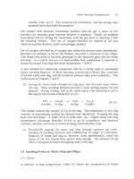
Comminution is performed in three stages:
(a) breaking the ore by explosions in the mine (blasting)
(b) crushing of large ore pieces by compression
in
eccentric crushers, Fig. 3.3
(c) wet grinding of the crushed ore in rotating ‘tumbling mills’
where
abrasion, impact and compression all contribute to breaking the ore, Fig.
3.4.
The final fineness of grind is mainly determined by the number of times an ore
particle passes through the grinding mills.
Separate crushing and grinding is necessary because it is not possible to break
massive run-of-mine ore pieces while at the same time controlling fineness of
grind for flotation.
34
Extractive Metallurgy
of
Copper
100
'%
recovery

=
100
x
mass
Cu
in concentratelmass
Cu
in ore
B
s
70:
60
103 74
52
37
Ore 26 particle size,
Pm
0.4
0.3
0.2
0.1
103 74
52
37
26
13
6
0.0
Ore particle size,
Pm

Fig.
3.2.
Effect of grind particle size on (a) copper recovery and
(b)
%
Cu
in
tailings.
The
presence
of
an optimum size
is
shown (Taggart,
1954).
%
recovery is calculated
from ore input rate (tonnedday),
%Cu
in
ore,
concentrate output rate (tonnedday) and
%
Cu
in concentrate.
3.2.2 Blasting
Blasting entails drilling holes in the minc, filling the holes with explosive and
exploding fragments
of
rock from the mine wall. The explosions send cracks

through the rock, releasing multiple fragments.
Fuerstenau
et
al.
(1997) report that closer drill holes and larger explosive charges
give smaller rock fragments. This may be useful for decreasing subsequent
crushing requirements.
Concentrating Copper Ores
35
3.2.3
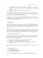
Crushing
Crushing is mostly done in the mine. This permits ore to be transported out of
an open-pit mine by conveyor. It is also permits easy hoisting of ore out of an
underground mine.
The crushed ore is stored in a coarse-ore stockpile from which it is sent by
conveyor to a semi-autogenous or autogenous grinding mill.
3.2.4
Grinding
Grinding takes the ore from crushing. It produces ore particles of sufficient
fineness for
Cu
mineral recovery by flotation. The most common grinding mills
are:
(a) semi-autogenous and autogenous mills
(b) ball mills.
Grinding is always done wet with mixtures of -80 mass% solids and
-20
mass%
water. A grinding circuit usually consists of one semi-autogenous or autogenous
mill

-
and one
or
two ball mills.
Grinding and subsequent flotation are continuous, connected operations.
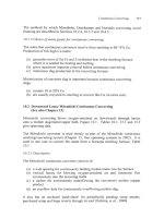
Autogenous mills tumble crushed ore without iron
or
steel grinding media.
They are used when the crushed ore pieces are hard enough to perform all the
grinding.
Semi-autogenous mills tumble mainly ore but they use -0.15 m3 of 13
cm iron or steel balls per
0.85
m3 of ore (Le. 15 volume% ‘steel’) to assist
grinding. Semi-autogenous mills are more common.
The semi-autogenous or autogenous mill grinds crusher product and prepares it
for final grinding in a ball mill. Its product is usually passed over a large
vibrating screen
to
separate oversize ‘pebbles’ from correct-size particles. The
correct-size material is sent forward to a ball mill for final grinding.
The
oversize pebbles are recycled through
a
small eccentric crusher, then back
to
the
semi-autogenous or autogenous mill. This procedure maximizes ore throughput
and minimizes electrical energy consumption.
Ball mills tumble iron

or
steel balls.
The balls are initially
5
to 10 cm diameter.
They gradually wear away as grinding proceeds. Ball mills typically contain
about
75%
ore and
25%
‘steel’ (by volume). They give a controlled final grind.
The ball mill accepts the semi-autogenous
or
autogenous mill product. It
produces uniform-size flotation feed.
It is operated in closed circuit with a
particle size measurement device and size control cyclones, Fig. 3.5. The
36
Extractive Metallurgy
of
Copper
ECCENTRIC DRIVE
3
Fig.
3.3. Gyratory crusher for crushing run-of-mine ore to
-20
cm pieces. The crushing
is done by compression of ore between the eccentrically rotating spindle and the fixed
crusher walls. The crushing surface on the spindle can be up to
3

m in height.
Fig.
3.4.
Semi-autogenous grinding mill. It
is
a rotating barrel in which ore
is
broken by
(i) itself and (ii) steel balls as they are lifted and fall off the moving circumference of the
barrel. Drawing courtesy www.bradken.com.au
Concentrating Copper Ores
37
Table
3.1.
Industrial crushing and grinding data
for
three copper concentrators, 2001.
They all treat ore from large open-pit mines. Flotation details are given in Table 3.3.
Concentrator
Candaleria, Chile Mexicana de Bagdad Copper,
Cobre, Mexico Arizona
Ore treated per year,
25
000
000
27 360
000
31
000
000

tonnes
Ore
grade, %Cu
Crushing
primary gyratory
crusher
diameter
x
height, m
power rating, kW
product
size,
m
energy consumption,
kWh per tonne of ore
secondary crushers
First
stage grinding
mill type
number
of
mills
diameter
x
length, m
power rating each
mill, kWh
rotation speed, RF'M
vol.
%

'steel' in mill
ball size, initial
ball consumption
feed
product size
oversize treatment
energy consumption,
kWh per tonne of
ore
Second stage grinding
mill type
number
of
mills
diameter
x
length, m
power rating each
mill, kW
rotation speed, RPM
vol.
%
'steel' in mill
feed
product size
energy consumption,
kWh per tonne of ore
Hydrocyclones
0.9
-

1.0
one
1.52
x
2.26
522
0.1-0.13
0.3
(estimate)
no
semi-autogenous
2
11
x
4.6
12
000
9.4-9.8
12-15
12.5 cm
0.3 kghonne ore
70%
ore,
80%
<
140
pm
22% ore recycle
through two 525
kW crushers

7.82
30%H20
ball mills
4
6x9
5600
0.522
2
1.52
x
2.26
375 at -600
RF'M
0.15
6
ball mills
12
5
x
7.3
4000
-13.8
32
80%
<2 15 pm
ball mills
4
4.3
x
7.3

-15
80% <58 pm
7
(estimate)
14
Krebs (0.5
m
diameter)
6
0.4
one
1.5
x
2.25
450
0.2
no
autogenous
5
10x4
4500
10
0
83%
ore
4
cm
screened and
recycled through
cone crushers

8
17%
H20
ball mills
5
4.7
x
6.7
2200
13
40
85% ore, 15%
H20
80%
<I30 pm
6
2 to
3
(0.85 m diameter)
Particle size monitor
Yes no
38
Extractive Metallurgy
of
Copper
cyclones send correct-size material
on
to flotation and oversize back to the ball
mill for further grinding.
3.3

Flotation Feed Particle Size
A
critical step in grinding
is
ensuring that the final particles from grinding are
fine enough for efficient flotation.
Coarser particles must be isolated and
returned for further grinding.
Size control is universally done by hydrocyclones, Fig.
3.5
(Krebs,
2002).
The
hydrocyclone makes use of the principle that, under the influence of a force
field, large ore particles in a water-ore mixture (pulp) tend to move faster than
small ore particles.
This principle is put into practice by pumping the grinding mill discharges into
hydrocyclones at high speed,
5
to
10
m per second. The pulp enters tangentially,
Fig.
3.5,
so
it is given a rotational motion inside the cyclone. This creates a
centrifugal force which accelerates ore particles towards the cyclone wall.
The water content of the pulp,
-60
mass% H20, is adjusted

so
that:
(a) the oversize particles are able to reach the wall, where they are dragged
out by water flow along the wall and through the apex of the cyclone, Fig.
3.5
(b) the correct (small) size particles do not have time to reach the wall before
they are carried with the main flow of pulp through the vortex finder.
The principal control parameter for the hydrocyclone is the water content of the
incoming pulp.
An
increase in the water content of the pulp gives less
hindered movement of particles. It thereby allows a greater fraction of the
input particles to reach the wall and pass through the apex. This increases
the fraction of particles being recycled for regrinding and ultimately to a
more finely ground final product.
A decrease in water content has the opposite effect.
3.3.
I
Instrumentation and control
Grinding circuits are extensively instrumented and closely controlled, Fig.
3.6,
Table
3.2.
The objectives of the control are to:
(a) produce particles of appropriate size for efficient flotation recovery of
Cu
minerals
(b)
produce these particles at a rapid rate
(c) produce these particles with a minimum consumption

of
energy.
Concentrating Copper Ores
39
i~
APEX
VALVE
L
I
Coarse
1
fraction
Fig.
3.5.
Cutaway view of hydrocyclone showing tangential input of water-ore particle
feed and separation into fine particle and coarse particle fractions. The cut between fine
particles and coarse particles
is
controlled by adjusting the water content of the feed
mixture, Section 3.3. Drawing from Boldt and Queneau, 1967 courtesy Inco Limited.
The most common control strategy is to:
(a) insist that the sizes of particles in the final grinding product are within
predetermined limits, as sensed by an on-stream particle size analyzer
(Outokumpu, 2002a)
(b) optimize production rate and energy consumption while maintaining this
correct-size.
Fig.
3.6
and the following describe one such control system.
40

Extractive
Metallurgy
of
Copper
a
Particle size
@c-&
H2°
control
loop
,
.
.

.
-
.
.
.

.
-
!
I
I
!
Crushed
I
Flotation feed
I

Mass
flow
control
loop
Fig.
3.6.
Control system for grinding mill circuit
(-
ore
flow;

water
flow;
electronic control signals). The circled symbols refer to the sensing
devices in Table
3.2.
A
circuit usually consists of a semi-autogenous grinding mill, a
hydrocyclone feed sump, a hydrocyclone 'pack'
(-6
cyclones) and one
or
two
ball mills.
(Screening and crushing
of
oversize semi-autogenous grinding mill pieces
is
not shown.)
3.3.2

Particle size control
The particle-size control loop in Fig.
3.6
controls the particle size of the grinding
product by automatically adjusting the rate of water addition to the hydrocyclone
feed sump. If, for example, the flotation feed contains too many large particles,
an electronic signal from the particle size analyzer
(S)
automatically activates
water valves to increase the water content of the hydrocyclone feed. This
increases the fraction of the ore being recycled to the ball mills and gives ajiner
grind.
Conversely, too fine a flotation feed automatically cuts back
on
the rate of water
addition to the hydrocyclone feed sump. This decreases ore recycle to the
grinding meals, increasing flotation feed particle size. It also permits a more
rapid initial feed to the ball mills
and
minimizes grinding energy consumption.
3.3.3
Ore throughput control
The second control loop in Fig.
3.6
gives maximum ore throughput rate without
overloading the ball mill. Overloading might become a problem if, for example,
Concentrating
Copper
Ores
4

I
the ball mill receives tough, large particles which require extensive grinding to
achieve the small particle size needed by flotation.
The simplest
mass
flow
control scheme is to use hydrocyclone sump pulp level
to
adjust ore feed rate to the grinding plant. If,
for
example, pulp level
sensor
(L)
detects that the pulp level
is
rising (due to tougher ore and
more
hydrocyclone recycle), it automatically
slows
the plant’s input ore feed
conveyor. This decreases
flow
rates throughout the plant and stabilizes ball mill
loading and sump level.
Detection
of
a
falling sump level, on the other hand, automatically increases ore
feed rate to the grinding plant
-

to
a
prescribed rate or to the maximum capacity
of
another part
of
the concentrator, e.g. flotation.
Table
3.2.
Sensing and control devices for grinding circuit shown in Fig.
3.6.
Use
in automatic
Type of device control system
Purpose
Sensing Symbol
instruments Firr.
3.6
Ore
tonnage
0
weight-
ometer
Water flow
gages
W
On-stream
size
analyzer
particle

S
Hydro-
cyclone
level
indicator
feed sump
L
Ball mill
load
Senses feed rate
of
ore into grinding conveyor speed
circuit
Load cells,
Sense water Rotameters
addition rates
Senses
a critical Measure
particle size ultrasound
parameter (e.g. energy
loss
in
percent minus
150
de-aerated pulp
pm)
on
the basis (Outokumpu,
of
calibration 2002a)

curves for the
specific ore
Senses changes
of
Bubble pressure
pulp level in tubes; electric
sump; triggers contact probes;
alarms for ultrasonic
impending over- echoes; nuclear
flow
beam
Senses mass of
ore
in ball mill sound, bearing
Load cells;
pressures; power
draw
Controls ore feed
rate
Control waterlore
ratio in grinding
mill
feed
Controls water
addition rate to
hydrocyclone feed
(which controls the
particle size
of
the

final grinding circuit
product)
Controls rate of ore
input into grinding
circuit (prevents
over-loading of ball
mills
or
hydro-
cyclones)
Controls rate of
ore
input into grinding
circuit