Kinetics of Materials - R. Balluff_ S. Allen_ W. Carter (Wiley_ 2005) Episode 4 doc

114
CHAPTER
5:
SOLUTIONS
TO THE
DIFFUSION EQUATION
An estimate of the penetration distance for the error-function solution (Eq. 5.23)
is the distance where
c(x,
t)
=
~0/8,
or equivalently, erf[x/(2m)]
=
-3/4: which
corresponds to
x
RZ
1.6fi
(5.71)
A reasonable estimate for the penetration depth is therefore again
2m.
To
estimate the time at which steady-state conditions are expected, the required
penetration distance is set equal to the largest characteristic length over which
diffusion can take place in the system. If
L
is the characteristic linear dimension
of a body, steady state may be expected to apply
at
times

r
>>
L2/Dmin,
where
Dmin
is the smallest value of the diffusivity in the body. Of course, there are many
physical situations where steady-state conditions will never arise, such as when the
boundary conditions are time dependent or the system is infinite or semi-infinite.
Bibliography
1.
P.M.
Morse and
H.
Feshbach.
Methods
of
Theoretical Physics,
Vols.
1
and
2.
McGraw-
2.
J.
Crank.
The Mathematics
of
Diffusion.
Oxford University Press, Oxford, 2nd edition,
3. H.S. Carslaw and

J.C. Jaeger.
Conduction
of
Heat in Solids.
Oxford University Press,
Hill, New York, 1953.
1975.
Oxford, 2nd edition, 1959.
EXERCISES
5.1
A
flat
bilayer slab is composed of layers of material
A
and
B,
each of thickness
L.
A component is diffusing through the bilayer in the steady state under
conditions where its concentration is maintained at
c
=
co
=
constant at one
surface and at
c
=
0
at the other. Its diffusivity

is
equal to the constants
DA
and
DB
in the two layers, respectively.
No
other components in the system
diffuse significantly.
Does the flux through the bilayer depend on whether the concentration is
maintained at
c
=
co
at the surface of the
A
layer or the surface of the
B
layer? Assume that the concentration of the diffusing component is continuous
at the
A/B
interface.
Solution.
Solve
for
the difFusion in each layer and match the solutions across the
A/B
interface. Assume that
c
=

co
at the surface of the
A
layer and let
c
=
c~/~
be the
concentration at the
A/B
interface. Using
Eq.
5.5,
the concentration in the
A
layer in
the interval
0
<
x
<
L
is
(5.72)
(5.73)
For
the
B
slab in the interval
L

5
x
5
2L,
(5.75)
EXERCISES
115
Setting
JA
=
JB
and solving for
cAIB,
DA
DA
+
DB
co
CAIB
=
The steady-state flux through the bilayer
is
then
c0
D~D~
J=-
L
DA+DB
(5.76)
(5.77)

J
is
invariant with respect to switching the materials in the two slabs, and therefore
it
does not matter on which surface
c
=
CO.
5.2 Find an expression for the steady-state concentration profile during the radial
diffusion of a diffusant through a cylindrical shell of thickness,
AR,
and inner
radius,
R'",
in which the diffusivity is a function of radius
D(r).
The boundary
conditions are
C(T
=
R'")
=
c'"
and
c(r
=
R'"
+
AR)
=

coUt.
Solution.
The gradient operator in cylindrical coordinates is
d
16
d
dr
rd0
dz
V
=
-Cr
+
go
+
-Cz
The divergence of a flux J'in cylindrical coordinates is
-
1
d(rJr)
1
dJ0 dJ,
V.
J=
+ +-
r dr
r
d0
dz
Therefore, the steady-state radially-symmetric difFusion equation becomes

which can be integrated twice to give
(5.78)
(5.79)
(5.80)
(5.81)
The integration constant
a1
is
determined by the boundary condition at
R'"
+
AR:
(5.82)
5.3
Find the steady-state concentration profile during the radial diffusion of a
diffusant through a bilayer cylindrical shell of inner radius,
R'",
where each
layer has thickness
AR/2
and the constant diffusivities in the inner and outer
layers are
Din
and
DOut.
The boundary conditions are
c(r
=
R'")
=

c'"
and
C(T
=
R'"
+
AR)
=
coUt.
Will the total diffusion current through the cylinder
be the same if the materials that make up the inner and outer shells are
exchanged? Assume that the concentration of the diffusant is the same in the
inner and outer layers at the bilayer interface.
Solution.
The concentration profile at the bilayer interface will not have continuous
derivatives. Break the problem into separate difFusion problems in each layer and then
impose the continuity of flux at the interface. Let the concentration at the bilayer
interface be
Inner region:
R'"
5
r
5
Ri"
+
116
CHAPTER
5.
SOLUTIONS
TO THE

DIFFUSION
EQUATION
Using Eq. 5.82,
The flux at the bilayer interface
is
Outer region:
R'"
+
5
r
5
Rin
+
AR
r
+
$0
C~ut
-
ci/o
R'"+AR
In
(
R1"+AR/2)
In
(
Rin
+
AR/2
COUt(T)

=
The flux at the bilayer interface is
Setting the fluxes at the interfaces equal and solving for
ci/O
yields
Cy~ut
out
+
ainCin
aout
+
Cyin
ci/o
=
c
where
R'"
+
A
R/
2
(5.83)
(5.84)
(5.85)
(5.86)
(5.87)
(5.88)
Putting Eq. 5.87 into Eqs. 5.83 and 5.85 yields the concentration profile of the entire
cylinder
.

The total current diffusing through the cylinder (per unit length)
is
Using Eq. 5.87,
aout
(Gout
-
Gin)
ci/o
-
-
-
@out
+
(5.89)
(5.90)
If
everything
is
kept constant except
Din
and
DOut,
use of Eq. 5.90 in Eq. 5.89 shows
that
nin
nout
uu
IK
CY~
DOut

+
CY~
Din
(5.91)
where
a1
and
a2
are constants. Clearly,
I
will be different
if
the materials making up the
inner and outer shells are exchanged and the values of
DOut
and
Din
are therefore ex-
changed. This contrasts with the result for the two adjoining flat slabs in Exercise 5.1.
5.4
Suppose that a very thin planar layer of radioactive Au tracer atoms is placed
between two bars of Au to produce a thin source of diffusant as illustrated
in Fig. 5.8. A diffusion anneal will cause the tracer atoms to spread by
self-diffusion as illustrated in Fig. 5.3.
(A mathematical treatment of this
spreading out is presented in Section 4.2.3.) Suppose that the diffusion ex-
EXERCISES
117
Thin source
Figure

5.8:
Thin planar tracer-atom source between two long bars.
periment is now carried out with
a
constant electric current passing through
the bars along
x.
(a)
Using the statement of Exercise
3.10,
describe the difference between the
way in which the tracer atoms spread out when the current is present
and when it is absent.
(b)
Assuming that
DVCV
is known, how could you use this experiment to
determine the electromigration parameter
p
for Au?
Solution.
(a) The electric current produces a flux of vacancies in one direction and an equal
flux of atoms in the reverse direction,
so
that
4
+
JA
=
-Jv

(5.92)
Using the statement of Exercise
3.10,
this will result in an average drift velocity
for each atom, given by
(5.93)
The tracer atoms will spread out as they would in the absence of current: however,
they will also be translated bodily by the distance
Ax
=
(VA)t
relative to an
embedded inert marker as illustrated in Fig.
5.9.
Inert
em bedded
marker
(a)
t=O
1
1
4
I
I
Figure
5.9:
(a)
The initially thin distribution of tracer atoms that, subsequently, will
spread due to diffusion and drift due to electromigration.
(b)

The electromigration has
caused the distribution to spread out and to be translated bodily by
Ax
=
(VA)t
relative to
the fixed marker.
118
CHAPTER
5:
SOLUTIONS
TO
THE
DIFFUSION
EQUATION
This may be shown by choosing an origin at the initial position of the source in
a coordinate system fixed with respect to the marker. The diffusion equation is
then
(5.94)
where
(VA)C
is the flux due to the drift. Defining a moving (primed) coordinate
system with its origin at
x
=
(‘UA)t,
2’
=
X
-

(WA)t
(5.95)
Using
[a(
)/ax],
=
[a(
)/ad]t,
the drift velocity does not appear in the resulting
diffusion equation in the primed coordinate system, which is
d
*c
*
a2
*c
at
ax‘2
-=
D-
The solution in this coordinate system can be obtained from Table 5.1;
nd
e-e’2/(4*Dt)
*c(x/,
t)
=
-
dm
(5.96)
(5.97)
The distribution therefore

spreads
independently of
(wA),
but is translated with
velocity
(VA)
with respect to the marker.
(b)
The velocity
(V)A
can be measured experimentally and then
p
can be obtained
through use of Eq. 5.93
if
DVCV
is known.
It
will be seen in Chapter
8
that
DVCV
can be determined by use of Eq.
8.17
if
*D
is known.
*D
can be determined from
the measured distribution illustrated in Fig. 5.96 using

Eq.
5.97 and the method
outlined in Section
5.2.1.
5.5
Obtain the instantaneous plane-source solution in Table
5.1
by representing
the plane source as an array
of
instantaneous point sources in a plane and
integrating the contributions
of
all the point sources.
Solution.
Assume an infinite plane containing
m
point sources per unit area each of
strength nd.
The plane
is
located in the
(y~)
plane
at
x
=
0.
All
the point sources

in the plane lying within a thin annular ring of radius
r
and thickness
dr
centered on
the z-axis will contribute a concentration at the point
P
located along the x-axis at a
distance, x, given by
nd
e-(z2+r2)/(4Dt)
(47rDt)3I2
dc
=
m27rr
dr
(5.98)
where the point-source solution in Table 5.1 has been used. The total concentration
is
then obtained by integrating over
all
the point sources in the plane,
so
that
where
M
=
mnd
is the total strength of the planar source per unit area.
5.6

Consider an infinite bar extending from
-cc
to
+cc
along
x.
Starting at
t
=
0,
heat is generated at a constant rate in the
x
=
0
plane. Show that the
temperature distribution along the bar is
(5.100)
EXERCISES
119
where
P
=
power input at
x
=
0
(per unit area) and
cp
=
specific heat per

unit volume. Next, show that
Finally, verify that this solution satisfies the conservation condition
x
T(z,
t)
cp
dx
=
Pt
Solution.
The amount of heat added (per unit area) at
z
=
0
in time
dt
is
Pdt.
Using the analogy between problems of mass diffusion and heat flow (Section
4.1),
each
added amount of heat,
Pdt,
spreads according to the one-dimensional solution for mass
diffusion from a planar source in Table
5.1:
dT=-[
1 Pdt
]
e-z2/(4nt)

CP
2(7rKt)1/2
(5.102)
Because the term in brackets represents an incremental energy input per unit volume, the
factor
(cp)-’
must be included to obtain an expression for the corresponding incremental
temperature rise,
dT.
Let
Then
2
X2
a2=lG
t=y-
P
a1
=
-
2CP
J
J:/”
exp
(-my2)
T(x,y)
=
-2a1
dY
Y2
(5.103)

(5.104)
Integrating by parts and converting back to the variables
(z,
t)
yields
~(z,
t)
=
2a1
e-azltd2
+
4a16
eCCZ
d<
(5.105)
Substituting for
a1
and
a2,
we finally obtain
(5.106)
Note that the solution given by Eq.
5.106
holds for
z
2
0
because the positive root of
&
was used. The symmetric solution for

z
5
0
is easily obtained by changing the sign
of
z.
All
the heat stored in the specimen at the time
t
is
represented by the integral
Q
=
2
[w
T(a,
t)
cp
dx
The first bracketed term in
Eq.
5.107
has the value
2Pt.
The second term can be
integrated by parts and has the value
Pt.
Therefore,
Q
=

2Pt
-
Pt
=
Pt
and the stored heat is equal to the heat generated during the time
t,
given by
Pt.
120
CHAPTER
5
SOLUTIONS
TO
THE DIFFUSION EQUATION
5.7
Consider the following boundary-value problem:
dC
-(z
=
4m,
t)
=
0
ax
0
Use the superposition method to find the time-dependent solution.
Show that when
26
>>

a,
the solution in (a) reduces to a standard in-
stantaneous planar-source solution in which the initial distribution given
by
Eq.
5.108
serves as the source.
0
Use the following expansions for small
E:
(5.109)
2E
2
erf(z
+
E)
=
erf(z)
+
-e-'
+
*
*.
e'
=
1
+E+
J;;
Solution.
(a) The concentration of diffusant located between

6
and
5
+
d<
in the initial dis-
tribution acts as a planar source of thickness,
d<,
and produces a concentration
increment at a distance,
2,
given by
(5.110)
The total concentration produced at
x
is then obtained by integrating over the
distribution. Therefore,
Using the relations
oe-u2
du
=
-
J;;
[erf(P)
-
erf(cu)]
(5.112)
2
The solution is
(5.113)

x+a
x-a
c(2,
t)
=%
2a
{
erf
(
-)
x
-
erf
(
T)
EXERCISES
121
(b) Expanding Eq. 5.114 for small values of
a/A
=
a/m
produces the result
c(x,t)
=
-
(5.115)
This is just the solution for a planar source of strength
nd
corresponding to the
content per unit area of the original distribution given by Eq. 5.108.

5.8
(a)
Find the solution
c(z,
y,
z,
t)
of the constant-D diffusion problem where
the initial concentration is uniform at
CO,
inside a cube of volume
u3
centered at the origin. The concentration is initially zero outside the
cube. Therefore,
if
1x1
5
4
and
Iy1
5
$
and
121
5
4
otherwise
c(z,
y,
z,

t
=
0)
=
and
c(z
=
fm,
y
=
fml
z
=
Am,
t)
=
0
(b)
Show that when
2m
>>
a,
the solution reduces to a standard instan-
taneous point-source solution in which the contents
of
the cube serve as
the point source. Use the erf(z
+
E)
expansion in

Eq.
5.109.
Solution.
(a) The method of superposition of point-source solutions can be applied to this
problem. Taking the number of particles in a volume
dV
=
dXdqdC
equal to
dN
=
co
dXdqdC
as
a
point source and integrating over all point sources in the
cube using the point-source solution in Table 5.1, the concentration at
x,
y,
z
is
c(x,
Yl
2,
t)
co
dX
dqdC
e-[(~-~)2+(y-q)2+(z-C)z]/(4Dt)
(5.116)

(4~Dt)~l~
The integral can be factored
J-a/2
'
J-a/z
The integrals all have similar forms. Consider the first one. Let
u
=
(x-x)/a;
then
122
CHAPTER
5:
SOLUTIONS TO THE DIFFUSION EQUATION
Therefore, the solution can be written
x
-
a/2
(b)
Expansion of Eq. 5.119 using Eq. 5.109 produces the result
cga3
-r2/(4Dt)
(47rDt)3/2
C=
(5.119)
which is just the solution for a point source containing the contents
of
the cube
corresponding to cga3 particles.
5.9

Determine the temperature distribution
T
=
T(z,
y,
2,
t)
produced by an ini-
tial point source of heat in an infinite graphite crystal. Plot isothermal curves
for a fixed temperature as a function of time in:
(a)
The basal plane containing the point source
(b)
A
plane containing the point source with a normal that makes a
60"
(c)
A
plane containing the c-axis and the point source
angle with the c-axis
The thermal diffusivity in the basal plane is isotropic and the diffusivity along
the c-axis is smaller than in the basal plane by a factor of
4.
Solution.
Using Eq. 4.61 and the analogy between mass diffusion and thermal diffusion,
the basic differential equation for the temperature distribution in graphite can be written
(5.120)
where
21
and

22
are the two principal coordinate axes in the basal plane and
23
is the
principal coordinate along the c-axis.
In order to make use of the point-source solution for an isotropic medium as in Sec-
tion 4.5, rescale the axes
Then Eq. 5.120 becomes
dT
at
-
=
(RiRL)
The solution
of
Eq. 5.122 for the point source in
(Table 5.1)
53
=
1/6
6
(5.121)
(qh)
(5.122)
these coordinates then has the form
T
-
e-(€:+Eg+E~)/[4(kini)1/3tl
(5.123)
t3/2

where
cy
is
a constant. Converting back to the principal axis coordinates yields
(5.124)
EXERCISES
123
(a)
Isotherms in the basal plane: In the basal plane passing through the origin,
3%
=
0
(5.125)
Q
and
T
22,
%3
=
0,
t)
=
-
,-(*?+*P)/(4kllt)
t3/2
Isotherms
for
a fixed temperature at increasing times are shown in Fig.
5.10.
They are circles,

as
expected, because the thermal conductivity is isotropic in the
basal plane. Initially, the isotherms spread out and expand because
of
the heat
conduction but they will eventually reverse themselves and contract toward the
origin, due to the finite nature of the initial point source of heat.
h
i
Figure
5.10:
passes through the origin.
Isotherms for
a
fixed temperature at increasing times in
a
basal plane that
(b) Isotherms in a
60"
inclined plane: The isotherms on a plane with a normal in-
clined
60"
with respect to the c-axis can be determined by expressing the solution
(Eq.
5.124)
in a new coordinate system rotated
60"
about the
21
axis. The new

(primed) coordinates are
0
( )
=
(
;os60" sin60'
)
(
ii
)
0
-sin60" cos60"
In the new coordinates, with
zb
=
0,
the temperature profile in the inclined plane
passing through the origin is
Figure
5.11
shows the isotherms as a function of time. Again the curves expand
and contract with increasing time. However, the isotherms are elliptical because
the thermal conductivity coefFicient is different along the c-axis and in the basal
plane.
124
CHAPTER 5:
SOLUTIONS
TO
THE
DIFFUSION

EQUATION
Figure
5.11:
normal inclined
60'
from the c-axis and passing through the origin.
Isotherms
for
a fixed temperature at increasing times in a plane with its
(c) Isotherms on
a
plane containing the c-axis: Here we simply examine the plane con-
taining
21
and
&.
The temperature profile on this plane
is
T(&,62
=0,23,t)
=
t3/2exp
cy
[-
(&+&)I
(5.127)
The isotherms are shown in Fig. 5.12. Again they expand and contract with
increasing time. The elliptical isotherms are slightly more eccentric than those in
Fig. 5.11 because
of

the greater rotation away from the basal plane.
Figure
5.12:
23
(the c-axis) and
21.
Isotherms
for
a
fixed temperature
at
increasing times in a plane containing
5.10
Consider one-dimensional diffusion in an infinite medium with a periodic
"square wave" initial condition given
by
if
0
5
2
+
n~
5
$
otherwise
c(2,t
=
0)
=
(5.128)

where
n
takes on all (positive and negative) integer values.
EXERCISES
125
(a)
Obtain a solution involving an infinite sine series.
(b)
Investigate the accuracy of truncating the full series solution. How many
sine terms must be retained in order for the concentration at
x
=
X/4
to agree with the full solution to within
1%
when
Dt/X2
=
0.002?
Solution.
(a) Use the method of separation of variables. Let
c(x,t)
=
Y(x)T(t).
Substituting
this into the diffusion equation yields
(5.129)
where
q
is a constant. The solutions to these two ordinary differential equations

a re
T
=
a1
exp(-qDt)
Y(x)
=
bl
sin(&x)
+
bzcos(&x)
(5.130)
where
al,
bl,
and
b2
are constants. The constant
b2
must be zero because the
initial concentration profile is an odd function
if
the origin
is
shifted upward by
-c0/2.
Further, the periodicity requires that
Y(&
(x
+

4)
=
Y(&X)
(5.131)
This condition will be satisfied
if
&A
=
27rm,
where
m
is an integer. Therefore,
solving for
q
and assigning it an index,
27rm
x
&=-
(5.132)
The general solution is then the sum of all the terms with different indices, plus a
constant,
Ao.
Thus,
(5.133)
The coefficients can be determined by using the initial condition given by Eq.
5.128.
When
t
=
0,

Eq.
5.37
is a standard Fourier series with coefFicients given by
2m7rx
x
x
A0
=
c(x,
0)
dx
A,
=
f
1
c(x,
0)
sin
(x>
dx
(5.134)
Inserting Eq.
5.128
and integrating,
A0
=
c0/2
and
A,
=

2co/(m7r)
for
m
odd
and
A,
=
0
for
m
even. Therefore,
(b) Symbolic algebra software can efFiciently calculate the partial sums in Eq.
5.135
for
the specified values of
x
and
Dt/X2.
Setting
co
=
1,
partial sums for
1
to
10
sine
terms give the values:
1.08829, 0.984021, 1.00171, 0.999809, 0.999927, 0.999923,
0.999923, 0.999923, 0.999923, 0.999923,

respectively. The series converges fairly
rapidly to a value of approximately
0.9999,
From the partial sums calculated,
three sine terms are required to give a concentration value that is within
1%
of
that given by the complete series. Note that successive terms in the sum are of
opposite sign, causing the partial sums to oscillate about the exact value of the
complete sum.
126
5.11
5.12
CHAPTER
5:
SOLUTIONS TO THE DIFFUSION EQUATION
Consider a plate of thickness
L
(0
<
x
<
L)
with the following boundary and
initial conditions:
T(x
=
0,
t)
=

0
T(x
=
L,t)
=
0
T(z,
t
=
0)
=
To
sin
Assume that the thermal diffusivity,
IE.,
is constant.
(a)
Find an exact expression for the temperature as a function of time.
(b)
Find an exact relation for
tlp,
the time when the temperature at the
(c)
If the heat flux at the surface of the plate is set to zero, would the time
center of the plate drops to
T0/2
(half its initial value).
calculated in part (b) be longer, shorter, or the same?
Solution.
(a) Use the separation-of-variables method as in Exercise

5.10.
Assume a solution of
the form
T(x,t)
=
Y(x)T(t).
Putting this into the thermal diffusion equation,
two ordinary difFerential equations are obtained whose solutions are
T(t)
=
a1
exp(-qnt)
Y(x)
=
bl
sin
(fix)
+
bz
cos
(fix)
(5.136)
where
al,
bl,
bz,
and
q
are constants. The resulting product solution can be fitted
to the initial and boundary conditions by setting

al
=
1,
bl
=
To,
bz
=
0,
and
fi
=
r/L,
so
that
T
=
T,
sin
(n:)
e-r’fitl~~
(5.137)
Equation
5.137
is a sine-series solution to the diffusion equation, but because of
the sinusoidal initial condition,
it
consists of only a single term.
(b) Setting
T

=
T0/2,
x
=
L/2,
and
t
=
tllz
in Eq.
5.137,
the time for the temper-
ature in the center of the plate to drop to half
its
initial value is
L2
tlp
=

ln(0.5)
7r2n
(5.138)
(c) Much longer! In fact,
if
no
heat
is
allowed to leave the plate, the fixed amount
of heat in the plate will spread until the temperature everywhere is uniform at the
value

T,
given by
2
T,
=
lL
To
sin
(rz)
dx
=
-To
r
(5.139)
The temperature in the center will therefore never drop to the level
T
=
T,/2!
It is desired to de-gas a thick plate of material containing a uniform concen-
tration of dissolved gas by annealing it in a vacuum. The rate at which the
gas leaves the plate surface is proportional to its concentration
at
the surface;
that is,
Jsurf
=
-a
csurf
(5.140)
where

a
=
constant.
(a)
Solve this diffusion problem during the early de-gassing period before
the outward diffusion of gas has any significant effect at the center of
EXERCISES
127
the plate. The initial and boundary conditions are therefore
c(z,O)
=
co
c(oo,~)
=
co
J=
-D
=
-a
~(0,
t)
(5.141)
Incorporate the parameter
h
=
a/D
into the solution.
(b)
Show that when the dimensionless parameter
ha

is large,
c(0,
t)
M
0,
and that when
ha
is small,
c(0,t)
M
co.
You will need the following
series expansions of erf(z):
For small
z,
(5.142)
and for large
z,
+ )
1
1
1x3 1X3X5
-
-
-
+
-
-
239
erfc(z)

=
1
-
erf(z)
=
(5.143)
(c)
Give a physical interpretation
of
the results in (b).
Solution.
(a) Use the Laplace transform method. Transforming the diffusion equation along
with the initial condition given by Eq. 5.141 yields the same result as Eq. 5.64:
The solution is therefore Eq. 5.65 with
a1
=
0:
co
P
~(x,p)
=
-
+
u2
e-mm
(5.144)
(5.145)
To
determine
u2,

transform the boundary condition given by Eq. 5.141 to obtain
-D
(g)
=
-a
E(0,p)
x=o
Therefore, putting Eq. 5.145 into Eq. 5.146 yields
CY
Cn
and
(5.146)
(5.147)
(5.148)
where
h
=
a/D.
Find the desired solution by taking the inverse transform using
a table of transforms to obtain
X
c(x,
t)
=
co
[erf
(
m)
+
eh=+h2gt

erfc
(&
+
hm)]
(5.149)
(b) From Eq. 5.149 the concentration at the surface is
c(0,
t)
=
co
e-h2’(Dt)
erfc
(hm)
(5.150)
128
CHAPTER
5:
SOLUTIONS
TO
THE
DIFFUSION
EQUATION
For large
hm,
use the series expansion for
a
large argument, to obtain
co
c(0,
t)

=
-
ha
(5.151)
Therefore,
c(0,t)
approaches zero for large hm. For small hm, use the
small-argument expansion to obtain
~(0,
t)
=
co
(1
+
h2Dt)
(5.152)
Therefore,
c(0,
t)
approaches
co
for small
hm,
(c) We can rewrite
hm
as
am.
Therefore, as
cy
becomes small, or at short

times
t,
or as
D
increases,
c(0,
t)
approaches
CO.
For small
a,
surface desorption
is compensated by diffusion from the bulk,
so
that
c(0,
t)
decreases slowly. How-
ever, at short times, the concentration gradients near the surface will be large,
so
c(0,
t)
will initially change rapidly. With large D, bulk difFusion to the surface
compensates the surface desorption. The reverse applies for large values of
hfi.
5.13
Solve the following boundary value problem on the semi-infinite domain with
discontinuous initial conditions,
co O<x<L
{

0
L<x<m
c(x,
t
=
0)
=
with zero flux conditions at
x
=
0
and
x
=
cm.
Suggestion:
Use superposition
of
known solutions, or split the problem into
two parts and use continuity to match Laplace-transformed solutions.
Solution.
Designate the region
z
<
L
as region
I
and the region
x
>

L
as
region
II.
The Laplace transform method will be used to solve the problem in each region
and the solutions will then be matched across the interface at
z
=
L.
In region
I
the diffusion equation and initial condition are the same as in the problem leading to
Eq. 5.64, and therefore the general solution after Laplace transforming corresponds to
Eq. 5.65. Similarly, in region
11,
the initial condition is the same as in the problem
leading to Eq. 5.58 and the general solution therefore corresponds to Eq. 5.59. The
four constants
of
integration can be determined from the boundary conditions imposed
at
z
=
0,
z
=
L,
and
z
=

co.
After Laplace transforming, these become
(5.153)
(5.154)
E'(L,p)
=
EJ'(L,p)
(5.155)
After determining the four constants of integration and putting them into Eqs. 5.59
and 5.65, the solutions in regions
I
and
II
are
I
co
co
E
=
-
-
-
exp(-ql) [exp(qz)
+
exp(-qz)]
(5.156)
P 2P
co
6''
=

exp(-qz) [exp(-qL)
-
exp(q~)l
2P
EXERCISES
129
where
q
=
@,
Using standard tables of transforms to transform back to
(2,
t)
coordinates, the final solutions are
Because erf(z)
=
-erf(-z), the solutions are identical in the two regions and thus
c(x,
t)
=
2
2
[erf
(s)
-
erf
(%)I
(5.158)
CHAPTER

6
DIFFUSION IN MU
LTICOM
PON ENT
SYSTEMS
In earlier chapters we examined systems with one or two types of diffusing chem-
ical species. For binary solutions, a single interdiffusivity,
5,
suffices to describe
composition evolution.
In
this chapter we treat diffusion in ternary and larger mul-
ticomponent systems that have two or more independent composition variables.
Analysis of such diffusion is complex because multiple cross terms and particle-
particle chemical interaction terms appear. The cross terms result in
N2
indepen-
dent interdiffusivities for a solution with
N
independent components. The increased
complexity
of
multicomponent diffusion produces a wide variety
of
diffusional phe-
nomena.
The general treatment for multicomponent diffusion results in linear systems
of diffusion equations. A linear transformation of the concentrations produces a
simplified system of uncoupled linear diffusion equations for which general solutions
can be obtained by methods presented in Chapter

5.
6.1
GENERAL FORMULATION
In Chapter
2
we considered diffusion in a closed system containing
N
components,
exclusive of any mediating point defects.l
If
only chemical potential gradients are
present and all other driving forces-such as thermal gradients or electric fields-
'Such defects,
if
present, will be assumed to be in local thermal equilibrium at very small concen-
trations.
Kinetics
of
Materials.
By
Robert W. Balluffi, Samuel
M.
Allen, and W. Craig Carter.
131
Copyright
@
2005 John Wiley
&
Sons, Inc.
132

CHAPTER
6
DIFFUSION IN
MULTICOMPONENT SYSTEMS
are absent, the general formulation presented in Eq.
2.21
and developed further in
Chapter 3 applies, and for one-dimensional diffusion,’
Equation 2.15 for the rate of entropy production is then
Assuming that the atomic volumes of the components are constants and the fluxes
are measured in a V-frame,
as
defined in Section 3.1.3, Eq. 3.22 holds for all
N
components,
N
CQiJi
=
0
i=l
The Nth flux can now be eliminated in Eq. 6.2 by using Eq. 6.3 and putting the
result into Eq. 6.2, so that
.(
N-1
and
The force,
Fi,
conjugate to the flux,
Ji,
is

and therefore the general linear relation between the independent fluxes and the
N
-
1
independent driving forces is
The chemical potential gradients and Onsager coefficients in Eq. 6.7 can be con-
verted to concentration gradients and interdiffusivities (Table
3.1).
Each chemical
potential in Eq. 6.7 is a function
of
the local concentration:
2This treatment is similar
to
that
of
Kirkaldy
and Young
[l].
6.1:
GENERAL FORMULATION
133
There are
N
-
1
independent concentrations because Eq. A.10 provides a single
relation between concentrations and their atomic volumes.
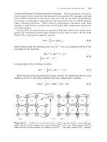
Under the assumption of local equilibrium, the Gibbs-Duhem relation applies,
which places an additional constraint on chemical potential changes in Eq. 6.7 and

implies that only
N
-
1
of
the
pi
can vary independently:
Interdiffusivities,
Eij,
are defined by Eq. 6.10,
Dij
is the product of two matrices,
(6.9)
(6.10)
(6.11)
(6.12)
(6.13)
where the
Lik
are Onsager coefficients and
Tkj
are thermodynamic factors that
couple chemical potentials to concentrations,
(6.14)
The analysis of
concentrations and
the diffusion for
N
components requires

N
-
1
independent
(N
-
1)2
interdiffusivities. For the ternary case,
(6.15)
L
J
The eigenvalues,
Ah,
of the interdiffusivity matrix (see Eq. 4.62) must be real and
positive
[l].
For the ternary case,
where
134
CHAPTER
6
DIFFUSION IN MULTICOMPONENT SYSTEMS
The real and positive condition on the eigenvalues places physical limits on the
interdiffusivities. For the ternary case,
(6.18)
(511522
-
512521)
L
0

I I
The sum
(Dll
+
D22)
must be positive, but a direct interdiffusivity,
oii,
could be
negative and still satisfy the conditions in Eq. 6.18. The off-diagonal terms,
Eij,
need not be symmetric with respect to the exchange of
i
and
j.
In the steps leading to Eq. 6.5, the choice of the Nth component is arbitrary, and
a different set of values for the four interdiffusivities will be obtained for each choice.
However, each set leads to the same physical behavior predicted for the system: the
diffusion profiles
of
the three components predicted by the equations are indepen-
dent of the choice for N.3 For some choices, the interpretation of interdiffusivities
in terms of kinetic and thermodynamic data may be more straightforward
[l].
6.2
SOLUTIONS OF MULTICOMPONENT DIFFUSION EQUATIONS
Generally, a set of coupled diffusion equations arises for multiple-component diffu-
sion when
N
2
3.

The least complicated case is for ternary
(N
=
3)
systems that
have two independent concentrations (or fluxes) and a
2
x
2
matrix of interdiffusivi-
ties.
A
matrix and vector notation simplifies the general case. Below, the equations
are developed for the ternary case along with
a
parallel development using compact
notation for the more extended general case. Many characteristic features of gen-
eral multicomponent diffusion can be illustrated through specific solutions of the
ternary case.
The coupled ternary diffusion equations in one dimension are obtained from the
accumulation fluxes in Eq. 6.11:
_-
dCl
V.J1=-
+a
ax
(Ell%)
+
&
(E12$)

_-
ac2
-
-V.
J2
+a
=
-
(&%)
+
(5222)
(6.19)
at
at
dX
or
and generally,
-
ac'
=
-
a
[5E]
at
ax
-ax
(6.20)
(6.21)
In general, the
5ij

are functions
of
the concentrations,
so
these equations are
nonlinear. Numerical methods must then be employed. However, solutions can be
obtained for a variety of special cases, several of which are described below.
3This independence is similar to
a
constrained system's insensitivity to the choice
of
Nc
in Sec-
tion
2.2.2.
6.2:
SOLVING
THE DIFFUSION EQUATIONS
135
6.2.1
Constant
Diffusivities
If the interdiffusivities are each constant and uniform, the coupled ternary diffusion
equations, Eq. 6.20, are a linear system,
(6.22)
and in general,
=
5,Vzc'
(6.23)
It is possible to uncouple the expressions for the fluxes by diagonalizing the diffu-

sivity matrix through
a
coordinate transformation. The transformed interdiffusivity
matrix will have eigenvalues
Xi
as its diagonal entries. For the ternary system, the
eigenvalues are the
A&
from Eq. 6.16. There will be
N
positive eigenvalues
AN
in
the general case, where
N
is the number of indeKendent components.
According to E% 1.36, the eigenvectors
2i
of
D
form the columns of the matrix
that diagonalizes
12
by the coordinate transformation. For the ternary system, let
the eigenvector for the
(fast)
A+
eigenvalue be fand for the (slow)
A-
be

s':
dc'
at
-
-
The slow and fast eigendirections are related by an angle
8,
-
(6.25)
s'.
f
D2l
-
512
case
=
=
=
-
Iqlfl
J(Dll
-
zj22)2
+
(zj12
+
fj21)2
The transformation matrix,
A,
that diagonalizes

5
has columns formed by the
eigenvectors fand
3.
For the ternary case,
and for the general case,
and therefore
Transforming Eq. 6.43 yields
or
[;I=-[
;+]v[
:,I
(6.28)
(6.29)
(6.30)
136
CHAPTER
6:
DIFFUSION IN MULTICOMPONENT SYSTEMS
or
J,
=
-
X-VC,
Jp
=
-
X+Vcp
(6.31)
and the fluxes are seen to be uncoupled in the diagonalized system.

J,
and
Jp
are
the two fluxes in the diagonalized system given by
[$I=”-“
;;I
and
c,
and
cp
are the two concentrations given by
[
;;
]
=
A-l[
;;
]
These quantities therefore have the forms
J2
Dii
-
D22
+
A
2A
Ji
+
-021

J,
=
-
A
D2
1
Jp
=
-
J1
-
A
52
Dll-
D22
-
A
2A
and
-021
Dll-
D22
+A
c2
c1
+
2A
c,
=
-

A
Dll
-
D22
-
A
2A
c2
D2
1
cp
=-c1
-
A
(6.32)
(6.33)
(6.34)
(6.35)
The flux problem can now be easily solved in the diagonalized system using
Eq. 6.31; the solution can then be transformed back to the original concentration
coordinates by using the inverse relationships
and
[;:]=A[
:]
[:;I=”[
:;]
Steady-State Solutions.
For the steady-state case, Eq. 6.22 becomes
and in general,
If

has an inverse,
0’
=
kv2z
I- I-
-
D
O=Q
QV2Z
or
[
;]=v2[
:;]
(6.36)
(6.37)
(6.38)
(6.39)
(6.40)
(6.41)
6.2:
SOLVING
THE
DIFFUSION
EQUATIONS
137
that is,
v2ci
=
0
(6.42)

Therefore, Laplace's equation holds for each component separately. However, the
steady-state fluxes are interdependent, as may be seen from Eq. 6.11 for the ternary
case,
(6.43)
Time-Dependent Solutions.
In the time-dependent case, the diffusion equations
given by Eq. 6.23 are coupled. However, they can be uncoupled by again using the
diagonalizat ion met hod.
Using the transformation matrix
A
on Eq. 6.23 gives for the ternary case,
a
-[
at
cg
'.I
=[
;-
:+Iv2[
:;
]
and for the general case,
a
at
-
A1
0.'' 0 0
0x20:
:
0

.*.
0
0

0
AN-1
(6.44)
(6.45)
where the concentrations
Ei
are linear combinations given by the eigensystem trans-
formation of the actual components
ci.
Each partial-differential equation in the diagonal frame is independent:
Tr(@
-
A
at
In general,
(6.46)
(6.47)
138
CHAPTER
6:
DIFFUSION IN MULTICOMPONENT SYSTEMS
For one-dimensional ternary diffusion, the boundary and initial conditions-
c1(z
=
L,t),
c1(x

=
R,t),
cl(x,t
=
0),
c2(x
=
L,t),
CZ(X
=
R,t),
and
cz(x,t
=
0)-
become
I
-
c2(2,
t
=
0)
-021
A
Dii
-
522
+
A
2A

ca(s,t
=
0)
=
-
Cl(X,
t
=
0)
+
In general,
Z(x
=
L,
t)
=
A-lc'(x
=
L,
t)
qx,
t
=
0)
=
A-lc'(z,
t
=
0)
Z(x

=
R,
t)
=
A-lc'(x
=
R,
t)
+
(6.48)
(6.49)
The system is reduced to a set of uncoupled diffusion equations with diffusivities
constructed from the component interdiffusivities by a prescribed algorithm. Each
equation can be solved by methods described in Chapter
5.
The transient behavior
at
the interface of two ternary alloy compositions in a
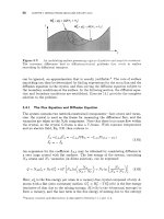
system with complete solid solubility will lead to a path in composition "space" as
shown in Fig.
6.1.
Evolution is initially parallel to the fast eigendirection Sand,
after its gradients become small, finally proceeds parallel to the slow direction
S:
+
c.
c
S
Figure
6.1:

specified
by
a
concentration pair on the left
(z
=
L)
and on the right
(z
=
R).
General evolution
of
a ternary diffusion couple with initial conditions
6.2.
SOLVING
THE
DIFFUSION
EQUATIONS
139
The solution for a diffusion couple in which two semi-infinite ternary alloys are
bonded initially at a planar interface is worked out in Exercise 6.1 by the same basic
method. Because each component has step-function initial conditions, the solution
is
a
sum of error-function solutions (see Section 4.2.2). Such diffusion couples are
used widely in experimental studies of ternary diffusion. In Fig. 6.2 the diffusion
profiles of Ni and Co are shown for a ternary diffusion couple fabricated by bonding
together two Fe-Ni-Co alloys of differing compositions. The Ni, which was initially
uniform throughout the couple, develops transient concentration gradients. This

example of uphill diffusion results from interactions with the other components in
the alloy. Coupling of the concentration profiles during diffusion in this ternary
case illustrates the complexities that are present in multicomponent diffusion but
absent from the binary case.
80
70
60
50
40
30
20
10
0
Distance (arbitrary scale)
Fi
ure
6.2:
wifi
Fe-Ni-Co alloys. From
Kirkaldy and
Young
[l],
and
Vignes
and Sabatier
[2].
Concentration profiles
for
Ni and
Co

in ternary diffusion couple fabricated
The results of ternary diffusion experiments are often presented in the form of
daflusion
paths,
which are plots of the concentrations measured across the diffusion
zone. The diffusion path corresponding to the measurements in Fig. 6.2 is shown
in Fig. 6.3; note the characteristic S-shape, due to the inflections in the
CN~
profile.
6.2.2
Concentration-Dependent Diffusivities
If the diffusivities are functions of concentration, the Boltzmann-Matano method,
described in Section 4.3 for the binary case, can be employed if the initial and
boundary conditions are appropriate. The diffusion equations are
(6.50)
and when the scaling parameter
77
=
x/d
is employed, these equations become
(6.51)