Kinetics of Materials - R. Balluff_ S. Allen_ W. Carter (Wiley_ 2005) Episode 11 doc

436
CHAPTER
18:
SPINODAL AND ORDER-DISORDER TRANSFORMATIONS
order parameters, such as for A2
-+
B2*
((qeq
=
0)
-+
(q
=
kqeq)),
there is no
bias to form one ordered
B2
variant over another (the two equivalent variants are
indicated by
B2*;
see Fig. 17.4). The two equivalent variants emerge
at
random
locations, and interfaces develop
as
one impinges upon the other. For conserved
order parameters, such
as
composition, interfaces between phases on phase-diagram
tie-lines necessarily appear.
In the absence of interfaces, a linear kinetic theory could be developed where

the transformation driving force derives from decreases in homogeneous molar free
energy
as
derived in Eqs. 17.28 and 17.29 for the conserved and nonconserved cases.
However, at the onset of a continuous phase transition, the system is virtually
all
interface between new phases or variants. For example, when equivalent variants
emerge in adjacent regions during ordering, gradients in the order parameter are
generated; these constitute emerging diffuse antiphase boundaries. Neglecting the
contribution of these interfaces leads to ill-posed linearized kinetics, as indicated
by the negative interdiffusivity in Eq. 18.9.
The theory for the free energy of inhomogeneous systems incorporates contribu-
tions from interfacial free energy through the
diffuse interface method
[3].
Interfaces
are defined by the locations where order parameters change and can be located by
the regions with significant order-parameter gradients. Interfacial energy appears
in the diffuse-interface methods because order-parameter gradients contribute extra
energy.
18.2.1
Let
J(F)
represent either a conserved or a nonconserved order parameter, such
as
CB(F)
or q(F). Also, let the field
f(F)
=
f(J(F),VJ(F))

be the free-energy density
(energy/volume) at position
F.
The homogeneous free-energy density,
f
=
f
(J,
VJ
=
0),
is the free-energy density in the absence of gradients and is related to
molar free energies,
F(J)
=
N,(R)
fhom(J),
used to construct phase diagrams such
as Figs. 17.5 and 17.7. Expanding the free-energy density about its homogeneous
value in powers of
gradient^,^
Free Energy
of
an inhomogeneous System
f
(e,
VC)
=
f(J,
0)

+
2
*
VJ
+
VJ
.
K
VJ
+
.
.
.
(18.10)
where
(18.11)
is a vector evaluated
at
zero gradient, and
K
is a tensor property known as the
gradient-energy coefficient with components
(18.12)
The free-energy density should not depend on the choice of coordinate system [i.e.,
f
(J,
05)
should not depend on the gradient's direction] and therefore
2
=

0
and
K
will be a symmetric ten~or.~ Furthermore, if the homogeneous material is isotropic
4There are expansions that contain higher-order spatial derivatives, but the resulting free energy
is the same
as
that derived here
[I,
41.
51f the homogeneous material has an inversion center (center
of
symmetry),
2
is automatically
zero.
18.2:
DIFFUSE INTERFACE THEORY
437
or
cubic,
K
will be a diagonal tensor with equal components K. The free-energy
density will be, to second order,
f
(E,
VE)
=
fhO"(E)
+

KVE
'
VE
=
fhO"(E)
+
KIVEI2
(18.13)
The free-energy density is thus approximated as the first two terms in a series
expansion in order-parameter gradients: the first term is related to homogeneous
molar free energy and the second is proportional to the gradient squared.
In the expansion that leads to Eq.
18.13,
it is assumed that the free energy varies
smoothly from its homogeneous value
as
the magnitude of the order-parameter
gradient increases from zero. This assumption is usually correct, but there may
be cases that include a lower-order term proportional to
lVSl
if the free-energy
density has a
cusp
at zero gradient. Such cusps appear in the interfacial free
energy at
a
faceting orientation; they are also present at small tilt-misorientation
grain-boundary energies
[5],
Models with crystallographic orientation as an order

parameter incorporate gradient magnitudes,
lV(l,
into the inhomogeneous free-
energy density
[6].
18.2.2
There are two energetic contributions to interfaces in systems that undergo decom-
position and ordering transformations such as illustrated in Figs.
17.5
and
17.7.
One is due to the gradient-energy term in Eq.
18.13;
this contribution tends to
spread the interface region and thereby reduce the gradient as the order parameter
changes between its stable values in adjacent phases.
A
second contribution derives
from the increased homogeneous free-energy density associated with the "hump"
in Fig.
18.1,
and this term tends to narrow the interface region. Thus, systems
modeled with Eq.
18.13
contain
diffuse interfaces
where the order parameter varies
smoothly as in Fig.
18.2.
Equilibrium order-parameter profiles and energies can be

determined by minimizing
F,
the volume integral of Eq.
18.13
[l,
41.
Figure
18.2a
shows a planar interface between two equilibrium phases possessing
different conserved order parameters corresponding to local free-energy density min-
ima in their order parameters
as
in Fig.
17.7a.
Figure
18.2b
shows a corresponding
profile of the distribution of order between two identical ordered domains possessing
different nonconserved order parameters corresponding to local free-energy density
Structure and Energy of Diffuse Interfaces
Ii
I
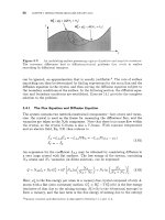
Figure
18.1:
which
has
the maximum value
A
f,!,;:.
Properties

of
diffuse interfaces expressed
in
ternis
of
the function
Afho"(<),
438
CHAPTER
18
SPINODAL AND ORDERDISORDER TRANSFORMATIONS
Figure
18.2:
(a)
Composition and
(b)
order variations across diffuse. planar interfaces.
The profiles
c(z)
and
q(z)
are continuous. In
(a).
the grayscale image represents the spatial
variation
of
a
conserved variable, and the quantities
ca'
and

ca"
are the equilibrium values
in the bulk phases
at
large distances from the interface (see Fig.
17.7).
In (b). the drawing
below the profile illustrates the spatial variation of a nonconserved variable such
as
local
magnetization in the region around
a
domain wall.
minima. Both kinds
of
interfaces can coexist,
so
that the variations of
CB
and
77
are coupled
as
in Fig.
18.3.
In
all
cases, the distribution of the order parameter
(or
order parameters) minimizes the total free energy

of
the system.
F.
The coupled-
parameter case can be treated
as
an extension to the theory
so
that the free energy
is
a
function
of
both
CE
and
17.
t
'I
or
c
X-
C
Figure
18.3:
antiphase boundary with segregation.
Coupled
system
of
order and concentration parameters representing

mi
18.2:
DIFFUSE INTERFACE THEORY
439
Minimizing
3
=
f
(<,
VE)dV
produces equilibrium interface profiles
[(q.
An
equilibrated planar interface
is
characterized by
its
excess energy per unit area,
y,
,=2l:
,/-,d[=
,/=A[
(18.14)
and a characteristic width
6,
(18.15)
where
A
fhom
is the increase in free-energy density relative to a homogeneous system

at its equilibrium values of
E
(i.e., relative to the common-tangent line) and
AfgT
is the maximum value of
Afhom
(indicated in Fig. 18.1).
y
and
6
can be measured
and their values uniquely determine the model parameters,
AfzT
and
K.
18.2.3
Diffusion Potential for Transformation
The local diffusion potential for a transformation,
@(q,
at a time t
=
to,
can be
determined from the rate of change of total free energy,
3,
with respect to its
current order-parameter field,
[(F,
to).
At time t

=
to,
the total free energy is
3(to)
=
s,
[fhom(C(F,
to))
+
KV5
.V5]
dV
(18.16)
which defines
3
as a functional of
[(F‘,
to).s
If the order parameter is changing with
local “velocity” [i.e., such that
[(F,
t)
=
c(F,
to)
+
((7,
to)t],
the rate of change
of

F
can be summed from all the contributions to
f([,
V[)
due to changes in the
order-parameter field and its gradient,
Using the relation
Eq. 18.17 can be written
(
18.17)
(18.18)
Applying the divergence theorem to the second integral in Eq. 18.19,
(18.20)
d3
itO
=
s,
(
:;(‘)
-
2KV2[)
4
dV
+
2K
1,
iV[
d2
where
aV

is the oriented surface bounding the volume
V.
The boundary integral on
the right-hand side of Eq. 18.20 is negligible. It vanishes identically if
i(8V)
=
0,
‘Some readers will recognize this development
as
the calculus of variations
[7].
A
functional
is
a
function of
a
function; in this case,
F
takes the function
[(F,
to)
and maps it to
a
scalar value
that is numerically equal
to
the total free energy of the system.
440
CHAPTER

18
SPINODAL
AND
ORDER-DISORDER TRANSFORMATIONS
which is the case if
[(dV)
has fixed boundary values (Dirichlet boundary condi-
tions), or if the projections of the gradients onto the boundary vanish (Neumann
boundary conditions), If neither Dirichlet or Neumann conditions apply, the bound-
ary integral will usually be insignificant compared to the volume integral for large
systems (e.g., if the volume-to-surface ratio is greater than any intrinsic length
scale).
Therefore, if the order parameter changes by a small amount
6[
=
(dt,
the
change in total free energy is the sum of local changes:
The quantity
(18.2
1)
(18.22)
is the localized density of free-energy change due to a variation in the order-
parameter field,
6[,
and is therefore the potential to change
[.
Equation 18.22
is the starting point for the development of kinetic equations for conserved and
nonconserved order-parameter fields.

18.3
EVOLUTION EQUATIONS FOR CONSERVED AND
NON-CONSERVED ORDER PARAMETERS
18.3.1 Cahn-Hilliard Equation
The Cahn-Hilliard equation applies to conserved order-parameter kinetics. For the
binary
A-B
alloy treated in Section
18.1,
the quantity in Eq. 18.22 is the change
in homogeneous and gradient energy due to a change of the local concentration
CB
and is related to
flux
by
(18.23)
where the subscript is affixed to the gradient energy coefficient
as
a reminder that
the homogeneous system is expanded in composition and its gradient.
Therefore, the accumulation gives a kinetic equation for the concentration
CB
(T,
t)
in an
A-B
alloy:
2KCV2c~]}
(18.24)
18.3:

EVOLUTION EQUATIONS FOR ORDER PARAMETERS
441
which is the Cahn-Hilliard equation
[3].
The Cahn-Hilliard equation is often lin-
earized for concentration around the average value of the inherently positive kinetic
coefficient
M,
=
(M)
=
(5/[0(a2Pom
)/(ax;)]),
defined in Eq. 18.9:
1
2
horn
~
dCB
=
Ado
[
~V'CB
-
2K,V4c~
at
(18.25)
The first term on the right-hand side in Eq. 18.25 is diffusive. The second term
accounts for interfacial-energy penalties from concentration gradients.
18.3.2 Allen-Cahn Equation

The Allen-Cahn equation applies to the kinetics of a diffuse-interface model for a
nonconserved order parameter-for example, the order-disorder parameter
~(7,
t)
that characterizes the A2
t
B2'
phase transformation treated in Section 17.1.2.
The increase in local free-energy density,
@(F)
from Eq. 18.22, does not require any
macroscopic flux.7 In a linear model, the local rate of change is proportional to its
energy-density decrease,
(18.26)
where
Mq
is a positive kinetic coefficient related to the microscopic rearrangement
kinetics. According to the Allen-Cahn equation, Eq. 18.26,
77
will be attracted to
the local minima of
fhorn.
Depending on initial variations in
77,
a system may seek
out multiple minima at a rate controlled by
Mq.
The second term on the right-hand
side in Eq. 18.26 will govern the profile of
77

at the antiphase boundary and will
cause interfaces to move toward their centers of curvature [8].
18.3.3
Numerical models of conserved order-parameter evolution and of nonconserved
order-parameter evolution produce simulations that capture many aspects of ob-
served microstructural evolution. These equations, as derived from variational prin-
ciples, constitute the phase-field method [9]. The phase-field method depends on
models for the homogeneous free-energy density for one or more order parameters,
kinetic assumptions for each order-parameter field (i.e., conserved order parameters
leading to a Cahn-Hilliard kinetic equation), model parameters for the gradient-
energy coefficients, subsidiary equations for any other fields such
as
heat flow, and
trustworthy numerical implementation.
The phase-field simulations reproduce
a
wide range of microstructural phenom-
ena such as dendrite formation in supercooled fixed-stoichiometry systems
[lo],
dendrite formation and segregation patterns in constitutionally supercooled alloy
systems
[ll],
elastic interactions between precipitates
[12],
and polycrystalline
so-
lidification, impingement, and grain growth [6].
Numerical Simulation and the Phase-Field Method
'This ordering transition occurs at constant composition and is accomplished by microscopic
re-arrangement

of
atoms into two sublattices.
442
CHAPTER
18:
SPINODAL
AND
ORDER-DISORDER
TRANSFORMATIONS
The simple two-dimensional phase-field simulations in Figs.
18.4
and
18.5
were
obtained by numerically solving the Cahn-Hilliard (Eq.
18.25)
and the Allen-Cahn
equations (Eq.
18.26).
Each simulation’s initial conditions consisted of unstable
order-parameter values from the “top of the hump” in Fig.
18.1
with a small spatial
Figure
18.4:
Example of numerical solution for the Cahn-Hilliard equation, Eq.
18.25.
demonstrating the kinetics
of
spinodal decomposition. The system is initially near

an unstable concentration,
(a),
and initially decomposes into two distinct phases with
compositions
ca
(black) and
cB
(white) with a characteristic length scale,
(c)
and
(d).
Subsequent evolution coarsens the length scale while maintaining fixed phase fractions. The
effective time interval between images increases from
(a)-(f).
Figure
18.5:
Example
of
numerical solution
for
the Allen-Cahn equation, Eq.
18.26,
for
an order-disorder transition such as
A2
+
B2*.
Initial data are near the disordered state.
7
=

0
(gray) in
(a).
The system evolves into two types of domains (shown in black and white)
with antiphase boundaries
(APBs)
separating them. The phase fractions are not fixed. The
local rate of antiphase boundary migration is proportional to interface curvature
[8.
131.
The
effective time interval between images increases from
(a)-(f).
18.4:
DECOMPOSITION AND ORDER-DISORDER: INITIAL STAGES
443
variation. In each simulation, the magnitude of the order parameter is indicated by
grayscale. Initial medium gray values correspond to the unstable initial conditions.
The characteristics of the initial evolution during spinodal decomposition or
order-disorder transformations can be predicted by the perturbation analyses pre-
sented in the following section.
18.4
INITIAL STAGES
OF
DECOMPOSITION AND ORDER-DISORDER
TRANSFORMATIONS
18.4.1
A
homogeneous free-energy density function
fhom(cg)

that has a phase diagram
similar to Fig. 17.7b has the form
Cahn-Hilliard: Critical and Kinetic Wavelengths
l6f%F
[(cg
-
C")(Cg
-
CP)]
2
fhoycg)
=
(CP
-
ca)4
(18.27)
with stable (common-tangent) concentrations located at its minima
C"
and
cP
and
a maximum of height
fkaT
at
cg
=
co
E
(c"
+

cp)/2. Suppose that an initially
uniform solution at
CB
=
co
is perturbed with a small one-dimensional concentra-
tion wave, cg(z,t)
=
co
+
e(t)sinPz, where
/3
=
2n/X.
Substituting cg(T;t) into
Eq. 18.25 and keeping the lowest-order terms in e(t) yields
-
[lSf&:
-
2KcP2(cP
-
e(t)
(18.28)
de(t)
-
MOP2
-
dt
(cP
-

c")~
so
that
(18.29)
where the sign of the amplification factor
R(P)
indicates whether a fluctuation
will grow or not [i.e., only composition fluctuations wit.h wavelengths that satisfy
I
R(P)
>
01,
or
d
fkY
2Kc
rr
x
>
Xcrit
=
-(cP
-
c")
-
2
(18.30)
will have dcldt
>
0

and will grow. Taking the derivative of the amplification factor
in Eq. 18.28 with respect to
p
and setting it equal to zero, the fastest-growing
(18.31)
The characteristic length scale in the early stage of spinodal decomposition will
correspond approximately to this wavelength.8
sReaders may recognize an analogy to the critical and fastest-growing wavelengths derived
for
surface diffusion and illustrated in Fig.
14.5.
Both the surface diffusion equation and the Cahn-
Hilliard equation are fourth-order partial-differential equations. The Allen-Cahn equation has
analogies to the vapor transport equation. These analogies can be formalized with variational
methods
[14].
444
CHAPTER
18:
SPINODAL AND ORDER-DISORDER TRANSFORMATIONS
18.4.2
Allen-Cahn: Critical Wavelength
A
homogeneous free-energy density function
f
ho"(r])
that has an order-disorder
transition similar to Fig.
18.6b
has the form

(18.32)
with local minima at
r]
=
f1
and a local maximum at
r]
=
0.
Suppose that the system is initially uniform with an unstable disordered struc-
ture (i.e.,
r]
=
0).
For instance, the system may have been quenched from a high-
temperature, disordered state.
r]
=
fl
represents the two equivalent equilibrium
ordered variants. If the system is perturbed a small amount by a one-dimensional
perturbation in the z-direction,
r](q
=
b(t)
sin(pz). Substituting this ordering per-
turbation into Eq.
18.26
and keeping the lowest-order terms in the amplification
factor,

b(t),
(18.33)
(18.35)
which is about four times larger than the interface width given by Eq.
18.15.
Note that the amplification factor is
a
weakly increasing function of wavelength
(asymptotically approaching
4M,
fk;
at long wavelengths). This predicts that the
longest wavelengths should dominate the morphology. However, the probability of
finding
a
long-wavelength perturbation is a decreasing function of wavelength, and
this also has an effect on the kinetics and morphology.
Figure
18.6:
(a)
Free energy vs. nonconserved order parameter,
q,
at point
TO,^)
where the ordered phttse is stable.
(b)
Corresponding phase diagram. The ciirve is the locus
of
order-disorder transition temperatures above which
qcq

becomes zero. The equilibrium
values
of
the order parameters,
A$q,
are the values that would be achieved
at
equilibrium in
two equivalent variants lying on different sublattices and separated by an antiphase boundary
as
in Fig.
18.7~.
18
5:
COHERENCY-STRAIN EFFECTS
445
It
is instructive to contrast the nature of the evolving early-stage morphologies
predicted by Eq.
18.25
(for
spinodal decomposition) and Eq.
18.26
(for ordering) and
illustrated by the simulations in Figs.
18.4
and
18.5.
In spinodal decomposition, the
solution to the diffusion equation gives rise to

a
composition wave of wavelength
A,,,
given by Eq.
18.31.
The decomposed microstructure is
a
mixture of two
phases with different compositions separated by diffuse interphase boundaries (see
Fig.
18.7b).
In continuous ordering, the solution to the diffusion equation gives rise to
a
wave
of constant composition in which the order parameter varies. The theory does not
predict that the order wave will have a “fastest-growing” wavelength-rather, it
indicates that the longer the wavelength, the faster the wave should develop. The
evolving structure will consist
of
coexisting antiphase domains, one with positive
71
and one with negative
q,
separated by diffuse antiphase boundaries (see Fig.
18.7~).
The crystal symmetry changes that accompany order-disorder transitions, dis-
cussed in Section
17.1.2,
give rise to diffraction phenomena that allow the transitions
to be studied quantitatively. In particular, the loss of symmetry is accompanied by

the appearance of additional Bragg peaks, called
superlattice reflections,
and their
intensities can be used to measure the evolution of order parameters.
(a)
Random
<
Diffuse
2
interfaces
Spinodal
Ordered
APBs
-L)(
Figure
18.7:
Interfaces resulting from two types of continnous transformatioii.
(a)
Initial
structure consisting of ratidoirily mixed alloy.
(b)
After spinodal decomposition. Regions
of R-rich and B-lean pliaves separated by diffuse interfaces formed
as
a
result of long-range
diffusion.
(c)
After
an

ordering transforniatiori. Equivalent ordering variants (domains)
separated by two antiphase boundaries
(APBs).
The
APBs
result from
A
and
B
atomic
rearrangement onto different sublattices in each domain.
18.5
COHERENCY-STRAIN EFFECTS
The driving force for transformation,
@
in Eq.
18.22,
was derived from the
to-
tal Helmholtz free energy, and it was assumed that molar volume is independent
446
CHAPTER
18
SPINODAL AND ORDER-DISORDER TRANSFORMATIONS
of concentration or structural order parameter. However,
if
an order-parameter
fluctuation produces internal volume fluctuations, the differential expansions or
contractions will produce internal strains, and additional strain-energy terms must
be considered in the energetics leading to Eq.

18.21.
In crystalline solutions, the developing interfaces are initially coherent-strains
are continuous across interfaces. Unless defects such as anticoherency dislocations
intervene, the interfaces will remain coherent until a critical stress is attained and
the dislocations are nucleated. For small-strain fluctuations, the system can be
assumed to remain coherent and the resulting elastic coherency energy can be de-
rivedeg
For example, consider a binary alloy in which the stress-free molar volume is
a function of concentration,
V(CB).
The linear expansion due to the composition
change can be inferred from diffraction experiments under stress-free conditions
(
Vegard's efect) and is characterized by Vegard's parameter,
Q,
[e.g., in cubic or
isotropic crystals
egFo
=
eU=O
=
EZ~O
=
Q,(C
-
CO)].
The assumption of coherency
implies that the total strain in the interfacial planes is zero. If a planar composition
fluctuation perturbation of the form
yy.

CB(Z)
=
co
+
sccospz
(18.36)
is postulated and the material is elastically isotropic, the total strain,
ciYt,
will
correspond to the sum of the strain due to the composition change,
E;=O,
and the
elastic strain due to the coherency stresses,
ezp
(i.e.,
€tot
=
EU=O
+
E??).
Then,
using the equations of linear isotropic elasticity,
lo
23 23
zZ
-
cospz
and
€tot
-

tot
-
tot
-
tot
-
tot
-
xx
-
eyy
-
exy
-
eyr
-
E,,
-
0
(18.37)
€tot
-
1-v
The elastic strains,
e:?,
required to satisfy Eq.
18.37
are
2v
1-u

cos
pz
zZ
-
cy,sc-
xx
-
fyy
-
-Qc
6c cos
pz
=o
xy
-
Eyz
-
ZX
€elas
-
€elas
-
elas
-
(18.38)
€elas
-
elas
-
€elas

where
u
is
Poisson's ratio. The corresponding elastic stresses are given by
u
=
CEelas
.
where
C
is the fourth-rank stiffness tensor:
uzz
=
0
uxz
=
uyy
=
Cy,sc-
uzy
=
uyz
=
uzz
=
0
cos
pz
(18.39)
E

1-u
9J.W.
Cahn's early contributions to elastic coherency theory were motivated by his work on
spinodal decomposition. His subsequent work with
F.
Larch6 created
a
rigorous thermodynamic
foundation for coherency theory and stressed solids in general.
A
single volume,
The
Selected
Works
of
John
W.
Cahn
[15],
contains papers that provide background and advanced reading
for
many topics in this textbook. This derivation follows from one in a publication included in that
collection
[16].
"Methods to calculate coherency stresses in anisotropic materials, and an example calculation
for cubic materials, have been published
[17].
18.5: COHERENCY-STRAIN EFFECTS
447
where

E
is Young’s elastic modulus. Therefore, the elastic coherency strain-energy
contribution to the total energy is
(18.40)
The final equality in Eq. 18.40 demonstrates that the contribution to coherency
energy is independent of wavelength and direction.
The coherency energy modifies Eqs. 18.21 and 18.22 as follows:
and the Cahn-Hilliard equation linearized in
CB,
corresponding to Eq. 18.25, in-
cluding coherency effects for elastic materials, is
where the first equality gives the isotropic elastic contribution explicitly and the
second defines a general coherency modulus,
Y,
for anisotropic materials
[l,
171.
The coherency strain energy introduces an additional barrier to spinodal decom-
position, which causes
a
shift on the temperature-composition phase diagram of the
chemical spinodal,
defined by
d2
fho”/dci
=
0,
to the
coherent spinodal,
defined by

+
2aZY
=
0
d2
f
dCi
(18.43)
as in Fig. 18.8
t
T
Q
Coexistence
Figure
18.8:
Relation between chemical and coherent spinodals.
An additional effect
of
undercooling on the kinetics and microstructure of spin-
which odal decomposition arises from the temperature dependence of
d2
f
448
CHAPTER
18:
SPINODAL
AND
ORDER-DISORDER
TRANSFORMATIONS
is approximately linear near the chemical spinodal temperature

[l].
Because
2azY
is always positive, the coherent spinodal lies below the chemical spinodal in the
T-
X
diagram. The depression
AT
of the coherent spinodal below the consolute point
can be calculated (Eq.
18.43)
for various systems. In Al-Zn,
AT
is approximately
20
K;
in Au-Ni, it is approximately
400
K.
In crystalline solids, only coherent spinodal decomposition is observed. The
process of forming incoherent interfaces involves the generation of anticoherency
dislocation structures and is incompatible with the continuous evolution of the
phase-separated microstructure characteristic of spinodal decomposition. Systems
with elastic misfit may first transform by coherent spinodal decomposition and
then, during the later stages
of
the process, lose coherency through the nucleation
and capture
of
anticoherency interfacial dislocations

[18].
18.5.1
Microstructural length scales that initially arise from uniform, but unstable, order
parameters are readily understood by the perturbation analyses that lead to the
amplification factor
R(P)
in Eqs.
18.28
and
18.34.
When a system is anisotropic
such as in a elastically coherent material, the perturbation’s behavior may depend
on its direction with respect to the material’s symmetry axes.
Order-parameter fluctuations can be generalized by introducing the wave-vector
p’
in a Fourier representation,
Generalizations
of
the Cahn-Hilliard and Allen-Cahn Equations
(18.44)
where
(18.45)
are the amplitudes associated with each Fourier mode
8.
Each Fourier mode is
independent in a linear case. For example, when Eq.
18.44
is inserted into the
linearized Cahn-Hilliard equation, Eq.
18.42,

-$.z
A(P)
=
“(4
-
(01
e
dz
-
‘S
where
2
horn
R(6)
=
-Mo
(%
+
2~2 Y(fi)
+
2Kc1612)
I6I2
(18.47)
Equation
18.47
indicates how the amplification factor depends on the mode
p’
as
well as the direction
fi

=
The
p
dependence of the amplification factor in an elastically isotropic crystal
(for which
R
is independent of the direction of
6)
is plotted for a temperature
inside the coherent spinodal in Fig.
18.9.
For
p
<
&.it,
the amplification factor
R(P)
>
0
and the system is unstable-that is, the composition waves in Eq.
18.44
will grow exponentially. The wavenumber
pmsx,
at which
aR(p)/dp
=
0,
receives
maximum amplification and will dominate the decomposed microstructure. Outside
the coherent spinodal, where

d2fhorn/dc~$2c$Y(fi)
>
0,
all wavenumbers will have
R(P)
<
0
and the system will be stable with respect to the growth of composition
waves.
through the anisotropy in
Y.
18.5:
COHERENCY-STRAIN EFFECTS
449
Figure
18.9:
at
a temperature inside the coherent spinodal where
d2fhorn/dcg
+
2cy:
Y
<
0.
Amplification factor
vs.
wavenumber plot
for
an elastically isotropic crystal
The solution of Eq. 18.46 is

A(6,
t)
=
A($,
O)eH("'
(18.48)
which is a generic form for linear perturbation analysis. At least two sources of
linearization lead to Eq. 18.48.
As
in the steps leading from Eq. 18.24 to Eq. 18.25,
averaging is performed
so
that the kinetic equations are linear, and the perturbation
modes are independent and linear in a small parameter.
The linear perturbation analyses reliably predict
initial
behavior and charac-
teristic length scales. Equation 18.48 does not predict behavior at longer times,
as nonlinearities and Fourier mode-coupling intervene. Numerical methods permit
simulation of specific features and trends, such as the
coarsening
of the microstruc-
tural length scales in Figs. 18.4 and 18.5, which can be characterized, visualized,
and understood. Furthermore, direct insight into the evolution path is obtained
through physical considerations of energy functionals, Eqs. 18.21 and 18.41.
Because the kinetic equations are derived from variational principles for the total
free energy, the total free energy always decreases.ll The equilibrium state natu-
rally has the lowest total free energy. For the total free energy given by Eq.
18.21,
equilibrium corresponds to the phase composition and fractions predicted by the ho-

mogeneous free energy that minimizes total interfacial energy. For a conserved order
parameter, energy-minimizing interfacial configurations have uniform mean curva-
ture such as a planar or spherical interface.12 For a nonconserved order parameter,
'
the energy-minimizing configuration is
no
interface (i.e., a single variant). However,
there are many locally minimizing microstructures in either case at which kinetic
processes halt. Nevertheless, the coarsening observed in Figs. 18.4 and 18.5 can
be rationalized by considerations of the differences between the early microstruc-
tures predicted by perturbation analyses, Eq. 18.48, and the microstructures that
minimize the total free energy functional.
I
llFunctionals that are monotonic, such
as
the appropriate total free energy, are called
Lyapanow
functions,
and their existence simplifies global analysis. In the isothermal and constant-volume
cases treated in this chapter, the total Helmholtz free energy is the Lyapanov function. However,
other Lyapanov functions apply as the system constraints are generalized
[9].
lZBecause
K
does not depend on the direction
of
the order-parameter gradient in
Eq.
18.21,
the

interfacial energy is isotropic, and energy-minimizing partitions of space are constant-curvature
surfaces. If the interfacial energy is anisotropic, energy-minimizing interfacial configurations have
constant weighted mean curvature (see Appendix
C).
450
CHAPTER
18:
SPINODAL AND ORDER-DISORDER TRANSFORMATIONS
18.5.2
Microstructural characteristics of spinodal decomposition are
periodicity
and
align-
ment.
Periodicity arises from wavelengths associated with the fastest-growing initial
mode. At later times, the characteristic periodic length increases due to microstruc-
tural coarsening. Periodicity can be detected by diffraction experiments.
Crystallographic alignment can arise from the orientation dependence of the elas-
tic strain energy term in the diffusion equation. Alignment requires that a material
has
a
nonzero Vegard’s coefficient and is elastically anisotropic [i.e., the factor
Y
(Section 18.5) must vary significantly with crystallographic direction]. Under these
conditions, composition waves directed along crystallographic directions that are
elastically soft (i.e., along which
Y
is a minimum) will grow fastest, leading to
alignment of the product microstructure with these directions. For cubic crystals,
this alignment is along

(100)
and, less frequently, (Ill) directions.
Periodic microstructures can be corroborated by observations of wavevectors
P
in transmission electron microscope (TEM) images, particularly if the sample is
oriented with the modulation waves directed perpendicular to the electron-beam
direction (e.g., with the beam along
[OOl]
for a crystal with (100) modulations).
If there is alignment, contrast in TEM images is strong, because of the peri-
odic strain field in the crystal. Selected-area diffraction shows evidence of such
alignment by the location of “satellite” intensities around the Bragg peaks arising
from the modulation of atomic scattering factors, lattice constant, or both [19]. In
Fig.
18.10,
the electron diffraction effects, expected from an f.c.c. crystal with
(100)
composition waves, are depicted with a
[OOl]
beam direction.
Diffraction and the Cahn-Hilliard Equation
Examples of observations of spinodal microstructures include:
0
Kubo and Wayman made TEM observations of an aligned
(100)
spinodal
decomposition product in thin foils of long-range ordered P-brass [20]. (In-
terestingly, bulk material did not decompose, while thin foils with
[OOl]
foil

normals did. The difference was attributed to
a
relaxation of elastic constraint
in the thin foil.)
.
-
220
020
220
0
0
0.0
200
000
200
-
. . .
-_
220
020
220
Figure
18.10:
The
(001)
section
of
a reciprocal lattice
of
spinodally decomposzd

f.c.c.
alloy, as observed by
TEM.
Note the systematic absences
of
satellites
for
which
G.
R
=
0
(3
is the diffraction vector and
8
is the local atomic displacement vector).
18.5
COHERENCY-STRAIN EFFECTS
451
0
Miyazaki made TEM observations
of
an aligned (100) decomposition product
in Fe-Mo alloys, with diffraction patterns similar to those in Fig. 18.10 (211.
0
Allen reported
TEM
observations of
a
nonaligned decomposition products in

long-range ordered Fe-A1 alloy [22]. Such morphologies are called
isotropic
spinodal microstructures.
Similar structures are observed in Al-Zn and Fe-
Cr alloys. Such structures can be produced in systems that are elastically
isotropic or in which the lattice constant does not change appreciably with
com posit ion.
0
Brenner et al. reported an atom-probe field-ion microscope study
of
decompo-
sition in an Fe-Cr-Co alloy (see Fig. 18.11) [23]. The
atom probe
allows direct
compositional analysis of the peaks and valleys
of
the composition waves. It
is
probably the best tool for verifying
a
spinodal mechanism in metals, be-
cause the growth in amplitude of the composition waves can be studied
as
a
function of aging time, with near-atomic resolution. In spinodal alloys, there
is
a
continuous increase in the amplitude of the composition waves with aging
time. On the other hand, for
a

transformation by nucleation and growth, the
particles formed earliest generally exhibit
a
compositional discontinuity with
the matrix.
Figure
18.1
1:
Spinodal decomposition observed by atom-probe field-ion microscopy.
(a)
Isotropic morphology observed in Fe-Mo alloys.
(b)
Aligned morphology observed in
Fe-Cr-Co alloys.
From Brenner
et
d.
(231.
Bibliography
1.
J.E.
Hilliard. Spinodal Decomposition, pages
497-560.
American Society for Metals,
2.
J.W. Cahn and W.C. Carter. Crystal shapes and phase equilibria: A common math-
3.
J.W. Cahn and J.E. Hilliard. Free energy of
a
nonuniform system-I. Interfacial free

4.
J.W. Cahn. On spinodal decomposition. Acta Metall.,
9(9):795-801, 1961.
5.
W.T. Read and W. Shockley. Dislocations models of grain boundaries. In Imperfec-
tions in Nearly Perfect Crystals. John Wiley
&
Sons, New York,
1952.
6.
J.A. Warren,
R.
Kobayashi, A.E. Lobovsky, and W.C. Carter. Extending phase field
models of solidification to polycrystalline materials. Acta Muter.,
51 (20):6035-6058,
2003.
Metals Park,
OH,
1970.
ematical basis. Metall. hns.,
27A(6):1431-1440, 1996.
energy.
J.
Chem. Phys.,
28(2):258-267, 1958.
452
CHAPTER
18
SPINODAL
AND

ORDER-DISORDER
TRANSFORMATIONS
7.
I.M. Gelfand and S.V. Fomin.
Calculus
of
Variations.
Prentice-Hall, Englewood Cliffs,
NJ,
1963.
8.
S.M. Allen and J.W. Cahn. Mlcroscopic theory for antiphase boundary motion and
its application to antiphase domain coarsening.
Acta Metall.,
27(6):1085-1095, 1979.
9.
0.
Penrose and P.C. Fife. On the relation between the standard phase-field model
and a thermodynamically consistent phase-field model.
Physica D,
69( 1-2):107-113,
1993.
10.
R. Kobayashi. Modeling and numerical simulations of dendritic crystal-growth.
Phys-
ica D,
63(3-4):410-423, 1993.
11.
J.A. Warren and W.J. Boettinger. Prediction
of

dendritic growth and microsegrega-
tion patterns in
a
binary alloy using the phase-field method.
Acta
Metall.,
43(2):689-
703, 1995.
12.
S.Y.
Hu and L.Q. Chen. A phase-field model for evolving microstructures with strong
elastic inhomogeneity.
Acta
Muter.,
49(11):1879-1890, 2001.
13.
P.C. Fife and A.A. Lacey. Motion by curvature in generalized Cahn-Allen models.
J.
14.
W.C. Carter, J.E. Taylor, and J.W. Cahn. Variational methods for microstructural-
evolution theories.
JOM,
49:30-36, 1997.
15.
W.C. Carter and W.C. Johnson, editors.
The Selected
Works
of
John
W.

Cahn.
The
Minerals, Metals and Materials Society, Warrendale, PA,
1998.
16.
J.W. Cahn. On spinodal decomposition.
Acta
Metall.,
9(10):795-801, 1961.
17.
W.C. Carter and C.A. Handwerker. Morphology of grain growth in response to diffu-
sion induced elastic stresses: Cubic systems.
Acta Metall.,
41(5):1633-1642, 1993.
18.
R.J. Livak and
G.
Thomas. Loss
of
coherency in spinodally decomposed Cu-Ni-Fe
alloys.
Acta Metall.,
22(5):589-599, 1974.
19.
D.
de Fontaine. A theoretical and analogue study of diffraction from one-dimensional
modulated structures. In J.B. Cohen and J.E. Hillard, editors,
Local
Atomic Arrange-
ments Studied by X-Ray Diflraction,

pages
51-88.
The Metallurgical Society of AIME,
Warrendale, PA,
1966.
20.
H. Kubo, I. Cornelis, and C.M. Wayman. Morphology and characteristics
of
spinodally
decomposed @brass.
Acta
Metall.,
28(3):405-416, 1980.
21.
T.
Miyazaki,
S.
Takagishi, H. Mori, and
T.
Kozakai. The phase decomposition of
iron-molybdenum binary alloys by spinodal mechanism.
Acta
Metall
28(8): 1143-
1153, 1980.
22.
S.M. Allen. Phase separation
of
Fe-A1 alloys with Fe3Al order.
Phil. Mag.,

36(1):181-
192, 1977.
23.
S.S.
Brenner, P.P. Camus, M.K. Miller, and W.A. Soffa. Phase separation and coars-
ening in Fe-Cr-Co alloys.
Acta Metall.,
32(8):1217-1227, 1984.
24.
K.B. Rundman and J.E. Hilliard. Early stages of spinodal decomposition in an
aluminum-zinc alloy.
Acta Metall.,
15( 6)
:
1025-1033, 1967.
25.
H. Baker, editor.
ASM Handbook: Alloy Phase Diagrams,
volume
3,
page
2.56.
ASM
International, Materials Park,
OH,
1992.
Stat.
Phys.,
77(1-2):173-184, 1994.
EXERCISES

18.1
Equation
18.9
was derived assuming equal
and
constant atomic volumes in
the
A-B
solid solution. Derive
a
corresponding relation for the interdiffusion
EXERCISES
453
flux in the V-frame,
JZ,
assuming that that
OA
and
Op,
remain independent
of composition, but for which
OA
#
Op,.
Find a relation between the interdif-
fusivity,
5,
alloy composition, atomic volumes, and
LA
and

LB
for this more
general case.
Solution.
Using Eqs. 3.9, the fluxes of components
A
and
B
in a local crystal frame
(local C-frame) can be written
where
LA
and
Lg
are intrinsic mobilities. The flux of
B
in the V-frame is then
JT
=
JT
+
CB??~
(18.50)
where
5;
is the velocity of the local C-frame in the V-frame as measured by the motion
of an embedded inert marker at the origin of the C-frame. Using Eqs. 3.15, 3.23, and
A.10,
??z
=

-[RAJ~
+
RByg]
and therefore
(18.51)
-c
JT
=
CARAJB
-
CBRAJ~
Substituting Eqs. 18.49 into Eq. 18.51 yields
JT
=
-~ACACB
[LBV~E
-
LAVpA]
(18.52)
Equation 18.52 may be put into another form by using the identity
LEV~E
-
LAV~A
=
(LBCA
+
LACE)
(~AV~B
-
REVPA)

(18.53)
+
(LBRB
-
LARA) (CAV~A
+
CBV~E)
Substituting Eq. 18.53 into Eq. 18.52 and using Eq. 18.8 gives the further expression
JT
=
-RAcAcB
(LBcA
+
LACE) (RAv~B
-
RBv~A)
(18.54)
The second term in parentheses in Eq. 18.54 may be developed further by considering
the free-energy density given by
f
=
CApA
+
CBpB
(18.55)
Differentiating Eq. 18.55 and using
(CAV~A
+
CEV~B)
=

0,
Applying the gradient operator to Eq. 18.56 then yields
Substitution of Eq. 18.57 into Eq. 18.54 produces the relation
(18.56)
(18.57)
(18.58)
454
CHAPTER
18
SPINODAL AND ORDER-DISORDER TRANSFORMATIONS
where the coefficient,
L,
is
Also,
because V(af/ac~)
=
(@f/ac~~)Vc~,
JZ
=
-
(Lg)
VCB
and
a
comparison of Eq.
18.60
with Eq.
3.27
shows that
(18.59)

(18.60)
(18.61)
18.2
The Al-Zn system was the first studied extensively in an attempt to verify
the theory for spinodal decomposition [24]. The equilibrium diagram for this
system, shown in Fig. 18.12, shows a monotectoid in the Al-rich portion of
the diagram. The top of the miscibility gap at
40
at.
%
Zn is the critical
consolute point of the incoherent phase diagram.
In concentrated Al-Zn alloys, the kinetics of precipitation of the equilibrium
p
phase from
a
are too rapid to allow the study of spinodal decomposition. An
A1-22 at.
%
Zn alloy, however, has decomposition temperatures low enough
to permit spinodal decomposition to be studied. For A1-22 at.
%
Zn, the
chemical spinodal temperature
is
536
K
and the coherent spinodal tempera-
ture is 510
K.

The early stages of decomposition are described by the diffusion
equation
-
dC
=D
[(lf?)
622-
aZC
at
Atomic percent zinc
0
10
20
30
40
50 60
70
8090100
'
800
700
-
660.452
!?
v
6oo
-
f300
-
2

500
-
a
400
-
3
4-9
e
a
200
-
100
-
0
I I
I
I
0
10
20
30
40
50 60
70
80 90 100
A1
Weight percent zinc
Zn
(18.62)
Figure

18.12:
Diagrams,
Vol.
3
[25].
Equilibrium diagram
for
Al-Zn
alloys.
From
ASM
Handbook:
Alloy
Phase
EXERCISES
455
(a)
What will be the characteristic periodicity in the microstructure in the
early stages
of
decomposition at
338
K
for
an
A1-22
at.
%
Zn alloy?
(b)

Suppose that the specimen described in part (a) is suddenly heated to
473
K.
Explain how the microstructure established at
338
K
will change
upon heating:
i. At very short times
ii. At intermediate times
iii. At very long times
Data.
Assume
for
Al-Zn alloys that
CYZY
is isotropic, the enthalpy
of
mixing
of
Al-Zn solutions is independent
of
temperature, and the entropy
of
mixing,
s,
is ideal; that is,
s
=
-nk[clnc

+
(1
-
c) ln(1- c)]
n
=
6
x
Q
=
104
kJ
mol-’
K
=
1.6
x
b
=
-2.6
x
f”
=
-1.17
kJ
cm-3 (at
338
K
and
22

at.
%
Zn)
cm-3 (number
of
atoms per unit volume)
fi
=
[c(l
-
c)]f”~~e-Q/(NokT)
J
cm-l
cm2
s-l
(at
338
K
and
22
at.
%
Zn)
Solution.
We will need an expression for
f”(T).
Because
f
=
e

-
Ts,
af/aT
=
-s
and
a(f”)/aT
=
-st’.
Also, for ideal entropy
of
mixing,
s”
is
independent of
T, so
f”
should vary linearly with
T.
From the fact that
f”
=
0
at the chemical spinodal
temperature and the value off” provided at
338
K,
we obtain
‘.17
log

(T
-
536)
J
m-3
198
f”(T)
=
(18.63)
We can evaluate the elastic energy term
2a:Y
because we know
f”
+
2aaY
=
0
at
510
K.
Thus,
2a:Y
=
-f”(510)
=
1.536
x
10’
Jm-3
(18.64)

(a)
The periodicity of the microstructure
at
338
K
(early times)
is
determined by
Pm(338
K).
From
aR(p)/ap
=
0
at
P,,
(18.65)
-1.17
x
lo9
+
1.536
x
108
Jm-3
4
x
1.6
x
10-lo

Jm-l
=
1.26
x
lo9
m-l
(18.66)
This corresponds to
a
modulation wavelength
at
338
K
of
2T
A,
=
-
=
4.986
nm
Pm
(18.67)
(b) Take the microstructure produced at
338
K
with
Pm
=
1.26

x
lo9
and heat to
473
K
(still
within the coherent spinodal). Let’s compute
Pm
and
Pc
at
473
K:
=
5.845~10’
m-l
(18.68)
-3.723
x
108
+
1.536
x
10’
Jm-3
4
x
1.6
x
10-lo

Jm-l
456
CHAPTER
18:
SPINODAL AND ORDER-DISORDER TRANSFORMATIONS
Recall that
Pc
is
the value of
P
where
R(P)
=
0,
so
(18.69)
and thus,
P,(473)
=
8.266
x
10’
m-’
(18.70)
Note that
Pm(338
K)
>
Pc(473
K),

so
this
is
an example of
reversion:
the fine-
scale decomposition structure produced
at
338
K,
on heating to
473
K,
finds
itself with a
negative
R(P)
at
473
K.
Therefore, the fine-scale microstructure with
approximately
5
rim periodicity
dissolves
at
early times
at
473
K.

At intermediate
times
at
473
K,
a microstructure dominated by waves with
P,(473
K)
is expected.
These have
a
wavelength of
Xm(473
K)
=
10.75
nm
(18.71)
which
is
more than double that of the original structure.
(c) At long times of aging
at
473
K,
the structure gradually coarsens-that
is,
the
wavelength increases from
its

intermediate-time value of approximately
11
nm.
To quantitatively assess the relative rates of the reversion
at
473
K
with the
decomposition that follows, we can compute the ratio of the
two
R(P)s:
(18.72)
Taking
Pi
=
Pm(338
K)
and
PZ
=
&(473
K)
and using
f”(473
K)
at the reac-
tion temperatwe of interest,
(18.73)
So
we conclude that the fine-scale structure “disappears“ about

12
times faster
than the coarser structure forms
at
473
K.
18.3
Both
FeA1
and
FeMo
alloys can undergo spinodal decomposition, yet the re-
sultant microstructures have important differences. Figure
18.13
shows trans-
mission electron micrographs
of
these two alloys taken with the electron beam
parallel to
(OOl),
exhibiting typical spinodal microstructures.
Figure
18.13:
decomposition.
From
Allen
[22]
and Miyazaki et al.
[21].
TEM of

(a)
Fe-A1 and
(b)
Fe-Mo
alloy
specimens
after spinodal
EXERCISES
457
(a)
What characteristic feature common to both microstructures is sugges-
tive of spinodal decomposition? What is the theoretical reason for this
characteristic feature?
(b)
What is the most significant morphological difference between the spin-
odal microstructures in the two alloys?
By
using appropriate expressions
from the theory of spinodal decomposition, identify
two
different phys-
ical properties of the alloy systems, whose behavior would provide an
explanation for this difference. Fully explain your reasoning.
Solution.
(a)
The characteristic common to both microstructures
is
periodicity.
This arises
from selective amplification of composition waves inside the coherent spinodal.

The linear theory of spinodal decomposition predicts exponential growth of waves
with nm-scale wavelengths, and the wavenumber corresponding to the maximum
rate of decomposition,
pm,
is
(18.74)
(b) The microstructure of the Fe-AI alloy, Fig. 18.13a, shows little evidence of crys-
tallographic alignment, and
at
least two factors could be responsible for this lack
of a preferred direction for the fastest-growing waves. First,
it
could be that
the
lattice
constant of Fe-AI alloys
is
not very composition dependent, making
a,
=
(l/a)
da/dc
E
0.
Second,
it
could be for this alloy that the elastic modulus
Y
is
independent of orientation; that

is,
the alloy
is
elastically isotropic. Either
alternative would make the factor
2a:Y
in Eq. 18.74 very small relative to
f”.
The microstructure of the decomposed Fe-Mo alloy, Fig. 18.136, shows strong
alignment
of
the developing two-phase microstructure along (100) directions. Such
alignment
is
common in cubic crystals, and it arises from the anisotropy of the
effective modulus,
Y,
in the diffusion equation. From Eq. 18.74
it
is
apparent
that the crystallographic directions in which
Y
is
a
minimum
will correspond to
the wavevector of the fastest-growing waves.
18.4
If the progress of spinodal decomposition is measured isothermally at

a
series
of
temperatures,
a
plot
of
the time required to reach a given amount
of
de-
composition at the various temperatures can be constructed
[as
described in
Section
21.2,
such a plot is called a
time-temperature-transformation
(TTT)
diagram].
For spinodal decomposition, a
TTT
diagram has a “C” shape,
similar to the shape of the corresponding
TTT
diagram for a nucleation and
growth transformation (see Section
21.2).
Derive an expression for the temperature at which the rate of spinodal decom-
position is
a

maximum (i.e., find the temperature of the nose of the C-curve).
Solution.
The strategy
is
simple. We have an expression (Eq. 18.46) for the amplifi-
cation factor, which is
a
function of wavevector
(p)
and temperature
(T),
which for
a
one-di mensiona
I
wavevector
is
(18.75)
458
CHAPTER
18:
SPINODAL AND ORDER-DISORDER TRANSFORMATIONS
First, we take the derivative of
R(P,
T)
with respect to
p
to find the maximum wavevec-
g
+

2a%Y
p2

4Kc
m-
(18.76)
from which
it
is
seen that
Prn
is
function oftemperature (through
f”).
Then, by plugging
Eq.
18.76
into Eq.
18.75,
an explicit expression for the temperature dependence
R(T)
is
obtained. Taking the derivative with respect to
T
of the resulting expression, an
expression
is
obtained for the temperature
at
which the rate of spinodal decomposition

is
a
maximum.
The temperature dependence of
R(P,
T)
arises from two sources:
9
and the mobility
M,.
Using
a
regular solution model,
9
can be expressed
_-
(T,-T)

a2
f
ac2
Rc(1
-
c)
(18.77)
where
T,
is
the consolute temperature and
c

is
normalized composition. The mobility
has an Arrhenius temperature dependence:
M
0-
-
A~-Q/(~T)
(18.78)
After some algebraic manipulation, we get the following expression, which can be solved
for the temperature of the nose,
Tn:
Note that the nose of the C-curve
is
composition-dependent.
18.5
Suppose that two equivalent variants of an ordered structure are present in
a
binary
A-B
system in the form of two domains
(1
and
2)
separated by
an antiphase boundary
as
on the left and center of Fig.
18.7~.
Only two
sublattices are present in the structure.

Show that the long-range order parameter for domain
1
is the negative of the
long-range order parameter of domain
2.
Solution.
Using Eqs.
17.7
and
17.8,
2vl
=
[Xgll
-
[Xg],
(domain
1)
2q2
=
[Xg12
-
[Xg],
(domain
2)
But because the variants are equivalent,
(18.80)
(18.81)
Combining Eqs.
18.80
and

18.81,
2112
=
[xg],
-
[XEll
112
=
-771
CHAPTER
19
N
U
C
LEATI
0
N
The formation of a new phase by a discontinuous phase transformation (such
as
the
formation of a solid from a liquid
or
the precipitation of
a
solute-rich solid phase
from
a
supersaturated solid solution) requires the nucleation of the new phase
in highly localized regions of the system. In this chapter we present the general
theory

of
this nucleation, including classical and nonclassical models. Rates of
nucleation are analyzed under quasi-steady-state and non-steady-state conditions.
The influence of the nature
of
the nucleus/matrix interface,
as
well
as
effects due
to the nucleus shape and presence of elastic strain energy, are included. Both
homogeneous and heterogeneous nucleation are treated. Homogeneous nucleation
takes place in uniform regions of a system in the absence of special sites such
as
at
crystal defects or impurity particles which may aid the nucleation process. On the
other hand, heterogeneous nucleation takes place
at
such special sites. These modes
of nucleation generally compete with one another, and the predominant mode is
the one that proceeds more rapidly.
Discontinuous transformations will generally occur in the series of stages illus-
trated in Fig.
19.1.
Stage
I
is the incubation period in which the matrix phase is metastable and
no stable particles of the new phase have formed. Nevertheless, small particles
(termed
clusters

or
embryos)
which are precursors to the final stable phase
continuously form and decompose in the matrix. The distribution of these
clusters evolves with increasing time to produce larger clusters which are more
459
Kinetics
of
Materials.
By Robert
W.
Balluffi, Samuel
M.
Allen, and W. Craig Carter.
Copyright
@
2005
John Wiley
&
Sons, Inc.
460
CHAPTER
19:
NUCLEATION
t
Figure
19.1:
a
function of time at constant temperature.
Number of particles formed during a discontinuous transformation,

N,
as
stable and therefore less likely to revert back to the matrix. Eventually, some
of
the largest
of
these clusters evolve into particles (i.e., stable nuclei) of the
new phase, remain in the system permanently, and continue to grow. At this
point nucleation is well under way.
Stage
I1
is the
quasi-steady-state nucleation
regime. During this period, the
distribution
of
clusters has built up into a quasi-steady state and stable nuclei
are being produced at a constant rate.
Stage
I11
shows a decreased rate
of
nucleation to the point where the number
of stable particles in the system becomes almost constant. This is commonly
due to
a
decrease in the supersaturation (or free energy) which is driving the
nucleation in untransformed regions of the system.
Stage
IV

is the late period where the nucleation of new particles becomes
negligible. However, many of the previously nucleated larger particles grow
at
the expense
of
the smaller particles in the system (i.e., coarsening occurs
as
described in Section
15.1).
This causes the total number
of
particles to
decrease.
Nucleation theory deals for the most part with Stages
I
and
11.
The treatment
which follows starts with the relatively simple classical theory of the homogeneous
nucleation
of
a new phase in a one-component condensed system without strain
energy. This sets the stage for a description
of
the complications that occur when
two components are present and for cases in which significant elastic strain energy
is
associated with the formation of a nucleus. Heterogeneous nucleation in crys-
talline systems is taken up with emphasis on grain boundaries and dislocations
as

heterogeneous nucleation sites.
19.1 HOMOGENEOUS NUCLEATION
19.1.1 Classical Theory
of
Nucleation in a One-Component System without
Strain Energy
Consider a one-component system that consists initially
of
a
total of
N
atoms of a
parent
(Y
phase that is metastable with respect to the formation of an equilibrium