Nonimaging Optics Winston Episode 9 pptx
Bạn đang xem bản rút gọn của tài liệu. Xem và tải ngay bản đầy đủ của tài liệu tại đây (350.75 KB, 30 trang )
To compare the imaging performance of different systems and for different
object points a single number derived from the MTF is more useful than the full
curves. One possible criterion is the equivalent bandwidth, which is defined for
the tangential MTF and the sagittal MTF as
(9.11)
Observe that the axial symmetry of the optical systems implies f
c,T
= f
c,S
for the
axial object point. As an example, both the RX designed with a = 3° and the f/4.5
planoconvex spherical lens (optimally defocused) have f
c,T
= f
c,S
= 32.1mm
-1
for
normal incidence.
When a single NA value can be applied to the image points to be studied, then
f
c,T
= f
c,S
for all the object points in a perfect MTF because the perfect MTF has
rotational symmetry in the variables (f
T
, f
S
). Direct calculations of the equivalent
bandwidth of the perfect MTF, which depends only on the values of NA and b,
demonstrate that dependence on b is small when NA is fixed. Neglecting this
dependence, it is easy to calculate the f
c
of the perfect MTF as 0.55 ¥ NA/l.
For instance, A = 1.46 and b = 77° (which are the values of the RXs) gives
f
c
= 845mm
-1
.
Figure 9.7 shows f
c,T
and f
c,S
as a function of the angle of incidence q for the
RX concentrators designed with a = 1.5°, 3°, and 4.5°, the aplanatic RX and their
diffraction limit of 845mm
-1
. All the RXs attain a maximum of f
c,T
for q = a.
For q = 0, the smaller a, the greater f
c,T
. The same behaviour is observed in f
c,S
,
although the maximum is obtained at q ª 2a/3 and is less abrupt. In the case of
the aplanatic RX, the value of f
c,T
(and f
c,S
) equals the diffraction limit for q = 0.
Let us call f
c
(q) the smallest (i.e., the poorest) of f
c,T
and f
c,S
for each angle of
incidence. It is a global indicator of the imaging performance at the incidence angle
q. In the case of the former RXs, f
c,T
(q) > f
c,S
(q). Thus, f
c
(q) = f
c,S
(q). This f
c
is shown
in Figure 9.7b. Let us consider the one-parametric family of RX concentrators
designed with the input parameters f = 17.1mm, d
A
= 21.4mm, and d
B
= 17.6mm
but with variable a. The RX concentrators designed for a = 0°, 1.5°, 3°, and 4.5°
belong to this family. For this family of concentrators the function f
c
(q, a) can be
calculated, and its performance can be summarized as
f f df f f df
cT T T cs s s,,
,,=
()
=
()
••
ÚÚ
MTF MTF
2
0
2
0
00
9.3 Results 229
Tangential f
c
(mm
-1
)
Angle of incidence q (degrees)
(a) (b)
Angle of incidence q (degrees)
Limit by diffraction
Aplanatic RX
Sagittal f
c
(mm
-1
)
Aplanatic RX Limit by
diffraction
Figure 9.7 (a) Tangential and (b) sagittal equivalent wavelengths as a function of angle of
incidence for the selected RX concentrators.
1. For q = 0, f
c
decreases when a increases.
2. For a given a, f
c
reaches a maximum at q ª 2a /3.
The imaging quality required for a certain application can be specified using f
c
(q),
imposing the following condition:
(9.12)
where f
MIN
is the minimum resolution allowed. On inspection of Figure 9.7, it is
easy to see that the RX of the one-parametric family verifying the Eq. (9.12) for
0 £ q £ d, with maximum field of view d, is precisely that verifying f
c
(q = 0) = f
MIN
.
Let us call d
OPT
the maximum field of view corresponding to a given value of f
MIN
.
Figure 9.8 shows d
OPT
as a function of f
MIN
. Each point of this curve corresponds to
a different RX concentrator. Observe that this curve is wavelength and scale
dependent and that it is associated only with the one-parametric family of RXs
considered (only a has been varied, while the other design parameters have been
kept constant). Note that for any value of a, the concentrator designed with this
a is optimum for f
MIN
= f
c
(q = 0, a), achieving the field of view d
OPT
given by the
curve represented in Figure 9.8. The design for a = 0 is optimum when d
OPT
= 0.
As null fields of view are of no practical interest, this means that the aplanatic
RX is not the optimum for any practical case.
Remember that the RX design method implies that the meridian rays of two
symmetric off-axis object points (S and S¢ in Figure 9.2) are focused stigmatically
on their image points (R¢ and R in Figure 9.2, respectively). In the preceding
example, this strategy leads to better results than the conventional aplanatism.
Schulz described an algorithm to obtain second-order aplanatism that included a
similar construction but not with the same strategy: The off-axis points were
located as close as possible to the optical axis (Schulz, 1982).
9.3.2 Global Merit Function
The RX designed for a = 3 degrees and the f/4.5 lens, both with a focal length of
17.1mm, have a similar image quality for normal incidence but their luminosities
are very different. Ignoring optical losses, the ratio of the average irradiances on
the receivers of the RX concentrator and of the f/4.5 lens is (50mm/3.8mm)
2
= 173.
ff
c MIN
q
()
≥
230 Chapter 9 Imaging Applications of Nonimaging Concentrators
Maximum field d
OPT
(degrees)
Minimum f
c
(mm
-1
)
Aplanatic RX
Figure 9.8 Angular field of view (semiangle) as a function of the minimum specified
equivalent wavelength f
MIN
for the optimum RX concentrator designed with parameter
d
A
= 21.4mm and d
C
= 17.6mm.
In order to compare the global performance for imaging detection of an RX
designed for an infinite source with other optical systems, we shall assume that
the light is again monochromatic with wavelength l = 950nm, the object-side focal
length of the systems to compare is f = 17.1mm, and the field of view is d =±3.2°.
Thus, the detector diameter is fixed at 17.1 ¥ 2 ¥ sin3.2° = 1.79mm. A concentra-
tor may be characterized for imaging detection by two numbers: (1) the global
equivalent bandwidth f
c,G
, defined as the minimum value of f
c
(q) when q varies in
the range (0, d), and (2) the square of the numerical aperture NA. The parameter
NA
2
quantifies the luminosity of the concentrator (if no optical losses are consid-
ered), while f
c,G
quantifies its imaging quality.
Figure 9.9 shows the f
c,G
- NA
2
plane using logarithmic scales for both axes.
The performance for imaging detection of any concentrator is represented by a
point (f
c,G
, NA
2
) of this plane, which will be called the performance point. The
continuous line represents the locus of the performance points of the perfect (or
diffraction-limited) imaging devices. These points fulfill f
c,G
2
= (0.55 ¥ NA/l)
2
. A
high f
c,G
means good imaging quality, and a high NA
2
means high luminosity. The
figure also shows the points corresponding to (1) the RX designed for a = 3°, (2)
the aplanatic RX, (3) the f/4.5 planoconvex lens, (4) the f/4.5 ideal lens, (5) the f/9
ideal lens, and (6) the Luneburg lens.
For this wavelength, this focal length, and this field of view, the f/4.5 planocon-
vex lens has poorer imaging performance and much poorer luminosity than the
RX designed for a = 3°. This RX has more than double the luminosity of the Lune-
burg lens (which has n¢=1) and an imaging quality similar to the f/9 ideal lens
(diffraction limited). Finally, the aplanatic RX is as luminous as the RX with
a = 3° but with poorer imaging performance.
9.4 NONIMAGING APPLICATIONS
The image formation capability of RX concentrators gives it an interesting prop-
erty as a nonimaging concentrator: The same concentrator can be used for differ-
ent acceptance angles (within a certain range) simply by changing the receiver
9.4 Nonimaging Applications 231
Aplanatic RX
plano-convex lens
f/4.5
ideal lens
f/4.5
Ideal lens
f/9
Luneburg
lens
f
c,G
(mm
-1
)
NA
2
/2.25
Figure 9.9 The performance of any concentrator for imaging detection is represented by a
point in the f
c,G
- NA
2
plane (f
c,G
is the global equivalent bandwidth of the concentrator in
the field of view of d =±3.2 degrees and indicates the imaging quality. The square of the
image-side numerical aperture NA
2
indicates the concentrator luminosity).
diameter. Curve A in Figure 9.10 is the angle transmission curve T(q) of the RX
of Figure 9.1 (designed for a = 3°). This curve is very stepped around q = a, which
means that the concentrator’s performance is close to ideal.
Curves B to G in the figure are the transmission curves for the same RX using
different receiver diameters. Observe that these curves are also very stepped,
implying that the nonimaging performance of the concentrator is also good. The
calculations of T(q) take into account the receiver shadowing but not optical losses.
Figure 9.11 shows the collection efficiency as a function of the resulting semi-
acceptance angle, which is calculated for each receiver as the value of q for which
T(q) = 1/2. In all the cases, the geometrical concentration is 95% of the maximum
possible for each acceptance angle.
The RX concentrators achieve concentrations close to the thermodynamic
limit, even with receiver diameters that are quite different from that of the design.
This feature is not present in the classic nonimaging designs such as the CPC,
whose performance suffers if the receiver is changed.
232 Chapter 9 Imaging Applications of Nonimaging Concentrators
Angular transmission T(q )
Angle of incidence q (degrees)
Angular transmission T(q )
Angle of incidence q (degrees)
Figure 9.10 Curve A is the angle transmission curve of the concentrator of insert
Figure 9.1. Each one of the other transmission curves corresponds to the same concentra-
tor but with a different receiver diameter d. If the entry aperture diameter is 50mm,
then d(A) = 1.79mm, d(B) = 1.33mm, d(C) = 890mm, d(D) = 445mm, d(E) = 3.95mm,
d(F) = 7.9mm, and d(G) = 11.86mm.
Collection efficiency (%)
Semiacceptance angle (degrees)
With shading
No
shading
Figure 9.11 Collection efficiency for the RX concentrator of Figure 9.1 for different receiver
diameters, as a function of the resulting semiacceptance angle. The upper curve considers
a transparent receiver, while the lower one takes into account the shadow losses it
introduces. In both cases optical losses have been ignored.
Moreover, if the receiver and the source of an RX design are tailored in any
shape (the same for both), the RX still couples very well the rays of the source onto
the receiver. This means, for example, that any stepped angular transmission
response without rotational symmetry can be achieved with a rotational sym-
metric RX if the receiver is tailored with the proper shape.
9.5 SMS METHOD AND IMAGING OPTICS
In this chapter, the RX concentrators have been analyzed as imaging devices and
have been found to have good image formation capability. For example, for a field
of view of d =±3.2°, an RX with 50mm aperture diameter and n¢=1.5 has an image
quality similar to that of an f/9 ideal thin lens of 1.9mm aperture diameter
(l = 950nm). This image formation capability is added to its excellent performance
as a nonimaging concentrator, which means that its NA is close to the maximum
possible (NA = 1.46 for the preceding example). As a nonimaging concentrator, the
RX is a simple device that achieves concentration levels close to the thermody-
namic limit. The combination of the RX’s imaging and high concentration proper-
ties with its simplicity and compactness means that it is almost unique and makes
it an excellent optical device for low-cost, high-sensitivity Focal Plane Array
applications.
The strategy used to design the RX (sharp imaging of meridian rays of two
off-axis points) suggests that aplanatism (traditionally used in the design of
systems with large NA) is not the best solution when a minimum imaging quality
is required within a non-null field of view. Moreover, aplanatism has been shown
to be a particular case in the RX design procedure when the two off-axis points
tend to an axial point.
Observe that if the design method is extended to three aspherics, the axial
object point could also be imaged stigmatically. In general, if 2N aspherics are
designed, the sharp imaging of the meridian rays of 2N symmetric off-axis points
can be achieved. With 2N + 1 aspherics the axial point could also be imaged. It
seems also possible to design to provide stigmatic imaging of skew rays. Theoret-
ically, designing two aspherics would allow the focusing of a one-parameter bundle
of skew rays emitted from an off-axis object point symmetricly with respect to the
meridian plane. An example of such a bundle is that formed by the skew rays
y =±90° in insert Figure 9.3. Analogously, 2N aspherics would focus N symmet-
ric skew ray bundles. Combining meridian and skew rays along with using dif-
ferent object points in the design may be more effective and an interesting strategy
for imaging optical system design.
REFERENCES
Barakat, R., and Lev, D. (1963). Transfer functions and total illuminance of high
numerical aperture systems obeying the sine condition. J. Opt. Soc. Am. 53,
324–332.
Benítez, P., and Miñano, J. C. (1997). Ultrahigh-numerical-aperture imaging con-
centrator. J. Opt. Soc. Am. A. 14, 1988–1997.
Born, M., and Wolf, E. (1975). Principles of Optics. Pergamon, Oxford.
References 233
Luneburg, R. K. (1964). Mathematical Theory of Optics. University of California,
Berkeley.
Schulz, G. (1982). Higher order aplanatism. Optics Communications 41, 315–319.
Schulz, G. (1985). Aberration-free imaging of large fields with thin pencils. Optica
Acta 32, 1361–1371.
Smith, W. J. (1966). Modern Optical Engineering. McGraw-Hill, New York.
Stamnes, J. J. (1986). Waves in Focal Regions. Adam Hilger, Boston.
Wassermann, G. D., and Wolf, E. (1949). On the theory of aplanatic aspheric
systems. Proceeds of the Physical Society, B, Vol. LXII, 2–8.
Welford, W. T., and Winston, R. (1978). On the problem of ideal flux concentrators.
J. Opt. Soc. Am. 68, 531–534.
Welford, W. T., and Winston, R. (1979). On the problem of ideal flux concentrators:
Addendum. J. Opt. Soc. Am. 69, 367.
Williams, C. S., and Becklund, O. A. (1989). Introduction to the Optical Transfer
Function. Wiley, New York.
234 Chapter 9 Imaging Applications of Nonimaging Concentrators
1100
CONSEQUENCES OF
SYMMETRY
Narkis Shatz and John C. Bortz
Science Applications International Corporation, San Diego, CA
235
10.1 INTRODUCTION
The flux-transfer efficiency of passive nonimaging optical systems—such as lenses,
reflectors, and combinations thereof—is limited by the principle of étendue con-
servation. As a practical matter, many nonimaging optical systems possess a
symmetric construction, translational and rotational symmetries being the most
common. In this chapter, we find that for such symmetric optical systems a further,
more stringent limitation on flux-transfer efficiency is imposed. This performance
limitation, which may be severe, can only be overcome by breaking the symmetry
of the optical system.
In the geometrical optics approximation, the behavior of a nonimaging optical
system can be formulated and studied as a mapping g : S
2n
Æ S
2n
from input
phase space to output phase space, where S is an even-dimensional piecewise
differentiable manifold and n (= 2) is the number of generalized coordinates.
The starting point for this formulation is the generalization of Fermat’s variational
principle, which states that a ray of light propagates through an optical system
in such a manner that the time required for it to travel from one point to
another is stationary. Applying the Euler-Lagrange necessary condition to
Fermat’s principle, followed by the Legendre transformation, we obtain a canoni-
cal Hamiltonian system that defines a vector field on a symplectic manifold. A
vector field on a manifold determines a phase flow—that is, a one-parameter group
of diffeomorphisms (transformations that are differentiable and also possess a dif-
ferentiable inverse). The phase flow of a Hamiltonian vector field on a symplectic
manifold preserves the symplectic structure of phase space and consequently is
canonical.
The performance limitations imposed on nonimaging optical systems by rota-
tional and translational symmetry are a consequence of Noether’s theorem, which
relates symmetry to conservation laws (Arnold, 1989). Noether’s theorem states
that to every one-parameter group of diffeomorphisms of the configuration mani-
fold of a Lagrangian system that preserves the Lagrangian function, there corre-
sponds a first integral of the equations of motion. In Newtonian mechanics,
the imposition of rotational and translational holonomic constraints (hence
symmetries) results in the conservation of angular and linear momentum, respec-
tively. In geometrical optics, the imposition of these constraints results in the con-
servation of quantities known as the rotational and translational skew invariants,
which are analogous to, respectively, angular and linear momentum. In this
chapter we derive formulas for computing the performance limits of rotationally
and translationally symmetric nonimaging optical devices from distributions of the
rotational and translational skew invariants of the optical source and the target
to which flux is to be transferred.
10.2 ROTATIONAL SYMMETRY
Due to the inherent constraints of image formation, imaging optical systems typi-
cally are rotationally symmetric. Many nonimaging optical systems are also rota-
tionally symmetric. In some cases this design choice is suggested by the inherent
rotational symmetry of the source and target. However, even when both the source
and target are nonaxisymmetric, the optics are often rotationally symmetric due
to the ease of designing and manufacturing such components.
We have already seen that the conservation of étendue places an upper limit
on the performance of nonimaging optical systems. In this section we explore a
further, more stringent performance limitation that is imposed on the important
class of nonimaging optical concentrators having rotational symmetry. This limi-
tation can be derived from the fact that the rotational skew invariant of each ray
propagating through such a system is conserved. For purposes of brevity, the rota-
tional skew invariant will be referred to as the skew invariant, or simply as the
skewness, for the remainder of this section. The performance limitations of trans-
lationally symmetric optical systems will be discussed in Section 10.3.
A ray of light emitted by a light source will have a certain value of the
skew invariant, or skewness, defined relative to a specified symmetry axis. An
optical system having one or more optical surfaces that are symmetric about
this axis will not alter the skewness of the ray, no matter how many times the
ray is reflected or refracted by the optical system. Since propagation through a
uniform medium also maintains skewness, the ray’s skewness will be preserved
even when it fails to intersect some or all of the optical surfaces, due to the
presence of holes and/or apertures in any of these surfaces. This is true even for
holes or apertures that are not themselves rotationally symmetric, as long as
all the optical surfaces are rotationally symmetric about the specified axis. Rota-
tionally symmetric gradient-index lenses will also preserve the skewness of the
ray.
An extended source will emit rays having a range of skewness values. We
define the skewness distribution of a source as the differential étendue per unit
skewness occupied by all regions of the source that lie within a differential skew-
ness interval centered on the value s. In other words, the skewness distribution
is the derivative of étendue with respect to skewness. It should be noted that the
skewness distribution is a function of the skewness. The functional form of the
skewness distribution obtained for a given light source will depend on the orien-
tation of the symmetry axis relative to the source. The skewness distribution will
be zero for skewness values greater than the source’s maximum skewness value
236 Chapter 10 Consequences of Symmetry
or less than its minimum skewness value. Since the skewness of each ray emitted
by a source is conserved by an axisymmetric optical system, the source’s skewness
distribution must also be conserved.
We can also compute the skewness distribution of a desired output light dis-
tribution to be produced from the light distribution of the source by means of the
nonimaging optical system. We refer to such a desired output light distribution as
a target. Since a target is simply a desired distribution of light, it can be treated
as just another source. Thus, the formulas derived below for computing the skew-
ness distribution of a source apply equally well for use in computing the skewness
distribution of a target. It is worth noting that skewness is conserved by an axisym-
metric optical system regardless of whether the light source or target are them-
selves axisymmetric.
10.2.1 Definition of the Skew Invariant
To define the skew invariant of a light ray, we consider an arbitrary vector r
P
linking
the optical axis with the light ray. The skew invariant, or skewness, of the ray is
defined as
(10.1)
where â is a unit vector oriented along the optical axis, and k
P
is a vector of
magnitude equal to the refractive index, oriented along the ray’s propagation
direction. The preceding formula for the skewness can easily be simplified to the
form
(10.2)
where r
min
is the magnitude of the shortest vector r
P
min
connecting the optical axis
with the ray, and k
t
is the component of k
P
in the tangential direction perpendicu-
lar to both the optical axis and r
P
min
. It is apparent from Eq. (10.2) that the skew-
ness is always zero for meridional rays, since the vector k
P
for such rays always has
a tangential component of zero.
10.2.2 Derivation of the Skewness Distribution of an
Axisymmetric Surface Emitter
We now derive a formula for the skewness distribution of a source that emits
light from an axisymmetric surface, under the assumption that the symmetry axis
of the optical system is coincident with that of the source. As depicted in Figure
10.1, we consider a differential source patch of surface area dA. The x,y,z-axes
in Figure 10.1 comprise a right-handed Cartesian coordinate system, where the
y,z-plane corresponds to the meridional plane, and the x-axis represents the
tangential direction. The differential-area patch lies in the x,z-plane with its
unit-surface-normal vector b
ˆ
pointing in the y-direction. Although the z-axis is
coplanar with the symmetry axis, it is not necessarily parallel to the symmetry
axis. We assume the differential-area patch is located a distance r from the sym-
metry axis. Based on the definition of the skew invariant, the skewness of a ray
srk
min t
= ,
srka∫◊ ¥
()
r
r
ˆ
,
10.2 Rotational Symmetry 237
emitted from this patch at tangential angle q measured relative to the meridional
plane is
(10.3)
where n is the index of refraction of the material in which the ray is propagating.
As shown in Figure 10.1, to completely specify the emission direction of a ray we
must specify not only the value of the tangential angle q but also of the azimuthal
angle f.
The differential solid angle can be expressed in the form
(10.4)
The differential étendue can be expressed as
(10.5)
where a is the angle between the surface normal of the patch and the ray. It is
not difficult to demonstrate that
(10.6)
Substitution of Eqs. (10.4) and (10.6) into Eq. (10.5) produces the following expres-
sion for the differential étendue:
(10.7)
Taking the derivative with respect to q of Eq. (10.3), we find that
(10.8)
Again using Eq. (10.3), we find that
n
s
r
cos .qq
(
)
=d
d
ddddeqffq=
(
)
(
)
nA
22
cos sin .
cos cos sin .aqf
(
)
=
(
)
(
)
dddea=
(
)
nA
2
W cos
,
dddW=
(
)
cos .qqf
snr=
(
)
sin
,
q
238 Chapter 10 Consequences of Symmetry
k
f
f
q
a
x
b
dA
Ÿ
z
y
Figure 10.1 Geometry of ray emission from differential-area patch on surface of axisym-
metric source.
(10.9)
Substitution of Eqs. (10.8) and (10.9) into Eq. (10.7) gives the result
(10.10)
Integrating over the angle f and the source surface area, we obtain the skewness
distribution as a function of skewness:
(10.11)
where S is the region of the source’s surface area over which the integrand is
defined, and f
min
and f
max
are the minimum and maximum values of the azimuthal
angle f. We first determine the values of f
min
and f
max
. For the case in which the
source surface emits into a full 2p steradians of solid angle, the values of f
min
and
f
max
are simply 0 and 180°, respectively. However, to make our derivation some-
what more general, we consider the case in which the source radiance is zero for
all values of the local emission angle a greater than the cutoff angle a
max
, where
0 < a
max
£ 90°. Combining Eqs. (10.3) and (10.6), we obtain
(10.12)
Solving for f after substitution of a
max
for a in the above formula produces the
following expressions for the lower and upper limits on f:
(10.13)
and
(10.14)
We now determine the region S to be used for the area integration. Solving Eq.
(10.12) for r, we obtain
(10.15)
Examining the preceding equation, it is apparent that the minimum allowed
value of r for a given value of s will occur when a = a
max
and f = 90°. Making
these substitutions leads to the following expression for the minimum allowable
r-value:
r
s
n
=
-
(
)
(
)
1
2
2
cos
sin
.
a
f
f
a
max
max
s
nr
=∞-
(
)
-
È
Î
Í
Í
˘
˚
˙
˙
180
1
2
22
arcsin
cos
.
f
a
min
max
s
nr
=
(
)
-
È
Î
Í
Í
˘
˚
˙
˙
arcsin
cos
1
2
22
cos sin .af
(
)
=-
(
)
1
2
22
s
nr
d
d
dd
e
ff
f
f
s
s
n
r
s
nr
A
min
max
S
(
)
=-
(
)
ÚÚ
1
2
22
sin ,
ddddeff=-
(
)
n
r
s
nr
As1
2
22
sin .
cos sin .qq
(
)
=-
(
)
=-11
2
2
22
s
nr
10.2 Rotational Symmetry 239
(10.16)
Thus, for a given value of s, the region S over which the area integration is to be
performed corresponds to all source regions satisfying the inequality
(10.17)
This inequality tells us that only source regions having greater than some
minimum r-value can contribute rays having a particular skewness value. To take
an extreme example, a ray emitted from a surface region at a radius value of zero
can only have a skewness value of zero. We now perform the integral over f in
Eq. (10.11):
(10.18)
Substitution of Eqs. (10.17) and (10.18) into Eq. (10.11) then gives
(10.19)
This formula is a general expression for the skewness distribution of an axisym-
metric surface-emitting source. To compute the distribution for a source having a
particular shape, the integral over the surface area must be evaluated for the
geometry of interest. For the case of a disk-shaped emitter of radius R, Eq. (10.19)
can be shown to reduce to the form
(10.20)
where
(10.21)
For a spherical emitter of radius R, we have
(10.22)
For a cylinder of radius R and axial length H, we have
(10.23)
Figure 10.2 depicts plots of the skewness distributions corresponding to the disk,
sphere, and cylinder.
d
d
for 1
0, otherwise
e
pa
s
s
nH s s
max
(
)
=
(
)
-£
Ï
Ì
Ó
41
2
sin
˜
,
˜
.
d
d
for 1
0, otherwise
e
pa
s
s
nR s s
max
(
)
=
(
)
-
(
)
£
Ï
Ì
Ó
41
2
sin
˜
,
˜
.
˜
sin
.s
s
nR
max
∫
(
)
a
d
d
otherwise
e
pa
s
s
nR s s s for s
max
(
)
=
(
)
(
)
[]
£
Ï
Ì
Ó
41 1
0
2
sin
˜˜
arccos
˜
,
˜
,
,
d
d
d
ea
a
a
s
s
n
r
s
nr
A
max
max
nr s
max
(
)
=
(
)
-
(
)
È
Î
Í
˘
˚
˙
()
>
Ú
2
1
2
22 2
sin
sin
.
sin
Int d
f
f
f
ff f
a
sr
s
nr
min
max
min
max
, sin cos
cos
.
(
)
∫
(
)
=
(
)
=-
(
)
-
Ú
221
1
2
2
22
nr s
max
sin .a
(
)
>
r
s
n
min
max
=
(
)
sin
.
a
240 Chapter 10 Consequences of Symmetry
Since each source has the same étendue as the other two, the area under each
curve is identical.
10.2.3 Homogeneous Versus Inhomogeneous Sources
and Targets
An important consideration in evaluating the performance limits of a nonimaging
optical system is the homogeneity of the source and target with which it is to be
used. A homogeneous source is one for which the radiance is constant throughout
the phase space of the source. An inhomogeneous source, on the other hand, is a
source for which radiance varies over its phase space.
Targets may also be classified according to whether they are homogeneous or
inhomogeneous. An inhomogeneous target is one for which certain regions of its
phase space are considered more important to fill with flux than are other regions.
The relative desirability of filling different regions of the phase space of an
inhomogeneous target with flux can be expressed by means of a weight function
that varies with position over the phase space. Two candidate optical systems that
transfer the same amount of flux to the phase space of an inhomogeneous target
will not in general provide the same level of performance, since one of the two
systems will likely transfer a greater amount of flux into regions of the target’s
phase space having higher-weight values. An example of a design problem in
which it would be advantageous to utilize an inhomogeneous target model is the
problem of coupling light into an optical fiber having transmission losses that are
a function of the position and angle of rays incident on the entrance aperture of
the fiber.
A homogeneous target is one for which all regions of its phase space have been
assigned the same importance weight. For such targets, performance is maximized
simply by transferring as much flux as possible from the source to the target
without regard to where in the target’s phase space the highest radiance values
occur.
10.2 Rotational Symmetry 241
25
20
15
10
5
0
–1.0 –0.5 0.0 0.5 1.0
skewness s
cylinder R=0.25, H=2
sphere R=0.5
disk R=1
de/ds
Figure 10.2 Skewness distributions for disk-shaped, cylindrical, and spherical sources
(Ries, Shatz, Bortz, and Spirkl, 1997).
10.2.4 Étendue, Efficiency, and Concentration Limits for
Homogeneous Sources and Targets
We now derive the upper limits on étendue, efficiency, and concentration imposed
by the axisymmetric nature of the optical system for the case in which both the
source and target are homogeneous. Efficiency in this case is defined as the total
étendue transferred to the target divided by the total étendue of the source. Simi-
larly, concentration is defined as the total étendue transferred to the target
divided by the total étendue of the target. Under these definitions, the values of
both efficiency and concentration will always be less than or equal to unity. It
should be noted that this definition of concentration differs from its other common
definition as the ratio of the source’s surface area to that of the target.
We consider a homogeneous source and target having skewness distributions
de
1
(s)/ds and de
2
(s)/ds, respectively. Since the axisymmetric optical system cannot
alter the skewness of any ray, the principle of étendue conservation must apply
not only for the integrated source and target étendue but also within each skew-
ness interval. Thus, for all skewness intervals for which de
1
/ds < de
2
/ds, all of the
source étendue may be transferred to the target, but some regions of the phase
space of the target within those skewness intervals will not be filled with radia-
tion. Within the differential skewness interval between s and s + ds, this repre-
sents a dilution of the radiation transferred to the target’s phase space by a factor
of de
2
/de
1
. On the other hand, for those skewness intervals within which de
1
/ds >
de
2
/ds, not all of the source étendue may be transferred because it would not fit
into the target’s phase space available within those skewness intervals. The frac-
tion 1 - de
2
/de
1
of the source étendue is lost within a given differential skewness
interval. Figure 10.3 illustrates the mechanisms of dilution and loss due to mis-
match of the source and target skewness distributions.
The maximum étendue per unit skewness that can be transferred from the
source to the target for any given skewness value s is min (de
1
/ds, de
2
/ds). The
maximum total étendue that can be transferred is obtained by integrating this
quantity over all skewness values:
(10.24)
e
ee
max
s
s
s
s
s=
(
)
(
)
È
Î
Í
˘
˚
˙
-•
•
Ú
min , .
d
d
d
d
d
12
242 Chapter 10 Consequences of Symmetry
14
12
10
8
6
4
2
0
–2
–1.0 0.5 0.0 0.5 1.0
skewness s
dilution
losses
target
source
étendue de/ds
Figure 10.3 Mismatch of the skewness distributions of a source and target, leading to dilu-
tion and losses (Ries, Shatz, Bortz, and Spirkl, 1997).
The quantity e
max
is the fundamental upper limit imposed by skewness on the per-
formance of axisymmetric nonimaging devices with homogeneous sources and
targets.
It is also convenient to define two normalized versions of the transferred
étendue, which we refer to as the efficiency and concentration. We define the effi-
ciency h as the transferred étendue divided by the total source étendue. Similarly,
we define the concentration C as the transferred étendue divided by the total
target étendue. The upper limit on the efficiency is then the ratio of the maximum
étendue that can be transferred divided by the étendue of the source:
(10.25)
where the source étendue is given by the formula
(10.26)
The upper limit on the concentration is the ratio of the maximum étendue that
can be transferred divided by the étendue of the target:
(10.27)
where the target étendue is given by the formula
(10.28)
Without imposing the constraint that the optical system be axisymmetric, the
upper limits on efficiency and concentration are both unity for the étendue-
matched case of a source having the same étendue as the target. However, for
axisymmetric optics, the upper limits on both efficiency and concentration will be
less than unity for the étendue-matched case, except when the source and target
happen to have the same skewness distribution. As is apparent from their defini-
tions, efficiency will always equal concentration for the étendue-matched case,
when both the source and target are homogeneous. It should emphasized that the
performance limits given in Eqs. (10.24), (10.25), and (10.27) are theoretical upper
limits, which it will not necessarily be possible to achieve in practice.
By varying the size of the target relative to the source, or vice versa, one can
compute the upper limit of achievable efficiency as a function of concentration,
h
max
(C), or, equivalently, the upper limit of achievable concentration as a function
of efficiency, C
max
(h). The performance of a specific concentrator for a given source
and target is represented by a single point on the C, h-plane. Due to the way h
and C are defined, this performance point always lies on the line
(10.29)
When the concentrator is axisymmetric, the distance along this line from the origin
to the performance point will always be less than or equal to the distance to the
curve h
max
(C) along the same line. Thus, the h
max
(C)-curve provides a convenient
way to visualize the flux-transfer performance envelope for axisymmetric optics
when the relative sizes of a given source and target are varied.
eh e
src trg
C= .
e
e
trg
s
s
s=
()
-•
•
Ú
d
d
d
2
.
C
max
max
trg
=
e
e
,
e
e
src
s
s
s=
()
-•
•
Ú
d
d
d
1
.
h
e
e
max
max
src
= ,
10.2 Rotational Symmetry 243
10.2.4.1 Example: Flux Transfer Between Two
Homogeneous Disks
In two dimensions, the compound parabolic concentrator (CPC) is known to be an
ideal concentrator owing to its ability to transfer 100% of the flux from a rectan-
gular Lambertian source to an equal-étendue rectangular aperture within its
acceptance half angle. In three dimensions, however, the CPC is known to be non-
ideal, because it transfers less than 100% of the flux from a Lambertian disk emitter
to an equal-étendue disk target within its acceptance half angle. Furthermore, the
3D CPC is also known to be nonoptimal considering that numerically optimized
axisymmetric reflective concentrators have been developed that reduce the perfor-
mance gap relative to ideality by approximately 15% (Shatz and Bortz, 1995).
It is reasonable to ask whether performance limitations arising from mis-
matched skewness distributions are responsible for the non-ideality of the three-
dimensional CPC. The answer to this question becomes immediately apparent
upon examining the formula for the skewness distribution of a disk emitter or
target, given in Eqs. (10.20) and (10.21). We see that the skewness distribution of
a Lambertian disk emitter is identical to that of an equal-étendue disk target
having any acceptance half angle a
max
. Therefore, the nonideality of the CPC is
not due to a skewness mismatch between the source and target.
10.2.4.2 Example: Flux Transfer Between an Open-Ended
Cylinder and a Disk
Using the previously derived formulas for the skewness distributions of an open-
ended cylinder and a disk, the h
max
(C)-curves in Figure 10.4 were obtained for flux
transfer from a cylindrical source to a disk target. Cylinders having three differ-
ent aspect ratios (H/R) were considered: 5, 10, and 20. The curves were generated
by computing the upper limit on efficiency and concentration for different values
of the ratio of the cylinder’s radius to that of the disk.
244 Chapter 10 Consequences of Symmetry
1.0
0.8
0.6
0.4
0.2
0
0.0 0.2 0.4 0.6 0.8 1.0
concentration
efficiency
H/R=20
H/R=10
H/R=5
Figure 10.4 Upper limit of efficiency versus concentration for an open-ended cylindrical
source and a disk target (Ries, Shatz, Bortz, and Spirkl, 1997). Cylinders having three dif-
ferent values of the aspect ratio H/R were considered: 5, 10, and 20.
10.2.4.3 Example: Flux Transfer Between a Sphere and
a Disk
A plot of the upper limit of efficiency versus concentration for the case of a spher-
ical source and a disk target is shown in Figure 10.5. The curve was generated by
computing the upper limit on efficiency and concentration for different values of
the ratio of the sphere’s radius to that of the disk. The maximum achievable effi-
ciency and concentration for the equal-étendue case is 75.3%. In the following
chapter, an axisymmetric reflective concentrator will be presented that provides
efficiency and concentration at the performance limit for the case of flux transfer
from a spherical source to a disk target.
10.2.5 Performance Limits for Inhomogeneous Sources
and Targets
We now consider the general case in which the target and source are inhomo-
geneous (Bortz, Shatz, and Ries, 1997). The source is assumed to emit a total flux
of P
src,tot
with radiance distribution L
src
(x), where the vector x represents a point
in the source’s phase space S. For the target, we define the weight function W
trg
(x¢),
where the vector x¢ represents a point in the target’s phase space S¢. Our goal in
designing a nonimaging system for use with this source and target is to maximize
the weighted flux P
wgt
transferred from the source to the target:
(10.30)
where L
trg
(x¢) is the radiance as a function of position transferred to the target’s
phase space and de(x¢) is the differential element of the target’s étendue. We now
derive a formula for the maximum achievable value of P
wgt
, given the simultane-
ous constraints of étendue and skewness conservation.
We assume that rays emitted by the source have skewness s
src
(x) as a func-
tion of position x in the source’s phase space. The cumulative sorted source étendue
per unit skewness at a skewness value of s is given by
PLW
wgt
trg trg
S
∫
¢
()
¢
()
¢
()
¢
Œ
¢
Ú
de xxx
x
,
10.2 Rotational Symmetry 245
1.0
0.8
0.6
0.4
0.2
0.0
0.0 0.2 0.4 0.6 0.8 1.0
concentration
efficiency
Figure 10.5 Upper limit of efficiency versus concentration for a spherical source and a disk
target (Ries, Shatz, Bortz, and Spirkl, 1997).
(10.31)
where L is the source-radiance threshold, de(x) is the differential element of the
source’s phase-space volume, and the Dirac d-function ensures that only radiation
of skewness s is allowed to contribute to the integral. For purposes of brevity,
we now introduce a dot to represent partial differentiation with respect to the
skewness:
(10.32)
The function e
.
src
(L, s) represents the amount of source étendue per unit skewness
associated with regions of the source’s phase space for which the radiance is
greater than the radiance threshold value L and for which the skewness equals s.
Since increasing the radiance threshold reduces the étendue contributing to the
integral in Eq. (10.31), it is apparent that e
.
src
(L, s) is a monotonically decreasing
function of L for L
min,s
(s) £ L £ L
max,s
(s), where L
min,s
(s) and L
max,s
(s) are defined as
the minimum and maximum values of the source radiance for a given skewness
value s. This monotonically decreasing function ranges from a maximum value of
e
.
src
(L
min,s
(s), s) at L = L
min,s
(s) to a minimum value of zero at L = L
max,s
(s).
Because e
.
src
(L, s) decreases monotonically with L, it can be inverted to obtain
the monotonically decreasing inverse function L
s
(e
.
s
, s), which ranges from L
max,s
(s)
at e
.
src
= 0 to L
min,s
(s) at e
.
src
= e
.
src
(L
min,s
(s), s). The inverse function L
s
(e
.
s
, s) represents
the sorted source radiance as a function of e
.
src
for skewness value s. The sorting
process forces the largest radiance value to occur at e
.
src
= 0 with decreasing values
of radiance as e
.
src
is increased.
For the target, the cumulative sorted étendue per unit skewness takes the
form
(10.33)
where W is the weight-function threshold and s
trg
(x¢) is the skewness value cor-
responding to the position x¢ in the phase space of the target. The function e
.
trg
(W,
s) is a monotonically decreasing function of W for W
min,s
(s) £ W £ W
max,s
(s), where
W
min,s
(s) and W
max,s
(s) are defined as the minimum and maximum values of the
target weight function for a given skewness value s. This monotonically decreas-
ing function ranges from a maximum value of e
.
trg
(W
min,s
(s), s) at W = W
min,s
(s) to a
minimum value of zero at W = W
max,s
(s). It is therefore possible to invert the func-
tion e
.
trg
(W, s) to obtain the monotonically decreasing inverse function W
s
(e
.
trg
, s),
which ranges from W
max,s
(s) at e
.
trg
= 0 to W
min,s
(s) at e
.
trg
= e
.
trg
(W
min,s
(s), s). The inverse
function W
s
(e
.
trg
, s) represents the sorted target weight as a function of the étendue
per unit skewness for any given value of the skewness s. The sorting process has
forced the largest weight value to occur at e
.
trg
= 0 with decreasing weight values
as e
.
trg
is increased.
We can now write down an expression for the maximum possible value of P
wgt
for a rotationally symmetric optical system. This maximum occurs when the
source’s phase space is transferred to the target’s phase space in such a way that
the largest source-radiance values preferentially fill the regions of the target’s
phase space having the largest weight values. Thus, referring to Eq. (10.30), we
find that the maximum value of P
wgt
can be expressed in the form
˙
,, ,
;
e
e
ed
trg
trg
trg
SW W
Ws
s
Ws d s s
trg
()
∫
∂
∂
()
=
¢
()
¢
()
-
[]
¢
Œ
¢¢
()
>
Ú
xx
xx
˙
,,.e
e
src
src
Ls
s
Ls
()
∫
∂
∂
()
∂
∂
()
=
() ()
-
[]
Œ
()
>
Ú
e
ed
src
src
SL L
s
Ls d s s
src
,,
;
xx
xx
246 Chapter 10 Consequences of Symmetry
(10.34)
where
(10.35)
(10.36)
(10.37)
and s
src,min
, s
src,max
, s
trg,min
, and s
trg,max
are the minimum and maximum skewness
values for the phase spaces of the source and the target.
Now that we have derived the upper limit on the transferred flux, we are in
a position to write down formulas for the upper limits on efficiency and concen-
tration. We define the efficiency h for inhomogeneous sources and targets as the
actual weighted flux transferred to the target divided by the weighted flux that
would be achieved if all of the source radiation were to be transferred to the region
of the target’s phase space for which the weight function has its maximum value:
(10.38)
where W
max
is the maximum target weight value and P
src,tot
is the total flux emitted
by the source. Similarly, the concentration C is defined as the actual weighted flux
transferred to the target divided by the weighted target flux level that would be
achieved if all of the target’s phase space were to be filled with radiation having
radiance equal to the maximum radiance level of the source:
(10.39)
where L
max
is the maximum radiance value of the source and e
wgt
trg,tot
is the total
weighted target étendue
(10.40)
The upper limits on efficiency and concentration are obtained by substitution of
P
wgt
max,s
for P
wgt
in Eqs. (10.38) and (10.39):
(10.41)
and
(10.42)
10.3 TRANSLATIONAL SYMMETRY
Just as the rotational skew invariant is conserved for each ray propagated
through an axisymmetric optical system, an analogous quantity—known as the
C
P
L
max s
max s
wgt
max trg tot
wgt
,
,
,
.∫
e
h
max s
max s
wgt
max src tot
P
WP
,
,
,
∫
eee
e
trg tot
wgt
s
s
s
s
sWs
trg min
trg max upper
,
,
,
˙˙
,.=
(
)
ÚÚ
()
dd
0
C
P
L
wgt
max
trg tot
wgt
∫
e
,
,
h ∫
P
WP
wgt
max src tot
,
,
sss
upper src max trg max
∫
[]
min , ,
,,
sss
lower src min trg min
∫
[]
max , ,
,,
˙
min
˙
,,
˙
,,
,,
eee
upper src min s trg min s
sLssWss
()
∫
()
()
()
()
[]
PsLsWs
max,s
wgt
s
s
ss
s
lower
upper upper
=
()()
ÚÚ
()
dd
˙˙
,
˙
,,
˙
ee e
e
0
10.3 Translational Symmetry 247
translational skew invariant—is conserved for each ray propagated through a
translationally symmetric optical system. When the translational skewness dis-
tribution of a source is different from that of the target, translationally symmet-
ric nonimaging systems are subject to performance limitations analogous to those
discussed in the last section for axisymmetric optical systems. (Bortz, Shatz, and
Winston, 2001)
10.3.1 The Translational Skew Invariant
We define a translationally symmetric nonimaging device as a nonimaging optical
system for which all refractive and reflective optical surfaces have surface normal
vectors that are everywhere perpendicular to a single Cartesian coordinate axis,
referred to as the symmetry axis. We consider an optical ray incident on a trans-
lationally symmetric optical surface, where the symmetry axis is assumed to be
the z-axis of a Cartesian x,y,z-coordinate system. The incident ray is assumed to
propagate through a medium of refractive index n
0
. We define the incident optical
direction vector as
(10.43)
where Q
P
0
is a unit vector pointing in the propagation direction of the incident ray.
It is well known that the component of the optical direction vector along the sym-
metry axis is conserved for all rays propagating through a translationally sym-
metric optical system. This follows from the vector formulation of the laws of
reflection and refraction, in which the optical direction vector of a ray reflected or
refracted by the optical surface is
(10.44)
where M
P
1
is the unit vector normal to the surface at the point of intersection of
the incident ray with the surface. The formula for the quantity G is
(10.45)
for reflection and
(10.46)
for refraction of the ray into a material of refractive index n
1
.
In the preceding two formulas for G, the quantity I is the angle of incidence of
the ray relative to the surface-normal vector. The unit vector M
P
1
in the above
formulation is, by definition, perpendicular to the z-axis, meaning that its z-
component equals zero. It therefore follows from Eq. (10.44) that the incident and
reflected (or refracted) optical direction vectors—S
P
0
and S
P
1
—must have the same
z-component. Since the z-axis is the symmetry axis, we conclude that the compo-
nent of the optical direction vector along the symmetry axis is invariant for any
ray propagated through a translationally symmetric optical system. We refer to
this invariant component of the optical direction vector as the translational skew
invariant, or simply the translational skewness. The fact that a translationally sym-
metric nonimaging system cannot alter the translational skew invariant places a
fundamental limitation on the flux-transfer efficiency achievable by such a system.
G=-
()
+
Ê
Ë
ˆ
¯
()
-
Ê
Ë
ˆ
¯
+nIn
n
n
I
n
n
01
0
1
2
2
0
1
2
1cos cos
G=-
()
2
0
nIcos
rr
r
SS M
10 1
=+G,
rr
SnQ
000
∫ ,
248 Chapter 10 Consequences of Symmetry
The translational skewness is a unitless quantity with absolute value less than
or equal to the refractive index. Its sign can be positive or negative depending on
the ray direction relative to the z-axis. A ray that is perpendicular to the symme-
try axis always has zero translational skewness. It should be noted that the only
requirement for the translational skewness to be an invariant quantity is that the
optical system be translationally symmetric. In particular, there is no requirement
that either the radiation source or the target to which flux is to be transferred be
symmetric.
The translational skewness is analogous to the component of linear momen-
tum of a particle along the symmetry axis of a translationally symmetric force
field. If we imagine a small unit-mass particle traveling along the ray path with
speed equal to the index of refraction, then the linear-momentum component of
the particle along the translational symmetry axis is equal to the translational
skewness of the ray. Refraction or reflection at a translationally symmetric surface
is analogous to imposition of a force having direction perpendicular to the sym-
metry axis. Such a force alters the momentum vector of the particle while pre-
serving its momentum component perpendicular to the symmetry axis.
If the translational skewness of each individual ray entering an optical system
is conserved, then the complete distribution of translational skewness for all
emitted rays must also be conserved. This places a much stronger condition on
achievable performance than the conservation of phase-space volume (étendue),
which is merely a scalar quantity. For purposes of brevity, we use the term
skewness or skew invariant to refer to the translational skew invariant in the
remainder of this section.
10.3.2 Upper Limits on Efficiency and Concentration
We now consider a translationally symmetric optical system having the z-axis as
its symmetry axis. The skewness of any given ray is defined as the z-component,
S
z
, of the ray’s optical direction vector. Suppose that the optical system transfers
flux from some extended optical source to an extended target. We use the notation
de
src
(S
z
) to refer to the differential source étendue as a function of skewness con-
tributed by all source flux having skewness values between S
z
and S
z
+ dS
z
. Sim-
ilarly, de
trg
(S
z
) refers to the available differential target étendue in the same
skewness interval. Since the skewness cannot be altered by the symmetric optical
system, it is impossible to transfer étendue from one skewness interval on the
source to a different skewness interval on the target. Therefore, the principle of
étendue conservation applies simultaneously to each differential skewness inter-
val. This places the following two constraints on the differential skewness de
tran
(S
z
)
transferred from the source to the target within any given differential skewness
interval:
(10.47)
and
(10.48)
Eq. (10.47) is a statement of the fact that the optical system cannot transfer
more étendue to the target than is available in the source for any given differen-
tial skewness interval. Eq. (10.48) is a statement of the fact that the optical system
ddee
tran z trg z
SS
()
£
()
.
ddee
tran z src z
SS
()
£
()
10.3 Translational Symmetry 249
cannot transfer to the target more source étendue than can be accommodated by
the available target phase-space volume for any given differential skewness inter-
val. It is convenient to combine the preceding two constraints into the single
constraint:
(10.49)
where we have also divided the right and left sides by dS
z
in order to express the
inequality as a constraint on the derivative of étendue with respect to skewness.
We refer to this étendue derivative as a function of skewness as the skewness dis-
tribution. The quantities de
src
(S
z
)/dS
z
, de
trg
(S
z
)/dS
z
and de
tran
(S
z
)/dS
z
are the skew-
ness distributions of the source, target, and transferred source-to-target flux,
respectively. It should be emphasized that the inequality of Eq. (10.49) only applies
for translationally symmetric optical systems.
In skewness intervals for which de
src
(S
z
)/dS
z
< de
trg
(S
z
)/dS
z
, there is insufficient
source étendue to completely fill the available target étendue so étendue dilution
occurs. In skewness intervals for which de
trg
(S
z
)/dS
z
< de
src
(S
z
)/dS
z
, there is insuffi-
cient target étendue to accommodate the source étendue, so that losses inevitably
occur. Only when de
trg
(S
z
)/dS
z
= de
src
(S
z
)/dS
z
over the entire range of allowable skew-
ness values does the possibility exist of avoiding both losses and dilution using a
translationally symmetric optical system.
The total étendue is obtained by integrating the skewness distribution over
all skewness values. It follows from Eq. (10.49) that the upper limit on the total
étendue that can be transferred from the source to the target is
(10.50)
Following the terminology of Ries et al. (1997), we define the efficiency h as the
ratio of the transferred étendue to the total source étendue. Similarly, the con-
centration C is defined as the ratio of the transferred étendue to the total target
étendue. The maximum efficiency achievable by a translationally symmetric
optical system is therefore
(10.51)
where
(10.52)
is the total source étendue. The maximum achievable concentration is given by
the formula
(10.53)
where
(10.54)
is the total target étendue.
e
e
trg
trg z
z
z
S
S
S=
()
-•
•
Ú
d
d
d
C
max
max
trg
=
e
e
,
e
e
src
src z
z
z
S
S
S=
()
-•
•
Ú
d
d
d
h
e
e
max
max
src
= ,
e
e
e
max
src z
z
trg z
z
z
S
S
S
S
S=
()
()
È
Î
Í
˘
˚
˙
-•
•
Ú
min , .
d
d
d
d
d
d
d
d
d
d
d
ee
e
tran z
z
src z
z
trg z
z
S
S
S
S
S
S
()
£
()
()
È
Î
Í
˘
˚
˙
min , ,
250 Chapter 10 Consequences of Symmetry
10.3.3 Inhomogeneous Sources and Targets
The formalism of the previous subsection provides a means of computing the upper
limits on the transfer of étendue from a source to a target. For homogeneous
sources and targets, the efficiency and concentration limits also apply to the trans-
fer of flux. For inhomogeneous sources and targets, however, the formulas for the
flux-transfer limits are not the same as the formulas for the étendue-transfer
limits. The flux-transfer limits, in the case of a translationally symmetric optical
system with an inhomogeneous source and target, are obtained by substitution of
the translational skewness for the rotational skewness in the flux-transfer-limit
formulas for rotationally symmetric optics used with inhomogeneous sources and
targets. These formulas are provided in the previous section of this chapter.
10.3.4 Calculation of the Translational
Skewness Distribution
We now derive an expression useful for calculating the skewness distributions for
certain types of sources and targets. As depicted in Figure 10.6, we consider a dif-
ferential patch of area d
2
A on the surface of an extended source or target. The unit
vector normal to the patch’s surface is designated as b
ˆ
. As long as the z-axis
remains parallel to the symmetry axis, we are free to reorient the Cartesian x,y,z-
coordinate system without loss of generality. It is convenient to place the origin at
the center of the patch and to orient the x- and y-axes such that the unit surface-
normal vector b
ˆ
lies in the y,z-plane. We define S
P
xy
to be the projection of the optical
direction vector S
P
onto the x,y-plane. The skewness S
z
can be expressed as
(10.55)
where n is the refractive index and q is the angle between the vectors S
P
and S
P
xy
.
The differential étendue is given by
(10.56)
ddd
4222
ea=
()
nAW cos ,
Sn
z
=
()
sin ,q
10.3 Translational Symmetry 251
f
f
q
b
a
Ÿ
y
d
2
A
x
z
S
S
xy
(s
y
mmetr
y
axis)
Figure 10.6 Geometry for calculation of the translational skewness distribution of a source
or target.
where a is the angle between the vectors b
ˆ
and S
P
. The quantity d
2
W in Eq. (10.56)
is the differential solid angle. This can be written in the form
(10.57)
where f is the angle between the vector S
P
xy
and the x-axis. The cosine of a can be
computed from the dot product of S
P
and b
ˆ
:
(10.58)
Using the fact that b
ˆ
lies in the y,z-plane, we can evaluate the dot product in Eq.
(10.58) to obtain the formula
(10.59)
where b is the angle between b
ˆ
and the y-axis. The sign convention for b is that it
always has the same sign as the z-component of b
ˆ
. Substitution of Eqs. (10.57) and
(10.59) into Eq. (10.56) produces the result
(10.60)
Taking the derivative of Eq. (10.55), we find that
(10.61)
Since , Eq. (10.55) allows us to express the cosine of q in terms
of the skewness:
(10.62)
The q-dependence in Eq. (10.60) can be converted into S
z
-dependence through sub-
stitution of Eqs. (10.55), (10.61), and (10.62):
(10.63)
Integrating over the angle f and the total surface area, we obtain the desired
expression for the skewness distribution as a function of the skewness:
(10.64)
where the integrals are taken over all f-values and regions of surface area within
the phase-space volume. The limits on the f-integral of Eq. (10.64) can be a func-
tion of both S
z
and position on the surface. In addition, the angle b can be a func-
tion of position on the surface.
For the important special case of a translationally symmetric source or target
having the same symmetry axis as the optical system, the skewness distribution
can be expressed in a particularly simple form. Noting that a is the angle between
the direction vector and the surface normal, we find that Eq. (10.56) can be rewrit-
ten as
(10.65)
where W
p
is the projected solid angle:
ddd
4222
e = nA
p
W ,
d
d
dd
e
fb bf
S
S
nS S A
z
z
zz
()
=-
()
()
+
()
[]
ÚÚ
22 2
sin cos sin ,
d
d
dd
4
22 2
e
fb bf
S
nS S A
z
zz
=-
()
()
+
()
[]
sin cos sin .
cos .q
()
=-1
2
2
S
n
z
cos sinqq
(
)
=-
(
)
1
2
ddSn
z
=
()
cos
.
d ddd
422 2
eqfbqqbqf=
() ()
()
+
() ()
()
[]
nAcos sin cos cos sin sin .
cos cos sin cos sin sin
,
aqfbqb
()
=
() ()
()
+
()
()
cos
ˆ
.a
()
=
◊
r
Sb
n
ddd
2
W=
()
cos ,qqf
252 Chapter 10 Consequences of Symmetry
(10.66)
For a translationally symmetric source or target, the surface-normal vector b
P
coin-
cides with the y-axis so that the projected solid angle becomes a projection of the
solid angle onto the x,z-plane. This allows us to express the differential projected
solid angle in terms of the x and z-components of the optical direction vector:
(10.67)
The factor of n
2
in the denominator of Eq. (10.67) is required to properly normal-
ize the projected solid angle since the optical direction vector is of length n. From
Eqs. (10.65) and (10.67) we obtain the desired formula for the skewness distribu-
tion of a translationally symmetric source or target having the same symmetry
axis as the optical system:
(10.68)
For the general case of non-translationally-symmetric sources and targets, it is
not difficult to demonstrate that Eq. (10.64) can be rewritten in the form
(10.69)
which reduces to Eq. (10.68) upon setting b equal to zero.
10.3.5 Examples of Translational
Skewness Distributions
We now apply the formulas derived in the last section to determine the skewness
distributions for four specific sources. In each case we assume the source is
Lambertian over a particular angular region and zero outside that region. In addi-
tion, we assume the angular distribution of emitted radiation is independent of
position over the surface of the source and that the source is translationally sym-
metric, with symmetry axis coincident with that of the optical system. To prevent
emitted source flux from being reabsorbed by the source, we require that the emit-
ting surface be convex. Each skewness distribution derived below also applies in
the case of an analogous translationally symmetric convex target, as long as the
allowed angular region of absorption for the target is identical to the angular
region of emission of the source for which the skewness distribution was derived.
10.3.5.1 Lambertian Source
As our first example, we derive the skewness distribution for the case of a source
that is Lambertian for all possible emission directions. Due to the translational
symmetry of the source, the surface-normal orientation angle b equals zero over
the entire surface area. The limits of the f-integral in Eq. (10.64) are 0 to p radians
for all allowed values of S
z
and all positions on the surface. Eq. (10.64) therefore
reduces to
(10.70)
d
d
when
otherwise
e S
S
AnS S n
z
z
tot z z
()
=
-£
Ï
Ì
Ó
2
0
22
,
d
d
ddd
e
bbf
S
S
SS A
z
z
xz
()
=
()
+
()
[]
ÚÚÚ
cos sin ,
2
d
d
dd
e S
S
SA
z
z
x
()
=
ÚÚ
2
.
d
dd
2
2
W
p
xz
SS
n
= .
WW
p
=
()
cos .a
10.3 Translational Symmetry 253