Mixed Boundary Value Problems Episode 5 pptx

108 Mixed Boundary Value Problems
Substituting Equation 3.2.41 into Equation 3.2.35, we obtain the integral
equation
1
√
2

π
c
h(t)

∞

n=1
{P
n
[cos(t)] − P
n−1
[cos(t)]}sin(nx)

dt = f(x). (3.2.42)
Using the results from Problem 3 in Section 1.3, Equation 3.2.42 simplifies to

π
x
h(t)

cos(x) −cos(t)
dt = −csc

x

2

f(x),c<x≤ π. (3.2.43)
From Equation 1.2.11 and Equation 1.2.12, we obtain
h(t)=
2
π
d
dt


π
t
f(x)cos(x/2)

cos(t) −cos(x)
dx

. (3.2.44)
Using the results from Equations 3.2.22, 3.2.28, 3.2.34, 3.2.35, 3.2.41, and
3.2.44, the solution to the dual equations












∞

n=1
nc
n
sin(ny)=g(π − y), 0 ≤ y<γ,
∞

n=1
c
n
sin(ny)=f(π − y),γ<y≤ π,
(3.2.45)
is
c
n
=
1
√
2

π
0
h(t) {P
n−1
[cos(t)] − P
n
[cos(t)]} dt, (3.2.46)

where
h(t)=
2
π
cot

t
2


t
0
g(π −ξ)sin(ξ/2)

cos(ξ) −cos(t)
dξ, 0 ≤ t<γ, (3.2.47)
and
h(t)=−
2
π
d
dt


π
t
f(π −ξ)cos(ξ/2)

cos(t) −cos(ξ)
dξ


,γ<t≤ π. (3.2.48)
Therefore, the solution to Equation 3.2.20 and Equation 3.2.21 is
C
n
=
1
√
2

γ
0
h(t) {P
n−1
[cos(t)] − P
n
[cos(t)]} dt, (3.2.49)
where
h(t)=
2
L
cot

t
2


t
0
U

0
[L(π −ξ)/π]sin(ξ/2)

cos(ξ) −cos(t)
dξ, 0 ≤ t<γ. (3.2.50)
© 2008 by Taylor & Francis Group, LLC
Separation of Variables 109
Consequently, making the back substitution, the dual series











∞

n=1
b
n
n
sin(nx)=f(x)0≤ x<c,
∞

n=1
b

n
sin(nx)=g(x).c<x≤ π,
(3.2.51)
has the solution
b
n
=
n
√
2

π
0
k(t) {P
n−1
[cos(t)] + P
n
[cos(t)]} dt, (3.2.52)
where
k(t)=
2
π
d
dt


c
0
f(ξ)sin(ξ/2)


cos(ξ) −cos(t)
dξ

, 0 ≤ t<c, (3.2.53)
and
k(t)=
2
π
tan

t
2


π
t
g(ξ)cos(ξ/2)

cos(t) −cos(ξ)
dξ, c < t ≤ π. (3.2.54)
Using Equation 3.2.51 through Equation 3.2.54, we finally have that
A
n
=
1
√
2

π/L
0

k(t) {P
n−1
[cos(t)] + P
n
[cos(t)]} dt, (3.2.55)
where
k(t)=
2
π
d
dt


t
0
U
0
(Lξ/π)sin(ξ/2)

cos(ξ) −cos(t)
dξ

, 0 ≤ t<π/L. (3.2.56)
3.3 DUAL FOURIER-BESSEL SERIES
Dual Fourier-Bessel series arise during mixed boundary value problems
in cylindrical coordinates where the radial dimension is of finite extent. Here
we show a few examples.
• Example 3.3.1
Let us find
16

the potential forLaplace’s equation in cylindrical coordi-
nates:
∂
2
u
∂r
2
+
1
r
∂u
∂r
+
∂
2
u
∂z
2
=0, 0 ≤ r<1, 0 <z<∞, (3.3.1)
16
Originally solved by Borodachev, N. M., and F. N. Borodacheva, 1967: Considering
the effect of the walls for an impact of a circular disk on liquid. Mech. Solids, 2(1), 118.
© 2008 by Taylor & Francis Group, LLC
110 Mixed Boundary Value Problems
subject to the boundary conditions
lim
r→0
|u(r, z)| < ∞,u
r
(1,z)=0, 0 <z<∞, (3.3.2)


u
z
(r, 0) = 1, 0 ≤ r<a,
u(r, 0) = 0,a<r<1,
(3.3.3)
and
lim
z→∞
u(r, z) → 0, 0 ≤ r<1, (3.3.4)
where a<1.
Separation of variables yields the potential, namely
u(r, z)=A
0
+
∞

n=1
A
n
e
−k
n
z
J
0
(k
n
r), (3.3.5)
where k

n
is the nth positive root of J

0
(k)=−J
1
(k)=0. Equation 3.3.5
satisfies Equation 3.3.1, Equation 3.3.2, and Equation 3.3.4. Substituting
Equation 3.3.5 into Equation 3.3.3, we obtain the dual series:
∞

n=1
k
n
A
n
J
0
(k
n
r)=−1, 0 ≤ r<a, (3.3.6)
and
A
0
+
∞

n=1
A
n

J
0
(k
n
r)=0,a<r<1. (3.3.7)
Srivastav
17
showed that this dual Dini series has the solution
A
0
= −2

a
0
th(t) dt, (3.3.8)
and
A
n
= −
2
k
n
J
2
0
(k
n
)

a

0
h(t)sin(k
n
t) dt, (3.3.9)
where the unknown function h(t)isgivenbytheregularFredholm integral
equation of the second kind:
h(t)+

a
0
L(t, η)h(η) dη = t, 0 ≤ t<a, (3.3.10)
and
L(t, η)=
4
π
2

∞
0
K
1
(x)
I
1
(x)
sinh(tx)sinh(ηx) dx. (3.3.11)
17
Srivastav, R. P., 1961/1962: Dual series relations. II. Dual relations involving Dini
series. Proc. R. Soc. Edinburgh, Ser. A, 66, 161–172.
© 2008 by Taylor & Francis Group, LLC

Separation of Variables 111
0
0.2
0.4
0.6
0.8
1
0
0.05
0.1
0.15
0.2
−0.4
−0.3
−0.2
−0.1
0
0.1
r
z
u(r,z)
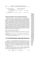
Figure 3.3.1:The solution to Laplace’s equation subject to the boundary conditions given
by Equation 3.3.2, Equation 3.3.3, and Equation 3.3.4 when a =0.5.
Figure 3.3.1 illustrates this solution when a =0.5.
• Example 3.3.2
Asimilar problem
18
to the previous one arises during the solution of
Laplace’s equation in cylindrical coordinates:
∂

2
u
∂r
2
+
1
r
∂u
∂r
+
∂
2
u
∂z
2
=0, 0 ≤ r<1, 0 <z<∞, (3.3.12)
subject to the boundary conditions
lim
r→0
|u(r, z)| < ∞,u
r
(1,z)=0, 0 <z<∞, (3.3.13)

u(r, 0) = 1, 0 ≤ r<a,
u
z
(r, 0) = 0,a<r<1,
(3.3.14)
and
lim

z→∞
|u
z
(r, z)| < ∞, 0 ≤ r<1, (3.3.15)
where a<1.
Separation of variablesgives
u(r, z)=A
0
z +
∞

n=1
A
n
e
−k
n
z
J
0
(k
n
r)
k
n
, (3.3.16)
18
SeeHunter, A., and A. Williams, 1969: Heat flow across metallic joints – The con-
striction alleviation factor. Int. J. Heat Mass Transfer, 12, 524–526.
© 2008 by Taylor & Francis Group, LLC

112 Mixed Boundary Value Problems
where k
n
is the nth positive root of J

0
(k)=−J
1
(k)=0. Equation 3.3.16
satisfies Equation 3.3.12, Equation 3.3.13, and Equation 3.3.15. Substituting
Equation 3.3.16 into Equation 3.3.14, we obtain the dual series:
∞

n=1
A
n
J
0
(k
n
r)
k
n
=1, 0 ≤ r<a, (3.3.17)
and
A
0
−
∞


n=1
A
n
J
0
(k
n
r)=0,a<r<1. (3.3.18)
Srivastav
19
has given the solution to the dual Fourier-Bessel series
αa
0
+
∞

n=1
a
n
J
0
(k
n
r)
k
n
= f(r), 0 ≤ r<a, (3.3.19)
and
a
0

+
∞

n=1
a
n
J
0
(k
n
r)=0,a<r<1. (3.3.20)
Then,
a
0
=2

a
0
h(t) dt, (3.3.21)
and
a
n
=
2
J
2
0
(k
n
)


a
0
h(t)cos(k
n
t) dt, (3.3.22)
where the function h(t)isgivenbythe integral equation
h(t) −

a
0
K(t, τ)h(τ) dτ = x(t), 0 <t<a, (3.3.23)
x(t)=
2
π
d
dt


t
0
rf(r)
√
t
2
− r
2
dr

, (3.3.24)

and
K(t, τ)=
4
π
(1 − α)+
4
π
2

∞
0
K
1
(ξ)
ξI
1
(ξ)
[2I
1
(ξ) −ξ cosh(τξ)cosh(tξ)] dξ.
(3.3.25)
19
Ibid. See also Sneddon, op. cit., Equation 5.3.27 through Equation 5.3.35.
© 2008 by Taylor & Francis Group, LLC
Separation of Variables 113
0
0.2
0.4
0.6
0.8

1
0
0.2
0.4
0.6
0.8
1
−1
−0.5
0
0.5
1
1.5
2
r
z
u(r,z)
Figure 3.3.2:The solution to Laplace’s equation subject to the boundary conditions given
by Equation 3.3.13 through Equation 3.3.15 when a =
1
2
.
Equation 3.3.19 through Equation 3.3.25 provide the answer to our problem
if we set α =0andf(r)=1. Figure 3.3.2 illustrates the solution when a =
1
2
.
• Example 3.3.3
Let us solve Laplace equation
20

∂
2
u
∂r
2
+
1
r
∂u
∂r
+
∂
2
u
∂z
2
=0, 0 ≤ r<a, 0 <z<∞, (3.3.26)
subject to the boundary conditions
lim
r→0
|u(r, z)| < ∞,u(a, z)=0, 0 <z<∞, (3.3.27)

u
z
(r, 0) = 1, 0 ≤ r<1,
u
r
(r, 0) = 0, 1 <r<a,
(3.3.28)
and

lim
z→∞
u(r, z) → 0, 0 ≤ r<a, (3.3.29)
where a>1.
The method of separation of variables yields the product solution
u(r, z)=
∞

n=1
A
n
J
0
(k
n
r)e
−k
n
z
, (3.3.30)
20
See Sherwood, J. D., and H. A. Stone, 1997: Added mass of a disc accelerating within
apipe.Phys. Fluids, 9, 3141–3148.
© 2008 by Taylor & Francis Group, LLC
114 Mixed Boundary Value Problems
where k
n
is the nth root of J
1
(ka)=0. Equation 3.3.30 satisfies not only

Laplace’s equation, but also the boundary conditions given by Equation 3.3.27
andEquation 3.3.29. Substituting Equation 3.3.30 into Equation 3.3.28, we
obtain the dual series
∞

n=1
A
n
k
n
J
0
(k
n
r)=−1, 0 ≤ r<1, (3.3.31)
and
∞

n=1
A
n
k
n
J
1
(k
n
r)=0, 1 ≤ r<a. (3.3.32)
We b egin our solution of these dual equations by applying the identity
21

∞

n=1
J
ν+2m+1−p
(ζ
n
)J
ν
(ζ
n
r)
ζ
1−p
n
J
2
ν+1
(ζ
n
a)
=0, 1 <r<a, (3.3.33)
where |p|≤
1
2
, ν>p− 1, m =0, 1, 2, ,andζ
n
denotes the nth root of
J
ν

(ζa)=0. Bydirection substitution it is easily seen that Equation 3.3.32 is
satisfied if ν =1and
k
2−p
n
J
2
2
(k
n
a)A
n
=
∞

m=0
C
m
J
2m+2−p
(k
n
). (3.3.34)
Here p is still a free parameter. Substituting Equation 3.3.34 into Equation
3.3.31,
∞

n=1
∞


m=0
C
m
J
2m+2−p
(k
n
)J
0
(k
n
r)
k
1−p
n
J
2
2
(k
n
a)
= −1, 0 ≤ r<1. (3.3.35)
Our remaining task is to compute C
m
.Although Equation 3.3.35 holds
for any r between 0 and 1, it would be better if we did not have to deal with
its presence. It can be eliminated as follows: From Sneddon’s book,
22

∞

0
η
1−k
J
ν+2m+k
(η)J
ν
(rη) dη =
Γ(ν + m +1)r
ν
(1 − r
2
)
k−1
2
k−1
Γ(ν +1)Γ(m + k)
P
(k+ν,ν+1)
m

r
2

(3.3.36)
21
Tranter, C. J., 1959: On the analogies between some series containing Bessel functions
and certain special cases of the Weber-Schafheitlin integral. Quart. J. Math., Ser. 2, 10,
110–114.
22

Sneddon, op. cit., Equation 2.1.33 and Equation 2.1.34.
© 2008 by Taylor & Francis Group, LLC
Separation of Variables 115
if 0 ≤ r<1; this integral equals 0 if 1 <r<∞.HereP
(a,b)
m
(x)=
2
F
1
(−m, a+
m; b; x)istheJacobi polynomial. If we view Equation 3.3.36 as a Hankel
transform of η
−k
J
ν+2m+k
(η), then its inverse is
η
−k
J
ν+2m+k
(η)
=

1
0
Γ(ν + m +1)r
1+ν

1 − r

2

k−1
2
k−1
Γ(ν +1)Γ(m + k)
J
ν
(rη)P
(k+ν,ν+1)
m

r
2

dr. (3.3.37)
We also have from the orthogonality condition
23
of Jacobi polynomials that

1
0
r
2ν+1

1 − r
2

k−1
P

(k+ν,ν+1)
m

r
2

dr =
Γ(ν +1)Γ(k)
2Γ(ν + k +1)
δ
0m
, (3.3.38)
where δ
nm
is the Kronecker delta. Multiplying both sides of Equation 3.3.35
by r

1 − r
2

−p
P
(1−p,1)
m
(r
2
)andapplying Equation 3.3.38, we obtain
−
Γ(1 − p)
2Γ(2 −p)

δ
0j
=
∞

n=1
∞

m=0
C
m
J
2m+2−p
(k
n
)J
2j+1−p
(k
n
)Γ(j +1− p)
2
p
Γ(j +1)k
2−2p
n
J
2
2
(k
n

a)
;
(3.3.39)
or
∞

m=0
A
jm
C
m
= B
j
,j=0, 1, 2, , (3.3.40)
where
A
jm
=
∞

n=1
J
2m+2−p
(k
n
)J
2j+1−p
(k
n
)

k
2−2p
n
J
2
2
(k
n
a)
, (3.3.41)
and
B
j
=

−2
p−1
/Γ(2 − p),j=0,
0, otherwise.
(3.3.42)
For a given p,wecan solve Equation 3.3.40 after we truncate the infinite num-
ber of equations to just M .Foragivenk
n
we solve the truncated Equation
3.3.40, which yields C
m
for m =0, 1, 2, ,M.ThenEquation3.3.34 gives
A
n
.Finally, the potential u(r, z)follows from Equation 3.3.30. Figure 3.3.3

illustrates this solution when a =2andp =0.5.
• Example 3.3.4
In the previous example we solved Laplace’s equation over a semi-infinite
right cylinder. Here, let us solve Laplace’s equation
24
when the cylinder has
23
See page 83 in Magnus, W., and F. Oberhettinger, 1954: Formulas and Theorems for
the Functions of Mathematical Physics. Chelsea Publ. Co., 172 pp.
24
SeeGalceran,J., J. Cecilia, E. Companys, J. Salvador, and J. Puy, 2000: Analytical
expressions for feedback currents at the scanning electrochemical microscope. J. Phys.
Chem., Ser. B, 104, 7993-8000.
© 2008 by Taylor & Francis Group, LLC
Separation of Variables 117
and
∞

n=1
A
n
J
0
(k
n
r)=0, 1 ≤ r<a. (3.3.49)
Let us reexpress A
n
as follows:
A

n
=
1
√
k
n
J
2
1
(k
n
a)
∞

m=0
B
m
J
2m+
1
2
(k
m
). (3.3.50)
Substituting Equation 3.3.50 into Equation 3.3.49, we have
25
that
∞

n=1

A
n
J
0
(k
n
r)=
∞

m=o
B
m

∞

n=1
J
2m+
1
2
(k
m
)J
0
(k
n
r)
√
k
n

J
2
1
(k
n
a)

=0 (3.3.51)
for 1 <r≤ a.Therefore, Equation 3.3.49 is satisfied identically with this
definition of A
n
.
Next, we substitute Equation 3.3.50 into Equation 3.3.48, multiply both
sides of the resulting equation by rF
21

−s, s +
1
2
, 1,r
2

dr/
√
1 − r
2
and in-
tegrate between r =0andr =1.Wefind that
∞


m=0
C
m,s
B
m
=
√
2Γ(s +1)
Γ

s +
1
2


1
0
r
√
1 − r
2
F
21

−s, s +
1
2
, 1,r
2


dr (3.3.52)
=


2/π, s =0,
0,s>0,
(3.3.53)
where
C
m,s
=
∞

n=1
coth(k
n
b)J
2m+
1
2
(k
n
)J
2s+
1
2
(k
n
)
k

2
n
J
2
1
(k
n
a)
(3.3.54)
and s =0, 1, 2, Weused
J
2s+
1
2
(k
n
)
√
k
n
=
√
2Γ(s +1)
Γ

s +
1
2



1
0
r
√
1 − r
2
F
21

−s, s +
1
2
, 1,r
2

J
0
(k
n
r) dr.
(3.3.55)
Equation 3.3.55 is now solved to yield B
m
.Next,wecompute A
n
from Equa-
tion 3.3.50. Finally u(r, z)follows from Equation 3.3.47.
Figure 3.3.4 illustrates the solution to Equation 3.3.43 through Equa-
tion 3.3.46 when a =2andb =1. Assuggested by Galceran et al.,
26

the
25
Tranter, op. cit.
26
Galceran, Cecilia, Companys, Salvador, and Puy, op. cit.
© 2008 by Taylor & Francis Group, LLC
Separation of Variables 119
z
r
z = h
z = 0
1
a
Figure 3.3.5:Schematicof a hollow cylinder containing discs at z =0andz = h.
u(r, 0
−
)=u(r, 0
+
),u(r, h
−
)=u(r, h
+
), 0 ≤ r<a, (3.3.60)

u(r, 0) = G(r),u(r, h)=F (r), 0 ≤ r<1,
u
z
(r, 0
−
)=u

z
(r, 0
+
),u
z
(r, h
−
)=u
z
(r, h
+
), 1 <r<a,
(3.3.61)
and
lim
|z|→∞
u(r, z) → 0, 0 ≤ r<a. (3.3.62)
Here, G(r)andF (r)denotetheprescribed potential on the discs at z =0
and z = h,respectively. The parameters h
+
and h
−
denote points that are
slightly above or below h,respectively.
Separation of variables yields the potential, namely
u(r, z)=
∞

n=0
A

n
e
−k
n
(z−h)
J
0
(k
n
r)
k
n
,h≤ z<∞, (3.3.63)
u(r, z)=
∞

n=0

A
n
sinh(k
n
z)
sinh(k
n
h)
+ B
n
sinh[k
n

(h −z)]
sinh(k
n
h)

J
0
(k
n
r)
k
n
, 0 ≤ z ≤ h,
(3.3.64)
and
u(r, z)=
∞

n=0
B
n
e
k
n
z
J
0
(k
n
r)

k
n
, −∞ <z≤ 0, (3.3.65)
© 2008 by Taylor & Francis Group, LLC
120 Mixed Boundary Value Problems
where k
n
is the nth positive root of J
0
(ka)=0. Equation 3.3.63 through
Equation 3.3.65 satisfy Equation 3.3.58, Equation 3.3.59, Equation 3.3.60,
andEquation 3.3.62. Substituting Equation 3.3.63 through Equation 3.3.65
into Equation 3.3.61, we obtain the following system of simultaneous dual
series equations:
∞

n=0
A
n
J
0
(k
n
r)
k
n
= F (r), 0 ≤ r<1, (3.3.66)
∞

n=0

B
n
J
0
(k
n
r)
k
n
= G(r), 0 ≤ r<1, (3.3.67)
∞

n=0

[1 + coth(k
n
h)]A
n
−
B
n
sinh(k
n
h)

J
0
(k
n
r)=0, 1 <r<a, (3.3.68)

and
∞

n=0

[1 + coth(k
n
h)]B
n
−
A
n
sinh(k
n
h)

J
0
(k
n
r)=0, 1 <r<a. (3.3.69)
For 0 ≤ r<1, let us augment Equation 3.3.68 and Equation 3.3.69 with
∞

n=0

[1 + coth(k
n
h)]A
n

−
B
n
sinh(k
n
h)

J
0
(k
n
r)=−
1
r
d
dr


1
r
tg(t)
√
t
2
− r
2
dt

,
(3.3.70)

and
∞

n=0

[1 + coth(k
n
h)]B
n
−
A
n
sinh(k
n
h)

J
0
(k
n
r)=−
1
r
d
dr


1
r
th(t)

√
t
2
− r
2
dt

,
(3.3.71)
where g(t)andh(t)areunknown functions.
Taken together, Equation 3.3.68 through Equation 3.3.71 are a Fourier-
Bessel series over the interval 0 ≤ r<a.FromEquation 1.4.16 and Equation
1.4.17, it follows that
[1 + coth(k
n
h)]A
n
−
B
n
sinh(k
n
h)
= −
2
a
2
J
2
1

(k
n
a)

1
0
d
dr


1
r
tg(t)
√
t
2
− r
2
dt

J
0
(k
n
r) dr (3.3.72)
= −
2
a
2
J

2
1
(k
n
a)


1
r
tg(t)
√
t
2
− r
2
dt

J
0
(k
n
r)




1
0
−
2

a
2
J
2
1
(k
n
a)

1
0
k
n
J
1
(k
n
r)


1
r
tg(t)
√
t
2
− r
2
dt


dr (3.3.73)
=
2
a
2
J
2
1
(k
n
a)

1
0
g(t) dt
−
2k
n
a
2
J
2
1
(k
n
a)

1
0
tg(t)



t
0
J
1
(k
n
r)
√
t
2
− r
2
dr

dt. (3.3.74)
© 2008 by Taylor & Francis Group, LLC
Separation of Variables 121
Now,

t
0
J
1
(k
n
r)
√
t

2
− r
2
dr =

1
0
J
1
(k
n
tη)

1 − η
2
dη =
π
2
J
2
1
2
(k
n
t/2) =
1 − cos(k
n
t)
k
n

t
, (3.3.75)
where weusedtables
29
to evaluate the integral. Therefore,
[1 + coth(k
n
h)]A
n
−
B
n
sinh(k
n
h)
=
2
a
2
J
2
1
(k
n
a)

1
0
g(t)cos(k
n

t) dt. (3.3.76)
In a similar manner,
[1 + coth(k
n
h)]B
n
−
A
n
sinh(k
n
h)
=
2
a
2
J
2
1
(k
n
a)

1
0
h(t)cos(k
n
t) dt. (3.3.77)
Solving for A
n

and B
n
,wefind that
A
n
=
1
a
2
J
2
1
(k
n
a)


1
0
g(t)cos(k
n
t) dt + e
−k
n
h

1
0
h(t)cos(k
n

t) dt

,
(3.3.78)
and
B
n
=
1
a
2
J
2
1
(k
n
a)


1
0
h(t)cos(k
n
t) dt + e
−k
n
h

1
0

g(t)cos(k
n
t) dt

.
(3.3.79)
Substituting A
n
and B
n
into Equation 3.3.66 and 3.3.67 and interchanging
the order of integration and summation,

1
0
g(t)

∞

n=0
J
0
(k
n
r)cos(k
n
t)
a
2
k

n
J
2
1
(k
n
a)

dt
+

1
0
h(t)

∞

n=0
e
−k
n
h
J
0
(k
n
r)cos(k
n
t)
a

2
k
n
J
2
1
(k
n
a)

dt = F (r), (3.3.80)
and

1
0
h(t)

∞

n=0
J
0
(k
n
r)cos(k
n
t)
a
2
k

n
J
2
1
(k
n
a)

dt
+

1
0
g(t)

∞

n=0
e
−k
n
h
J
0
(k
n
r)cos(k
n
t)
a

2
k
n
J
2
1
(k
n
a)

dt = G(r). (3.3.81)
29
Gradshteyn and Ryzhik, op. cit., Formula 6.552.4.
© 2008 by Taylor & Francis Group, LLC
122 Mixed Boundary Value Problems
It is readily shown
30
that
2
a
2
∞

n=0
J
0
(k
n
r)cos(k
n

t)
k
n
J
2
1
(k
n
a)
=

∞
0
J
0
(rη)cos(tη) dη
−
2
π

∞
0
K
0
(aη)
I
0
(aη)
I
0

(rη)cosh(tη)dη. (3.3.82)
In a similar manner,
2
a
2
∞

n=0
e
−k
n
h
J
0
(k
n
r)cos(k
n
t)
k
n
J
2
1
(k
n
a)
=

∞

0
J
0
(rη)cos(tη)e
−hη
dη (3.3.83)
−
2
π

∞
0
K
0
(aη)
I
0
(aη)
I
0
(rη)cosh(tη)cos(hη)dη.
Substituting Equation 1.4.14, Equation 3.3.82, and Equation 3.3.83 into Equa-
tion 3.3.80 and Equation 3.3.81, we have that

r
0
g(t)
√
r
2

− t
2
dt =
2
π

1
0
g(t)


∞
0
K
0
(aη)
I
0
(aη)
I
0
(rη)cosh(tη)dη

dt
−
2
π

1
0

h(t)


∞
0
K
0
(aη)
I
0
(aη)
I
0
(rη)cosh(tη)cos(hη)dη

dt
−

1
0
h(t)


∞
0
J
0
(rη)cos(tη)e
−hη
dη


dt +2F (r), (3.3.84)
and

r
0
h(t)
√
r
2
− t
2
dt =
2
π

1
0
h(t)


∞
0
K
0
(aη)
I
0
(aη)
I

0
(rη)cosh(tη) dη

dt
−
2
π

1
0
g(t)


∞
0
K
0
(aη)
I
0
(aη)
I
0
(rη)cosh(tη)cos(hη) dη

dt
−

1
0

g(t)


∞
0
J
0
(rη)cos(tη)e
−hη
dη

dt +2G(r). (3.3.85)
Equation 3.3.84 and Equation 3.3.85 are integral equations of the Abel type.
From Equation 1.2.13 and Equation 1.2.14, we find
g(t)=
4
π
d
dt


t
0
rF(r)
√
t
2
− r
2
dr


+
4
π
2

1
0
g(ξ)


∞
0
K
0
(aη)
I
0
(aη)
cosh(tη)cosh(ξη) dη

dξ
+
4
π
2

1
0
h(ξ)



∞
0
K
0
(aη)
I
0
(aη)
cosh(tη)cosh(ξη)cos(hη)dη

dξ
−
2
π

1
0
h(ξ)


∞
0
e
−hη
cos(ξη)cos(tη) dη

dξ, (3.3.86)
30

See Section 2.2inSneddon, op. cit.
© 2008 by Taylor & Francis Group, LLC
Separation of Variables 123
0
0.5
1
1.5
2
−2
−1
0
1
2
3
4
−1
−0.5
0
0.5
1
r
z
u(r,z)
Figure 3.3.6:The electrostatic potential within an infinitely long, grounded, and hollow
cylinder of radius 2 when two discs with potential −1and1areplaced at z =0andz =2,
respectively.
and
h(t)=
4
π

d
dt


t
0
rG(r)
√
t
2
− r
2
dr

+
4
π
2

1
0
g(ξ)


∞
0
K
0
(aη)
I

0
(aη)
cosh(tη)cosh(ξη)cos(hη)dη

dξ
+
4
π
2

1
0
h(ξ)


∞
0
K
0
(aη)
I
0
(aη)
cosh(tη)cosh(ξη) dη

dξ
−
2
π


1
0
g(ξ)


∞
0
e
−hη
cos(ξη)cos(tη) dη

dξ. (3.3.87)
ForagivenF(r)andG(r), we solve the integral equations Equation 3.3.86
and Equation3.3.87 for g(t)andh(t). Equation 3.3.78 and Equation 3.3.79
give A
n
and B
n
.Finally, we can use Equation 3.3.63through Equation 3.3.65
to evaluate the potential for any given r and z.Figure 3.3.6 illustrates the
electrostatic potential when F(r)=1,G(r)=−1, and a = h =2.
• Example 3.3.6: Electrostatic problem
In electrostatics the potential due to a point charge located at r =0and
z = h in the upper half-plane z>0above agrounded plane z =0is
u(r, z)=
1

r
2
+(z −h)

2
−
1

r
2
+(z + h)
2
. (3.3.88)
Let us introduce a unit circular hole at z =0andattach an infinite pipe to
© 2008 by Taylor & Francis Group, LLC
124 Mixed Boundary Value Problems
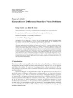
(0,h)
z
r
(1,0)
Figure 3.3.7:Schematic of the spatial domain for which we are finding the potential in
Example 3.3.6.
this hole. See Figure 3.3.7. Let us find the potential
31
in this case.
The potential in this new configuration is
u(r, z)=
1

r
2
+(z −h)
2
−

1

r
2
+(z + h)
2
+
1
2i

1
−1
g(t)

r
2
+(z + it)
2
dt
(3.3.89)
when 0 ≤ r<∞ and 0 ≤ z<∞ and
u(r, z)=
∞

n=1
A
n
J
0
(k

n
r)e
k
n
z
(3.3.90)
when 0 ≤ r ≤ 1and−∞ <z≤ 0. The integral
32
in Equation 3.3.89 vanishes
when z =0and1≤ r<∞.Hereg(t)isanoddreal-valued function and
k
n
denotes the nth root of J
0
(k)=0. Todetermineg(t)andtheFourier
coefficients A
n
,thepotentialand its normal derivativemustbecontinuous
across the aperture z =0and0≤ r ≤ 1. Mathematically these conditions
are
u(r, 0
−
)=u(r, 0
+
), 0 ≤ r ≤ 1, (3.3.91)
and
u
z
(r, 0
−

)=u
z
(r, 0
+
), 0 ≤ r ≤ 1. (3.3.92)
31
Takenfrom Shail, R., and B. A. Packham, 1986: Some potential problems associated
with the sedimentation of a small particle into a semi-infinite fluid-filled pore. IMA J. Appl.
Math., 37, 37–66 with permission of Oxford University Press.
32
See Section 5.10 in Green, A. E., and W. Zerna, 1992: Theoretical Elasticity. New
York: Dover, 457 pp.
© 2008 by Taylor & Francis Group, LLC
Separation of Variables 125
Equation 3.3.91 yields
∞

n=1
A
n
J
0
(k
n
r)=−

1
r
g(t)
√

t
2
− r
2
dt, 0 ≤ r ≤ 1. (3.3.93)
In deriving Equation 3.3.93, we used

r
2
+(z + it)
2
= ξe
iη/2
,

r
2
+(z −it)
2
= ξe
−iη/2
, (3.3.94)
with ξ
2
cos(η)=r
2
+ z
2
− t
2

, ξ
2
sin(η)=2zt, ξ ≥ 0, and 0 ≤ η ≤ π.Onthe
other hand, Equation 3.3.92 gives
1
r
∂
∂r


r
0
th(t)
√
r
2
− t
2
dt

=
∞

n=1
k
n
A
n
J
0

(k
n
r) −
2h
(r
2
+ h
2
)
3/2
, 0 ≤ r ≤ 1.
(3.3.95)
Using Equation 1.2.13 and Equation 1.2.14, we can solve for g(t)inEquation
3.3.93 and find that
g(t)=
2
π
∞

n=1
k
n
A
n

t
0
rJ
0
(k

n
r)
√
t
2
− r
2
dr −
4h
π

t
0
r

(t
2
− r
2
)(r
2
+ h
2
)
3
dr
(3.3.96)
=
2
π

∞

n=1
A
n
sin(k
n
t) −
4t
π(t
2
+ h
2
)
, 0 ≤ t ≤ 1. (3.3.97)
We used Equation 1.4.9 and tables
33
to evaluate the integrals in Equation
3.3.96.
Substituting the results from Equation 3.3.97 into Equation 3.3.95, we
obtain
∞

n=1
A
n
J
0
(k
n

r)=−
2
π
∞

n=1
A
n

1
r
sin(k
n
t)
√
t
2
− r
2
dt +
4
π

1
r
t
(t
2
+ h
2

)
√
t
2
− r
2
dt.
(3.3.98)
The left side of Equation 3.3.98 is a Fourier-Bessel expansion. Multiplying
both sides ofthisequationbyrJ
0
(k
m
r)andintegrating with respect to r from
0to1,wefind that
1
2
J
2
1
(k
m
)A
m
= −
2
π
∞

n=1

A
n

1
0
rJ
0
(k
m
r)


1
r
sin(k
n
t)
√
t
2
− r
2
dt

dr
+
4
π

1

0
rJ
0
(k
m
r)


1
r
dt
(t
2
+ h
2
)
√
t
2
− r
2

dr. (3.3.99)
33
Gradshteyn and Ryzhik, op. cit., Formula 2.252, Point II.
© 2008 by Taylor & Francis Group, LLC
126 Mixed Boundary Value Problems
0
0.5
1

1.5
2
−2
−1
0
1
2
0
1
2
3
4
5
6
7
8
9
10
z
r
u(r,z)
Figure 3.3.8:Theelectrostatic potential when a unit point charge is placed at r =0and
z = h for the structure illustrated in Figure 3.3.7.
Interchanging the order of integration in Equation 3.3.99 and evaluating the
inner r integrals, we finally achieve
1
2
πJ
2
1

(k
m
)A
m
+
∞

n=1
A
n

sin(k
n
− k
m
)
k
n
− k
m
−
sin(k
n
+ k
m
)
k
n
+ k
m


=4

1
0
t
t
2
+ h
2
sin(k
m
t) dt, (3.3.100)
where m =1, 2, 3, Tofind A
m
,wetruncate the infinite number of equa-
tions given by Equation 3.3.100 to a finite number, say M.AsM increases
the A
m
’s with a smaller m increase in accuracy. The procedure is stopped
when the leading A
m
’s are sufficiently accurate fortheevaluation of Equation
3.3.89, Equation 3.3.90 and Equation 3.3.97. Figure 3.3.8 illustrates this so-
lution when h =1andthefirst 300 terms have been retained when M = 600.
3.4 DUAL FOURIER-LEGENDRE SERIES
Here we turn to problems in spherical coordinates which lead to dual
Fourier-Legendre series. We now present severalexamplesoftheir solution.
© 2008 by Taylor & Francis Group, LLC
Separation of Variables 127

• Example 3.4.1
Let us solve
34
the axisymmetric Laplace equation within the unit sphere:
∂
∂r

r
2
∂u
∂r

+
1
sin(θ)
∂
∂θ

sin(θ)
∂u
∂θ

=0, 0 ≤ r<1, 0 <θ<π, (3.4.1)
subject to the boundary conditions
lim
θ→0
|u(r, θ)| < ∞, lim
θ→π
|u(r, θ)| < ∞, 0 ≤ r ≤ 1, (3.4.2)
lim

r→0
|u(r, θ)| < ∞, 0 ≤ θ ≤ π, (3.4.3)
and

u(1,θ)=1, 0 ≤ θ<α,
u
r
(1,θ)=−bu(1,θ),α<θ≤ π.
(3.4.4)
Separation of variables yields the solution
u(r, θ)=
∞

n=0
A
n
r
n
P
n
[cos(θ)]. (3.4.5)
Equation 3.4.5 satisfies not only Equation 3.4.1, but also Equation 3.4.2 and
Equation 3.4.3. Substituting Equation 3.4.5 into Equation 3.4.4 yields the
dual Fourier-Legendre series
∞

n=0
A
n
P

n
[cos(θ)] = 1, 0 ≤ θ<α, (3.4.6)
and
∞

n=0
(b + n)A
n
P
n
[cos(θ)] = 0,α≤ θ<π. (3.4.7)
Consider Equation 3.4.6. Using Equation 1.3.4 to eliminate P
n
[cos(θ)]
and then interchanging the order of integration and summation, we have

θ
0
1

cos(ϕ) −cos(θ)

∞

n=0
A
n
cos

n +

1
2

ϕ


dϕ =
π
√
2
, 0 ≤ ϕ<α.
(3.4.8)
Applying the results from Equation 1.2.9 and Equation 1.2.10,
∞

n=0
A
n
cos

n +
1
2

ϕ

=
1
√
2

d
dϕ


ϕ
0
sin(τ)

cos(τ) − cos(ϕ)
dτ

(3.4.9)
=
√
2
d
dϕ


1 − cos(ϕ)

(3.4.10)
=cos(ϕ/2). (3.4.11)
34
See Ramachandran, M. P., 1993: A note on the integral equation method to a diffusion-
reaction problem. Appl. Math. Lett., 6, 27–30.
© 2008 by Taylor & Francis Group, LLC
128 Mixed Boundary Value Problems
In a similar manner, Equation 3.4.7 can be rewritten as


π
θ
1

cos(θ) − cos(ϕ)

∞

n=0
(b + n)A
n
sin

n +
1
2

ϕ


dϕ =0 (3.4.12)
for α<θ≤ π.Therefore,
∞

n=0
(b + n)A
n
sin

n +

1
2

ϕ

=
∞

n=0

n +
1
2
− γ

A
n
sin

n +
1
2

ϕ

=0
(3.4.13)
with α<ϕ≤ π and γ =
1
2

− b.IntegratingEquation 3.4.13 with respect to
ϕ,wehave
∞

n=0

1 −
γ
n +
1
2

A
n
cos

n +
1
2

ϕ

=0. (3.4.14)
The constant of integration equals zero because the left side of Equation 3.4.14
vanishes when ϕ = π.
At this point, let us supplement Equation 3.4.11 with
ψ(ϕ)=
∞

n=0

A
n
cos

n +
1
2

ϕ

,α<ϕ≤ π. (3.4.15)
Therefore, Equation 3.4.14 can be rewritten
ψ(ϕ) − γ
∞

n=0
A
n
cos

n +
1
2

ϕ

n +
1
2
=0. (3.4.16)

From the definition of half-range Fourier series,
A
n
=
2
π

α
0
cos( ˜ϕ/2) cos

n +
1
2

˜ϕ

d ˜ϕ +
2
π

π
α
ψ(˜ϕ)cos

n +
1
2

˜ϕ


d ˜ϕ
(3.4.17)
=
sin(nα)
nπ
+
sin[(n +1)α]
(n +1)π
+
2
π

π
α
ψ(˜ϕ)cos

n +
1
2

˜ϕ

d ˜ϕ. (3.4.18)
Substituting Equation 3.4.18 into Equation 3.4.16 and interchanging the order
of integration and summation,
ψ(ϕ)=
2γ
π



α
0
cos( ˜ϕ/2)

∞

n=0
cos

n +
1
2

ϕ

cos

n +
1
2

˜ϕ

n +
1
2

d ˜ϕ
+


π
α
ψ(˜ϕ)

∞

n=0
cos

n +
1
2

ϕ

cos

n +
1
2

˜ϕ

n +
1
2

d ˜ϕ


. (3.4.19)
© 2008 by Taylor & Francis Group, LLC
Separation of Variables 129
Because
35
∞

n=0
cos

n +
1
2

ϕ

cos

n +
1
2

˜ϕ

n +
1
2
=
1
2

ln

cos( ˜ϕ/2) + cos(ϕ/2)
cos( ˜ϕ/2) −cos(ϕ/2)

, (3.4.20)
Equation 3.4.19 becomes
ψ(ϕ)=
γ
π

α
0
cos( ˜ϕ/2)L(˜ϕ, ϕ) d ˜ϕ +
γ
π

π
α
ψ(˜ϕ)L(˜ϕ, ϕ) d ˜ϕ, (3.4.21)
where
L(˜ϕ, ϕ)=ln




cos( ˜ϕ/2) + cos(ϕ/2)
cos( ˜ϕ/2) −cos(ϕ/2)





. (3.4.22)
To simplify Equation 3.4.21, we set ψ(ϕ)=cos(ϕ/2) + r(ϕ)anditbecomes
r(ϕ) −
γ
π

π
α
r(˜ϕ)L(˜ϕ, ϕ) d ˜ϕ =(2γ −1) cos(ϕ/2),α<ϕ≤ π. (3.4.23)
To numerically solve Equation 3.4.23, we introduce n nodal points at
ϕ
i
= α + ih, i =0, 1, ,n− 1, where h =(π − α)/n.Wedonothaveto
compute r(π)becauseitequals zero since ψ(π)=0fromEquation 3.4.15.
Then, Equation 3.4.23 becomes
r(ϕ
i
) −
γ
π

π
α
r(t)L(t, ϕ
i
) dt =(2γ − 1) cos(ϕ
i
/2), (3.4.24)

where
L(t, ϕ)=ln


2cos[(t + ϕ)/4]


+ln


cos(t −ϕ)/4


(3.4.25)
− ln


2sin[(t + ϕ)/4]


− ln




sin[(t − ϕ)/4]
t − ϕ





− ln


t − ϕ


.
Why have we written L(t, ϕ)intheformgiveninEquation 3.4.25? It
clearly shows that the integral equation, Equation 3.4.23, contains a weakly
singular kernel. Consequently, the finite difference representation of the inte-
gral in Equation 3.4.24 consists of two parts. A simple trapezoidal rule is used
for the first four terms given in Equation 3.4.25. For the fifth term, we em-
ploy a numerical method devised by Atkinson
36
for kernels with singularities.
Therefore, for a particular alpha and b,wecompute dt = (pi-alpha)/N,
35
Parihar, K. S., 1971: Some triple trigonometrical series equations and their applica-
tion. Proc. R. Soc. Edinburgh, Ser. A, 69, 255–265.
36
Atkinson, K. E., 1967: The numerical solution of Fredholm integral equations of the
second kind. SIAM J. Numer. Anal., 4, 337–348. See Section 5 in particular.
© 2008 by Taylor & Francis Group, LLC
130 Mixed Boundary Value Problems
where N is the number of nodal points. The M
ATLAB code for computing
ψ(ϕ)is
for j = 0:N
tt(j+1) = alpha + j*dt;

pphi(j+1) = alpha + j*dt;
end
% Solve the integral equation Equation 3.4.24 to find r(ϕ
i
).
% Note that r(π)=0.
for n = 0:N-1 % rows loop (top to bottom in the matrix)
phi = pphi(n+1); bb(n+1) = (2*gamma-1)*cos(phi/2);
for m = 0:N-1 % columns loop (left to right in the matrix)
t=tt(m+1);
% Introduce the first terms from Equation 3.4.24.
if (n==m) AA(n+1,m+1) = 1;
else AA(n+1,m+1) = 0; end
% Compute integral in Equation 3.4.24. Add in the contribution
% from the first four terms of Equation 3.4.25. Use the
% trapezoidal rule. Recall that r(π)=0.
if (m < N)
arg
1=(t+phi)/4; arg 2=(t-phi)/4;
AA(n+1,m+1) = AA(n+1,m+1)
- 0.5*dt*gamma*log(abs(2*cos(arg
1)))/pi
- 0.5*dt*gamma*log(abs(cos(arg
2)))/pi
+ 0.5*dt*gamma*log(abs(2*sin(arg
1)))/pi;
if (arg
2==0)
AA(n+1,m+1) = AA(n+1,m+1) + 0.5*dt*gamma*log(0.25)/pi;
else

AA(n+1,m+1) = AA(n+1,m+1)
+ 0.5*dt*gamma*log(abs(sin(arg
2)/(t-phi)))/pi;
end
end
if (m > 0)
arg
1=(t+phi)/4; arg 2=(t-phi)/4;
AA(n+1,m+1) = AA(n+1,m+1)
© 2008 by Taylor & Francis Group, LLC
Separation of Variables 131
- 0.5*dt*gamma*log(abs(2*cos(arg
1)))/pi
- 0.5*dt*gamma*log(abs(cos(arg
2)))/pi
+ 0.5*dt*gamma*log(abs(2*sin(arg
1)))/pi;
if (arg
2==0)
AA(n+1,m+1) = AA(n+1,m+1) + 0.5*dt*gamma*log(0.25)/pi;
else
AA(n+1,m+1) = AA(n+1,m+1)
+ 0.5*dt*gamma*log(abs(sin(arg
2)/(t-phi)))/pi;
end
end
% Use Atkinson’s technique to treat the fifth term in
% Equation 3.4.25. See Section 5 of his paper.
if (m > 0)
kk = n+1-m; Psi

0=-1;
Psi
1=0.25*(kk*kk-(kk-1)*(kk-1));
if(kk∼=0)
Psi
0=Psi 0+kk*log(abs(kk));
Psi
1=Psi 1-0.50*kk*kk*log(abs(kk));
end
if(kk∼=1)
Psi
0=Psi 0-(kk-1)*log(abs(kk-1));
Psi
1=Psi 1+0.50*(kk-1)*(kk-1)*log(abs(kk-1));
end
Psi
1=Psi 1+kk*Psi 0;
W
0=Psi 0-Psi 1; W 1=Psi 1;
aalpha = 0.5*dt*log(dt) + dt*W
0;
bbeta = 0.5*dt*log(dt) + dt*W
1;
AA(n+1,m ) = AA(n+1,m ) + gamma*aalpha/pi;
AA(n+1,m+1) = AA(n+1,m+1) + gamma*bbeta/pi;
end
end % end of column loop
end % end of rows loop
% compute r(ϕ
i

)
r=AA\bb

% compute ψ(ϕ)
for n = 0:N-1
theta = tt(n+1); psi(n+1) = cos(theta/2) + r(n+1);
end
© 2008 by Taylor & Francis Group, LLC
132 Mixed Boundary Value Problems
Once ψ(ϕ
i
)isfound with ψ(π)=0,wecompute A
n
via Equation 3.4.18. The
M
ATLAB code to compute A
n
is
for m = 0:M
if(m==0)
A(m+1) = alpha/pi + sin(alpha)/pi;
else
A(m+1) = sin(m*alpha)/(m*pi) + sin((m+1)*alpha)/((m+1)*pi);
end
% This is the n =0 term for Simpson’s rule.
A(m+1) = A(m+1) + 2*psi( 1 )*cos((m+0.5)*tt( 1 ))*dt/(3*pi);
% Recall that ψ(π)=0. Therefore, we do not need then=N
% term in the numerical integration.
for n = 1:N-1
if ( mod(n+1,2) == 0 )

A(m+1) = A(m+1) + 8*psi(n+1)*cos((m+0.5)*tt(n+1))*dt/(3*pi);
else
A(m+1) = A(m+1) + 4*psi(n+1)*cos((m+0.5)*tt(n+1))*dt/(3*pi);
end; end; end
The final solution follows from Equation 3.4.5. The M
ATLAB code to realize
this solution is
for j = 1:41
y=0.05*(j-21);
for i = 1:41
x=0.05*(i-21);
u(i,j) = NaN; r = sqrt(x*x + y*y); theta = abs(atan2(y,x));
if (r <= 1)
mu = cos(theta);
% Compute the Legendre polynomials for a given theta
% via the recurrence formula
Legendre(1) = 1; Legendre(2) = mu;
for m = 2:M
Legendre(m+1) = (2-1/m)*mu*Legendre(m) - (1-1/m)*Legendre(m-1);
end
% For a point within the sphere, find the solution.
u(i,j) = 0; power = 1;
for m = 0:M
u(i,j) = u(i,j) + A(m+1)*Legendre(m+1)*power;
© 2008 by Taylor & Francis Group, LLC
Separation of Variables 133
−1
−0.5
0
0.5

1
−1
−0.5
0
0.5
1
−0.2
0
0.2
0.4
0.6
0.8
1
x
y
u(r,θ )
Figure 3.4.1:Thesolutionu(r, θ)tothe mixed boundary value problem posed in Example
3.4.1 with α = π/4andb =0.25.
power = power*r;
end; end; end; end
Figure 3.4.1 illustrates the solution when α = π/4andb =0.25.
An alternative method for solving Equation 3.4.6 and Equation 3.4.7 is
to introduce the following integral definition for A
n
:
A
n
=
2n +1
n + b


α
0
h(t)cos

n +
1
2

t

dt. (3.4.26)
Integration by parts gives
(n+b)A
n
=2h(α)sin

n +
1
2

α

−2

α
0
h

(t)sin


n +
1
2

t

dt. (3.4.27)
Then,
∞

n=0
(n + b)A
n
P
n
[cos(θ)] = 2h(α)
∞

n=0
sin

n +
1
2

α

P
n

[cos(θ)] (3.4.28)
− 2

α
0
h

(t)

∞

n=0
sin

n +
1
2

t

P
n
[cos(θ)]

dt
=0. (3.4.29)
Therefore, our choice for the A
n
satisfies Equation 3.4.7 identically. Here we
used results from Problem 1 at the end of Section 1.3.

© 2008 by Taylor & Francis Group, LLC
134 Mixed Boundary Value Problems
Turning to Equation 3.4.6, we have for A
n
that
∞

n=0
n +
1
2
n + b
P
n
[cos(θ)]

α
0
h(t)cos

n +
1
2

t

dt =
1
2
. (3.4.30)

Breaking the summation on the left side of Equation 3.4.30 into two parts,
we can rewrite it as
∞

n=0
P
n
[cos(θ)]

α
0
h(t)cos

n +
1
2

t

dt (3.4.31)
=
1
2
−
∞

n=0
γ
n + b
P

n
[cos(θ)]

α
0
h(τ)cos

n +
1
2

τ

dτ.
On the left side of Equation 3.4.31, we interchange the order of integration and
summation and employ again the results from Problem 1. Equation 3.4.31
simplifies to

θ
0
h(t)

2[cos(t) − cos(θ)]
dt (3.4.32)
=
1
2
−
∞


n=0
γ
n + b
P
n
[cos(θ)]

α
0
h(τ)cos

n +
1
2

τ

dτ.
Upon employing Equation 1.2.9 and Equation 1.2.10, we can solve for h(t)
and find that
h(t)=
1
π
d
dt


t
0
sin(θ)


2[cos(θ) − cos(t)]
dθ

−
2
π

α
0
h(τ)

∞

n=0
γ
n + b
cos

n +
1
2

τ

(3.4.33)
×
d
dt



t
0
sin(θ)P
n
[cos(θ)]

2[cos(θ) − cos(t)]
dθ


dτ
=
1
π
d
dt


2[1 −cos(t)]

(3.4.34)
−
2
π

α
0
h(τ)


∞

n=0
γ
n + b
cos

n +
1
2

τ

cos

n +
1
2

t


dt.
We used resultsfromProblem 2 at the end of Section 1.3 to evaluate the
integral within the wavy brackets in Equation 3.4.33. Therefore, we now have
the Fredholm integral equation
h(t)+

α
0

[K(t − τ)+K(t + τ)]h(τ) dτ =
sin(t)
π

2[1 −cos(t)]
, (3.4.35)
© 2008 by Taylor & Francis Group, LLC