Tài liệu Two Point Boundary Value Problems part 1 pptx
Bạn đang xem bản rút gọn của tài liệu. Xem và tải ngay bản đầy đủ của tài liệu tại đây (78.5 KB, 5 trang )
Sample page from NUMERICAL RECIPES IN C: THE ART OF SCIENTIFIC COMPUTING (ISBN 0-521-43108-5)
Copyright (C) 1988-1992 by Cambridge University Press.Programs Copyright (C) 1988-1992 by Numerical Recipes Software.
Permission is granted for internet users to make one paper copy for their own personal use. Further reproduction, or any copying of machine-
readable files (including this one) to any servercomputer, is strictly prohibited. To order Numerical Recipes books,diskettes, or CDROMs
visit website or call 1-800-872-7423 (North America only),or send email to (outside North America).
Chapter 17. Two Point Boundary
Value Problems
17.0 Introduction
When ordinarydifferentialequations arerequired tosatisfy boundaryconditions
at more than one value of the independent variable, the resulting problem is called a
two point boundary value problem. As the terminology indicates, the most common
case by far is where boundaryconditions are supposed to be satisfied at two points —
usually the starting and ending values of the integration. However, the phrase “two
point boundary value problem” is also used loosely to include more complicated
cases, e.g., where some conditions are specified at endpoints, others at interior
(usually singular) points.
The crucial distinction between initial value problems (Chapter 16) and two
point boundary value problems (this chapter) is that in the former case we are able
to start an acceptable solution at its beginning (initialvalues) and just march it along
by numerical integration to its end (final values); while in the present case, the
boundary conditions at the starting point do not determine a unique solution to start
with — and a “random” choice among the solutions that satisfy these (incomplete)
starting boundary conditions is almost certain not to satisfy the boundary conditions
at the other specified point(s).
It should not surprise you that iteration is in general required to meld these
spatially scattered boundaryconditionsintoa singleglobal solutionof the differential
equations. For this reason, two point boundary value problems require considerably
more effort to solve than do initial value problems. You have to integrate your dif-
ferential equations over the interval of interest, or perform an analogous “relaxation”
procedure (see below), at least several, and sometimes very many, times. Only in
the special case of linear differential equations can you say in advance just how
many such iterations will be required.
The “standard” two point boundary value problem has the following form: We
desire the solution to a set of N coupled first-order ordinary differential equations,
satisfying n
1
boundary conditions at the starting point x
1
, and a remaining set of
n
2
= N − n
1
boundary conditions at the final point x
2
. (Recall that all differential
equations of order higher than first can be written as coupled sets of first-order
equations, cf. §16.0.)
The differential equations are
dy
i
(x)
dx
= g
i
(x, y
1
,y
2
,...,y
N
) i=1,2,...,N (17.0.1)
753
754
Chapter 17. Two Point Boundary Value Problems
Sample page from NUMERICAL RECIPES IN C: THE ART OF SCIENTIFIC COMPUTING (ISBN 0-521-43108-5)
Copyright (C) 1988-1992 by Cambridge University Press.Programs Copyright (C) 1988-1992 by Numerical Recipes Software.
Permission is granted for internet users to make one paper copy for their own personal use. Further reproduction, or any copying of machine-
readable files (including this one) to any servercomputer, is strictly prohibited. To order Numerical Recipes books,diskettes, or CDROMs
visit website or call 1-800-872-7423 (North America only),or send email to (outside North America).
required
boundary
value
desired
boundary
value
1
3
2
y
x
Figure 17.0.1. Shooting method(schematic). Trial integrations that satisfy theboundary condition at one
endpointare “launched.” The discrepanciesfrom the desired boundarycondition at the other endpointare
used to adjust the starting conditions,until boundaryconditionsat bothendpointsare ultimately satisfied.
At x
1
, the solution is supposed to satisfy
B
1j
(x
1
,y
1
,y
2
,...,y
N
)=0 j=1,...,n
1
(17.0.2)
while at x
2
, it is supposed to satisfy
B
2k
(x
2
,y
1
,y
2
,...,y
N
)=0 k=1,...,n
2
(17.0.3)
There are two distinct classes of numerical methods for solving two point
boundary value problems. In the shooting method (§17.1) we choose values for all
of the dependent variables at one boundary. These values must be consistent with
any boundary conditions for that boundary, but otherwise are arranged to depend
on arbitrary free parameters whose values we initially “randomly” guess. We then
integratetheODEsbyinitialvaluemethods,arrivingattheotherboundary(and/orany
interiorpoints with boundary conditionsspecified). In general, we find discrepancies
from the desired boundary values there. Now we have a multidimensional root-
finding problem, as was treated in §9.6 and §9.7: Find the adjustment of the free
parameters at the starting point that zeros the discrepancies at the other boundary
point(s). If we liken integrating the differential equations to following the trajectory
of a shot from gun to target, then pickingthe initialconditionscorresponds to aiming
(see Figure 17.0.1). The shooting method provides a systematic approach to taking
a set of “ranging” shots that allow us to improve our “aim” systematically.
As another variant of the shooting method (§17.2), we can guess unknown free
parameters at bothends of the domain, integrate the equations to a common midpoint,
and seek to adjust the guessed parameters so that the solution joins “smoothly” at
the fitting point. In all shooting methods, trial solutions satisfy the differential
equations “exactly” (or as exactly as we care to make our numerical integration),
but the trial solutions come to satisfy the required boundary conditions only after
the iterations are finished.
Relaxation methods use a different approach. The differential equations are
replaced by finite-difference equations on a mesh of points that covers the range of
17.0 Introduction
755
Sample page from NUMERICAL RECIPES IN C: THE ART OF SCIENTIFIC COMPUTING (ISBN 0-521-43108-5)
Copyright (C) 1988-1992 by Cambridge University Press.Programs Copyright (C) 1988-1992 by Numerical Recipes Software.
Permission is granted for internet users to make one paper copy for their own personal use. Further reproduction, or any copying of machine-
readable files (including this one) to any servercomputer, is strictly prohibited. To order Numerical Recipes books,diskettes, or CDROMs
visit website or call 1-800-872-7423 (North America only),or send email to (outside North America).
required
boundary
value
required
boundary
value
i
n
i
t
i
a
l
g
u
e
s
s
1
s
t
i
t
e
r
a
t
i
o
n
2
n
d
i
t
e
r
a
t
i
o
n
true solution
Figure 17.0.2. Relaxation method (schematic). An initial solution is guessed that approximately satisfies
the differential equation and boundary conditions. An iterative process adjusts the function to bring it
into close agreement with the true solution.
the integration. A trial solution consists of values for the dependent variables at each
mesh point,notsatisfyingthedesired finite-differenceequations,nornecessarily even
satisfying the required boundary conditions. The iteration, now called relaxation,
consists of adjusting all the values on the mesh so as to bring them into successively
closer agreement with the finite-difference equations and, simultaneously, with the
boundary conditions (see Figure 17.0.2). For example, if the problem involves three
coupled equations and a mesh of one hundred points, we must guess and improve
three hundred variables representing the solution.
With all this adjustment, you may be surprised that relaxation is ever an efficient
method, but (for the right problems) it really is! Relaxation works better than
shooting when the boundary conditions are especially delicate or subtle, or where
they involve complicated algebraic relations that cannot easily be solved in closed
form. Relaxation works best when the solution is smooth and not highly oscillatory.
Such oscillations would require many grid points for accurate representation. The
number and positionof required pointsmay not beknown apriori. Shootingmethods
are usually preferred in such cases, because their variable stepsize integrations adjust
naturally to a solution’s peculiarities.
Relaxation methods are often preferred when the ODEs have extraneous
solutions which, while not appearing in the final solution satisfying all boundary
conditions, may wreak havoc on the initial value integrations required by shooting.
The typical case is that of trying to maintain a dying exponential in the presence
of growing exponentials.
Good initial guesses are the secret of efficient relaxation methods. Often one
has to solve a problem many times, each time with a slightly different value of some
parameter. In that case, the previous solution is usually a good initial guess when
the parameter is changed, and relaxation will work well.
Until you have enough experience to make your own judgment between the two
methods, you might wish to follow the advice of your authors, who are notorious
computer gunslingers: We always shoot first, and only then relax.
756
Chapter 17. Two Point Boundary Value Problems
Sample page from NUMERICAL RECIPES IN C: THE ART OF SCIENTIFIC COMPUTING (ISBN 0-521-43108-5)
Copyright (C) 1988-1992 by Cambridge University Press.Programs Copyright (C) 1988-1992 by Numerical Recipes Software.
Permission is granted for internet users to make one paper copy for their own personal use. Further reproduction, or any copying of machine-
readable files (including this one) to any servercomputer, is strictly prohibited. To order Numerical Recipes books,diskettes, or CDROMs
visit website or call 1-800-872-7423 (North America only),or send email to (outside North America).
Problems Reducible to the Standard Boundary Problem
There are two important problems that can be reduced to the standard boundary
value problem described by equations (17.0.1) – (17.0.3). The first is the eigenvalue
problem for differential equations. Here the right-hand side of the system of
differential equations depends on a parameter λ,
dy
i
(x)
dx
= g
i
(x, y
1
,...,y
N
,λ)(17.0.4)
and one has to satisfy N +1boundary conditions instead of just N. The problem
is overdetermined and in general there is no solution for arbitrary values of λ.For
certain special values of λ, the eigenvalues, equation (17.0.4) does have a solution.
We reduce this problem to the standard case by introducing a new dependent
variable
y
N+1
≡ λ (17.0.5)
and another differential equation
dy
N+1
dx
=0 (17.0.6)
An example of this trick is given in §17.4.
The other case that can be put in the standard form is a free boundary problem.
Here only one boundary abscissa x
1
is specified, while the other boundary x
2
is to
be determined so that the system (17.0.1) has a solution satisfying a total of N +1
boundary conditions. Here we again add an extra constant dependent variable:
y
N+1
≡ x
2
− x
1
(17.0.7)
dy
N+1
dx
=0 (17.0.8)
We also define a new independent variable t by setting
x − x
1
≡ ty
N+1
, 0 ≤ t ≤ 1(17.0.9)
The system of N +1differential equations for dy
i
/dt is now in the standard form,
with t varying between the known limits 0 and 1.
CITED REFERENCES AND FURTHER READING:
Keller, H.B. 1968,
Numerical Methods for Two-Point Boundary-Value Problems
(Waltham, MA:
Blaisdell).
Kippenhan, R., Weigert, A., and Hofmeister, E. 1968, in
Methods in Computational Physics
,
vol. 7 (New York: Academic Press), pp. 129ff.
Eggleton, P.P. 1971,
Monthly Notices of the Royal Astronomical Society
, vol. 151, pp. 351–364.
London, R.A., and Flannery, B.P. 1982,
Astrophysical Journal
, vol. 258, pp. 260–269.
Stoer, J., and Bulirsch, R. 1980,
Introduction to Numerical Analysis
(New York: Springer-Verlag),
§§
7.3–7.4.
17.1 The Shooting Method
757
Sample page from NUMERICAL RECIPES IN C: THE ART OF SCIENTIFIC COMPUTING (ISBN 0-521-43108-5)
Copyright (C) 1988-1992 by Cambridge University Press.Programs Copyright (C) 1988-1992 by Numerical Recipes Software.
Permission is granted for internet users to make one paper copy for their own personal use. Further reproduction, or any copying of machine-
readable files (including this one) to any servercomputer, is strictly prohibited. To order Numerical Recipes books,diskettes, or CDROMs
visit website or call 1-800-872-7423 (North America only),or send email to (outside North America).
17.1 The Shooting Method
In this section we discuss “pure” shooting, where the integration proceeds from
x
1
to x
2
, and we try to match boundary conditions at the end of the integration. In
the next section, we describe shooting to an intermediate fitting point, where the
solution to the equations and boundary conditions is found by launching “shots”
from both sides of the interval and trying to match continuity conditions at some
intermediate point.
Our implementation of the shooting method exactly implements multidimen-
sional, globally convergent Newton-Raphson (§9.7). It seeks to zero n
2
functions
of n
2
variables. The functions are obtained by integrating N differential equations
from x
1
to x
2
. Let us see how this works:
At the starting point x
1
there are N starting values y
i
to be specified, but
subject to n
1
conditions. Therefore there are n
2
= N − n
1
freely specifiable starting
values. Let us imagine that these freely specifiable values are the components of a
vector V that lives in a vector space of dimension n
2
. Then you, the user, knowing
the functional form of the boundary conditions (17.0.2), can write a function that
generates a complete set of N starting values y, satisfying the boundary conditions
at x
1
, from an arbitrary vector value of V in which there are no restrictions on the n
2
component values. In other words, (17.0.2) converts to a prescription
y
i
(x
1
)=y
i
(x
1
;V
1
,...,V
n
2
) i=1,...,N (17.1.1)
Below, the function that implements (17.1.1) will be called load.
Notice that the components of V might be exactly the values of certain “free”
components of y, with the other components of y determined by the boundary
conditions. Alternatively, the components of V might parametrize the solutions that
satisfy the starting boundary conditions in some other convenient way. Boundary
conditions often impose algebraic relations among the y
i
, rather than specific values
for each of them. Using some auxiliary set of parameters often makes it easier to
“solve” the boundary relations for a consistent set of y
i
’s. It makes no difference
which way you go, as long as your vector space of V’s generates (through 17.1.1)
all allowed starting vectors y.
Given a particular V, a particular y(x
1
) is thus generated. It can then be turned
into a y(x
2
) by integrating the ODEs to x
2
as an initial value problem (e.g., using
Chapter 16’s odeint). Now, at x
2
, let us define a discrepancy vector F,alsoof
dimension n
2
, whose components measure how far we are from satisfying the n
2
boundary conditions at x
2
(17.0.3). Simplest of all is just to use the right-hand
sides of (17.0.3),
F
k
= B
2k
(x
2
, y) k =1,...,n
2
(17.1.2)
As in the case of V, however, you can use any other convenient parametrization,
as long as your space of F’s spans the space of possible discrepancies from the
desired boundary conditions, with all components of F equal to zero if and only if
the boundary conditions at x
2
are satisfied. Below, you will be asked to supply a
user-written function score which uses (17.0.3) to convert an N-vector of ending
values y(x
2
) into an n
2
-vector of discrepancies F.