Mixed Boundary Value Problems Episode 9 pptx

228 Mixed Boundary Value Problems
Substituting for A(k)from Equation 4.3.118 into Equation 4.3.119, we find
after interchanging the order of integration that
∂
∂t


∞
a
g(ξ)Q(ξ, t) dξ

=

∞
t
rf(r)
√
r
2
− t
2
dr, (4.3.120)
where
Q(ξ,t)=

∞
0
[J
1
(k)cos(kt)+Y
1

(k)sin(kt)]
J
2
1
(k)+Y
2
1
(k)
× [Y
1
(k)cos(kξ) − J
1
(kξ)sin(kξ)]
dk
k
, (4.3.121)
or
Q(ξ,t)=−
1
2


∞
0
sin[k(ξ −t)]
dk
k
−

∞

0
sin[k(ξ + t)]
dk
k
+ 


∞
0

H
(2)
1
(k)
H
(1)
1
(k)
+1

e
i(ξ+t)k
dk
k


. (4.3.122)
Our final task is to evaluate the contour integral

Γ


H
(2)
1
(z)
H
(1)
1
(z)
+1

e
i(ξ+t)z
dz
z
,
where the contour Γ consists of the real axis from the origin to R,anarcin
the first quadrant |z| = R,0≤ θ ≤ π/2, and imaginary axis from iR to the
origin. As R →∞,wefind that



∞
0

H
(2)
1
(k)
H

(1)
1
(k)
+1

e
i(ξ+t)k
dk
k

= −π

∞
0
I
1
(k)
K
1
(k)
e
−k(t+ξ)
dk
k
.
(4.3.123)
Therefore, Equation 4.3.120 becomes
1
2
∂

∂t

−
π
2

t
a
g(ξ) dξ +
π
2

∞
t
g(ξ) dξ (4.3.124)
−

∞
a
g(ξ)

π

∞
0
I
1
(k)
K
1

(k)
e
−k(t+ξ)
dk
k

dξ

=

∞
t
rf(r)
√
r
2
− t
2
dr,
or
g(t)+

∞
a
g(ξ)


∞
0
I

1
(k)
K
1
(k)
e
−k(t+ξ)
dk

dξ =
2
π

∞
t
rf(r)
√
r
2
− t
2
dr, (4.3.125)
© 2008 by Taylor & Francis Group, LLC
Transform Methods 229
0
5
10
15
20
0

5
10
15
20
−0.4
−0.3
−0.2
−0.1
0
0.1
r
z
u
z
(r,z)
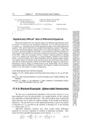
Figure 4.3.4:Thesolutionu(r, z)tothe mixed boundary value problem governed by
Equation 4.3.108 through Equation 4.3.111 with a =2.
for a<t<∞.Figure 4.3.4 illustrates the solution when a =2.
• Example 4.3.6
Let us solve
44
∂
2
u
∂r
2
+
1
r
∂u

∂r
+
1
z
p
∂
∂z

z
n
∂u
∂z

=0, 0 ≤ r<∞, 0 <z<∞, (4.3.126)
subject to the boundary conditions
lim
r→0
|u(r, z)| < ∞, lim
r→∞
u(r, z) → 0, 0 <z<∞, (4.3.127)
lim
z→∞
u(r, z) → 0, 0 ≤ r<∞, (4.3.128)
and

u(r, 0) = 1, 0 ≤ r<1,
z
n
u
z

(r, z)


z=0
=0, 1 <r<∞,
(4.3.129)
where κ>0.
44
TakenfromBrutsaert, W., 1967: Evaporation from a very small water surface at
ground level: Three-dimensional turbulent diffusion without convection. J. Geophys. Res.,
72, 5631–5639.
c
1967 American Geophysical Union. Reproduced/modified by permission
of American Geophysical Union.
© 2008 by Taylor & Francis Group, LLC
230 Mixed Boundary Value Problems
Using transform methods or separation of variables, the general solution
to Equation 4.3.126, Equation 4.3.127, and Equation 4.3.128 is
u(r, z)=z
(1−n)/2

∞
0
A(k)K
ν

2νk
1 − n
z
(1−n)/(2ν)


J
0
(kr) dk, (4.3.130)
where ν =(1− n)/(p − n +2). Substituting Equation 4.3.130 into Equation
4.3.129, we have that

∞
0
A(k)J
0
(kr)
dk
k
ν
= C, 0 ≤ r<1, (4.3.131)
and

∞
0
k
ν
A(k)J
0
(kr) dk =0, 1 <r<∞, (4.3.132)
where
C =
2
Γ(ν)


ν
1 − n

ν
. (4.3.133)
If we now restrict ν so that it lies between 0 and
1
4
,then
A(k)=
(2k)
ν
C
Γ(1 − ν)

k
1−ν
J
−ν
(k)

1
0
η
(1 − η
2
)
ν
dη
+



1
0
ζ
(1 − ζ
2
)
ν
dζ


1
0
(kη)
2−ν
J
1−ν
(kη) dη

(4.3.134)
=
2
ν−1
kC
Γ(2 − ν)
[J
−ν
(k)+J
2−ν

(k)] (4.3.135)
=2
ν+1

ν
1 − n

ν
sin(νπ)
π
J
1−ν
(k). (4.3.136)
Consequently, the final solution is
u(r, z)=

2
ν+1

ν
1 − n

ν
sin(νπ)
π

z
(1−n)/2
×


∞
0
K
ν

2νk
1 − n
z
(1−n)/(2ν)

J
0
(kr)J
1−ν
(k) dk. (4.3.137)
Figure 4.3.5 illustrates this solution when n =
1
2
and p =1.
• Example 4.3.7
Let us solve
45
∂
2
u
∂r
2
+
1
r

∂u
∂r
−
u
r
2
+
∂
2
u
∂z
2
= κ
2
u, 0 ≤ r<∞, 0 <z<∞, (4.3.138)
45
Asimplified version of a problem solved by Borodachev, N. M., and Yu. A.Mamteyew,
1969: Unsteady torsional oscillations of an elastic half-space. Mech. Solids, 4(1), 79–83.
© 2008 by Taylor & Francis Group, LLC
232 Mixed Boundary Value Problems
Setting x = r/a, ξ = ka,andg(ξ)=

ξ
2
+(κa)
2
A(ξ)inEquation4.3.143
and Equation 4.3.144, we find that

∞

0
g(ξ)

ξ
2
+(κa)
2
J
1
(ξx) dξ = x, 0 ≤ x<1, (4.3.145)
and

∞
0
g(ξ)J
1
(ξx) dξ =0, 1 <x<∞. (4.3.146)
By comparing our problem with the canonical form given by Equation 4.3.26
through Equation 4.3.27, then ν =1andG(ξ)=

ξ
2
+(κa)
2

−1/2
.Selecting
a =1,α = −
1
2

,andβ =
1
2
,then
g(ξ)=
4ξ
π

1
0
h(t)sin(ξt) dt, (4.3.147)
and
h(t)+

1
0
K(t, η)h(η) dη = t, 0 ≤ t ≤ 1, (4.3.148)
where
K(t, η)=
2
π

1
0

1 −
ξ

ξ
2

+(κa)
2

sin(tξ)sin(ηξ) dξ (4.3.149)
=
2
π

1
0


ξ
2
− (κa)
2
− ξ

ξ
2
+(κa)
2

sin(tξ)sin(ηξ) dξ (4.3.150)
=
2
π
(κa)
2


1
0
sin(tξ)sin(ηξ)

ξ
2
+(κa)
2

ξ +

ξ
2
+(κa)
2

dξ (4.3.151)
=
κa
2
{L
1
[κa(η + t)] − I
1
[κa(η + t)]
− L
1
[κa|η − t|]+I
1
[κa|η − t|]}, (4.3.152)

where L
1
(·)denotes a modified Struve function of the first kind. Vasudevaiah
and Majhi
46
showed how to evaluate the integral in Equation 4.3.151.
As in the previousexamples,wemust solve for h(x)numerically. Then
g(ξ)iscomputed from Equation 4.3.147. Finally, Equation 4.3.142 gives
u(r, z). Figure 4.3.6 illustrates this solution when κa =1.
46
Vasudevaiah, M., and S. N. Majhi, 1981: Viscous impulsive rotation of two finite
coaxial disks. Indian J. Pure Appl. Math., 12, 1027–1042.
© 2008 by Taylor & Francis Group, LLC
234 Mixed Boundary Value Problems
Substituting Equation 4.3.157 into Equation 4.3.156, we have that

∞
0

k
2
− α
2
A(k)J
0
(kr) dk =1, 0 ≤ r<a, (4.3.158)
and

∞
0

A(k)J
0
(kr) dk =0,a<r<∞. (4.3.159)
To solve the dual integral equations, Equation 4.3.158 and Equation
4.3.159, we set
kA(k)=
2
π

a
0
h(t)[cos(kt) − cos(ka)] dt. (4.3.160)
We chose this definition for A(k)because

∞
0
A(k)J
0
(kr) dk =
2
π

a
0
h(t)


∞
0
[cos(kt) − cos(ka)]J

0
(kr)
dk
k

dt =0,
(4.3.161)
where wehaveintegratedEquation1.4.13 with respect to t from 0 and a after
setting ν =0andnoted that 0 ≤ t ≤ a<r.
Turning to Equation 4.3.158, we substitute Equation 4.3.160 into Equa-
tion 4.3.158. This yields

a
0
h(t)

2
π

∞
0

k
2
− α
2
[cos(kt) − cos(ka)]J
0
(kr)
dk

k

dt =1, 0 ≤ r<a,
(4.3.162)
or

a
0
h(t)

2
π

∞
0
[cos(kt) − cos(ka)]J
0
(kr) dk

dt (4.3.163)
−

a
0
h(t)

2
π

∞

0

1 −
√
k
2
− α
2
k

[cos(kt) − cos(ka)]J
0
(kr) dk

dt =1.
Let us evaluate
2
π

∞
0

1 −
√
k
2
− α
2
k


[cos(kt) − cos(ka)]J
0
(kr) dk
=
4
π
2

π/2
0

∞
0

1 −
√
k
2
− α
2
k

[cos(kτ) − cos(ka)] cos[kr sin(θ)] dk dθ
(4.3.164)
=
2
π
2

π/2

0

∞
0

1 −
√
k
2
− α
2
k


cos{k[τ − r sin(θ)]}−cos{k[a − r sin(θ)]}
+cos{k[t + r sin(θ)]}−cos{k[a + r sin(θ)]}

dk dθ. (4.3.165)
© 2008 by Taylor & Francis Group, LLC
Transform Methods 235
We used the integraldefinition of J
0
(kr)toobtain Equation 4.3.164.
Consider now the integral
L =
2
π

∞
0


1 −
√
k
2
− κ
2
k

[cos(kα) − cos(kβ)] dk, α, β > 0. (4.3.166)
Then
∂L
∂α
= −
2
π

∞
0

k −

k
2
− κ
2

sin(kα) dk (4.3.167)
=
2

πα

∞
0

k −

k
2
− κ
2

d[cos(kα)] (4.3.168)
=
2
πα

iκ −

∞
0

1 −
k
√
k
2
− κ
2


cos(kα) dk

(4.3.169)
=
2
πα

iκ −
d
dα


∞
0
sin(kα)
k
dk

+
d
dα


∞
0
sin(kα)
√
k
2
− κ

2
dk

(4.3.170)
=
2
πα

iκ +
d
dα


∞
0
sin(kα)
√
k
2
− κ
2
dk

. (4.3.171)
Using the integral representation for the Bessel and Struve functions
48
J
0
(x)=
2

π

∞
1
sin(xt)
√
t
2
− 1
dt, H
0
(x)=
2
π

1
0
sin(xt)
√
1 − t
2
dt, (4.3.172)
with J

0
(x)=−J
1
(x)andH

0

(x)=2/π − H
1
(x), we obtain the final result
that
∂L
∂α
= −
κ
α
[J
1
(κα) − iH
1
(κα)] . (4.3.173)
Upon integrating Equation 4.3.173 with respect to α and noting that L =0
when α = β,wefind that
2
π

∞
0

1 −
√
k
2
− κ
2
k


[cos(kα) − cos(kβ)] dk = κ

Ji
1
(κβ) − Ji
1
(κα)
− i [Hi
1
(κβ) − Hi
1
(κα)]

,
(4.3.174)
if α, β > 0, where
Ji
1
(x)=

x
0
J
1
(y)
dy
y
, and Hi
1
(x)=


x
0
H
1
(y)
dy
y
. (4.3.175)
48
Gradshteyn and Ryzhik, op. cit., Formula 8.411.9 and Formula 8.551.1.
© 2008 by Taylor & Francis Group, LLC
236 Mixed Boundary Value Problems
0
0.5
1
1.5
2
−1
−0.5
0
0.5
1
−0.8
−0.6
−0.4
−0.2
0
0.2
0.4

0.6
r
z
u(r,z)
Figure 4.3.7:Thesolutionu(r, z)tothe mixed boundary value problem governed by
Equation 4.3.153 through Equation 4.3.156 with a =1andα =0.1.
Applying these results to Equation 4.3.163, we have
2
π

r
0
h(t)
√
r
2
− t
2
dt −
2α
π

π/2
0

a
0
K[r sin(θ),τ]h(τ) dτ dθ =1 (4.3.176)
with
K(r, τ)=

1
2

Ji
1
[α(a − r)] − Ji
1
[α|t − r|]+Ji
1
[α(a + r)] − Ji
1
[α(t + r)]
− iHi
1
[α(a − r)] + iHi
1
[α|t − r|] − iHi
1
[α(a + r)] + iHi
1
[α(t + r)]

.
(4.3.177)
Because

r
0
h(t)
√

r
2
− t
2
dt =

π/2
0
h[r sin(θ)] dθ, (4.3.178)
Equation 4.3.176 can be rewritten
2
π

π/2
0

h[r sin(θ)] − α

a
0
K[r sin(θ),τ]h(τ) dτ

dθ =1, 0 ≤ r<a.
(4.3.179)
Equation 4.3.179 is satisfied if
h(x) − α

a
0
K(x, τ)h(τ) dτ =1, 0 ≤ x ≤ a. (4.3.180)

Figure 4.3.7 illustrates u(r, z)whena =1andα =0.1.
© 2008 by Taylor & Francis Group, LLC
Transform Methods 237
In a similar manner,
49
we can solve
∂
2
u
∂r
2
+
1
r
∂u
∂r
+
∂
2
u
∂z
2
+

α
2
−
1
r
2


u =0, 0 ≤ r<∞, −∞ <z<∞,
(4.3.181)
subject to the boundary conditions
lim
r→0
|u(r, z)| < ∞, lim
r→∞
u(r, z) → 0, −∞ <z<∞, (4.3.182)
lim
|z|→∞
u(r, z) → 0, 0 ≤ r<∞, (4.3.183)
and

u(r, 0
−
)=u(r, 0
+
)=r, 0 ≤ r<a,
u
z
(r, 0
−
)=u
z
(r, 0
+
),a<r<∞.
(4.3.184)
Using transform methods or separation of variables, the general solution

to Equation 4.3.181, Equation 4.3.182, and Equation 4.3.183 is
u(r, z)=

∞
0
A(k)J
1
(kr)e
−|z|
√
k
2
−α
2
dk. (4.3.185)
Substituting Equation 4.3.185 into Equation 4.3.184, we have that

∞
0
A(k)J
1
(kr) dk = r, 0 ≤ r<a, (4.3.186)
and

∞
0

k
2
− α

2
A(k)J
1
(kr) dk =0,a<r<∞. (4.3.187)
We can satisfy Equation 4.3.187 identically if we set
A(k)=
2k
π
√
k
2
− α
2

a
0
h(t)sin(kt) dt, (4.3.188)
because

∞
0

k
2
− α
2
A(k)J
1
(kr) dk =


a
0
h(t)


∞
0
k sin(kt)J
1
(kr) dk

dt
(4.3.189)
= −

1
0
h(t)
d
dr


∞
0
sin(kt)J
0
(kr) dk

dt =0
(4.3.190)

49
See also Ufliand, Ia. S., 1961: On torsional vibrations of half-space. J. Appl. Math.
Mech., 25, 228–233.
© 2008 by Taylor & Francis Group, LLC
238 Mixed Boundary Value Problems
since the integral within the square brackets vanishes in Equation 4.3.190
when 0 ≤ t ≤ a<r.
Turning Equation 4.3.186, we substitute Equation 4.3.188 into it. This
yields

a
0
h(t)

2
π

∞
0
k
√
k
2
− α
2
sin(kt)J
1
(kr) dk

dt = r, 0 ≤ r<a, (4.3.191)

or

a
0
h(t)

2
π

∞
0
sin(kt)J
1
(kr) dk

dt (4.3.192)
−

a
0
h(t)

2
π

∞
0

1 −
k

√
k
2
− α
2

sin(kt)J
1
(kr) dk

dt = r.
Let us evaluate
2
π

∞
0

1 −
k
√
k
2
− α
2

sin(kt)J
1
(kr) dk
=

4
π
2

π/2
0
sin(θ)


∞
0

1 −
k
√
k
2
− α
2

sin(kt)sin[kr sin(θ)] dk

dθ
(4.3.193)
=
2
π
2

π/2

0
sin(θ)


∞
0

1 −
k
√
k
2
− α
2

cos{k[τ − r sin(θ)]}
− cos{k[t + r sin(θ)]}

dk

dθ. (4.3.194)
We used the integraldefinition of J
1
(kr)toobtain Equation 4.3.193.
Consider now the integral
L =
2
π

∞

0

1 −
k
√
k
2
− κ
2

cos(kα) dk, α > 0. (4.3.195)
Then,
L =
d
dα

2
π

∞
0

1 −
k
√
k
2
− κ
2


sin(kα)
dk
k

(4.3.196)
= −
d
dα

2
π

∞
0
sin(kα)
√
k
2
− κ
2
dk

(4.3.197)
= κ

J
1
(κα) − iH
1
(κα)+

2i
π

. (4.3.198)
Applying these results to Equation 4.3.194, we find
2
πr

r
0
th(t)
√
r
2
− t
2
dt −
2α
π

π/2
0


a
0
K[r sin(θ),τ]h(τ) dτ

sin(θ) dθ = r
(4.3.199)

© 2008 by Taylor & Francis Group, LLC
Transform Methods 239
0
0.5
1
1.5
2
−1
−0.5
0
0.5
1
0
0.1
0.2
0.3
0.4
0.5
0.6
0.7
0.8
0.9
1
r
z
u(r,z)
Figure 4.3.8:Thesolutionu(r, z)tothe mixed boundary value problem governed by
Equation 4.3.181 through Equation 4.3.184 with a =1andα =0.1.
with
K(r, τ)=

1
2
{J
1
[α|τ − r|] − J
1
[α(t + r)] − iH
1
[α|t − r|]+iH
1
[α(t + r)]}.
(4.3.200)
Because
2
πr

r
0
th(t)
√
r
2
− t
2
dt =
2
π

π/2
0

h[r sin(θ)] sin(θ) dθ, (4.3.201)
Equation 4.3.199 can be written
2
π

π/2
0

h[r sin(θ)] − α

a
0
K[r sin(θ),τ]h(τ) dτ

sin(θ) dθ = r (4.3.202)
with 0 ≤ r<a.Ifweset
h(x) − α

a
0
K(x, τ)h(τ) dτ = f(x), 0 ≤ x ≤ a, (4.3.203)
then Equation 4.3.202 becomes
2
π

π/2
0
r sin(θ)f[r sin(θ)] dθ = r
2
(4.3.204)

which has thesolutionf(x)=2x.Therefore, h(t)isgivenby
h(x) − α

a
0
K(x, τ)h(τ) dτ =2x, 0 ≤ x ≤ a. (4.3.205)
Figure 4.3.8 illustrates u(r, z)whena =1andα =0.1.
© 2008 by Taylor & Francis Group, LLC
240 Mixed Boundary Value Problems
• Example 4.3.9
Let us solve
50
∂
2
u
∂r
2
+
1
r
∂u
∂r
+
∂
2
u
∂z
2
− α
2

u =0, 0 ≤ r<∞, −h<z<∞, (4.3.206)
subject to the boundary conditions
lim
r→0
|u(r, z)| < ∞, lim
r→∞
u(r, z) → 0, −h<z<∞, (4.3.207)
lim
z→∞
u(r, z) → 0, 0 ≤ r<∞, (4.3.208)
u
r
(r, −h)=0, 0 ≤ r<∞, (4.3.209)
u
r
(r, 0
−
)=u
r
(r, 0
+
), 0 ≤ r<∞, (4.3.210)
and

u
r
(r, 0
−
)=u
r

(r, 0
+
)=−r, 0 ≤ r<1,
u
rz
(r, 0
−
)=u
rz
(r, 0
+
), 1 <r<∞.
(4.3.211)
Using transform methods or separation of variables, the general solution
to Equation 4.3.206 through Equation 4.3.210 is
u(r, z)=

∞
0
A(k)e
−λz
J
0
(kr)
dk
k
, 0 <z<∞, (4.3.212)
and
u(r, z)=


∞
0
A(k)
sinh[λ(z + h)]
sinh(λh)
J
0
(kr)
dk
k
, −h<z<0, (4.3.213)
where λ =
√
k
2
+ α
2
with (λ) > 0. Substituting Equation 4.3.212 and
Equation 4.3.213 into Equation 4.3.211, we have that

∞
0
B(k)

1 − e
−2λh

J
1
(kr)

dk
λ
= −2r, 0 ≤ r<1, (4.3.214)
and

∞
0
B(k)J
1
(kr) dk =0, 1 ≤ r<∞, (4.3.215)
where
B(k)=−
λe
λh
A(k)
sinh(λh)
. (4.3 .216)
50
See Chu, J. H., and M U. Kim, 2004: Oscillatory Stokes flow due to motions of a
circular disk parallel to an infinite plane wall. Fluid Dyn. Res., 34, 77–97.
© 2008 by Taylor & Francis Group, LLC
Transform Methods 241
To solve the dual integral equations, Equation 4.3.214 and Equation
4.3.215, we introduce
B(k)=k

1
0
h(t)sin(kt) dt. (4.3.217)
Following Equation 4.3.189 and Equation 4.3.190, we can show that this choice

satisfies Equation 4.3.215 identically.
Turning to Equation 4.3.214, we substitute Equation 4.3.217 into Equa-
tion 4.3.214. This yields

1
0
h(t)


∞
0
sin(kt)J
1
(kr) dk

dt (4.3.218)
−

1
0
h(t)

sin(kt)J
1
(kr) −
k
λ

1 − e
−2λh


sin(kt)J
1
(kr) dk

dt = −2r.
From integral tables,
51

∞
0
J
1
(αx)sin(βx) dx =

β
α
√
α
2
−β
2
,α>β,
0,α<β,
(4.3.219)
we can evaluate the first term in Equation 4.3.218 and this equation now reads

r
0
th(t)

r
√
r
2
− t
2
dt (4.3.220)
=

1
0
h(τ)


∞
0

1 −
k
λ
+
k
λ
e
−2λh

sin(kτ)J
1
(kr) dk


dτ − 2r.
Upon applying the results from Equation 1.2.13 and Equation 1.2.14,
rh(r)=
2
π

1
0
h(τ)


∞
0

1 −
k
λ
+
k
λ
e
−2λh

× sin(kτ)
d
dr


r
0

ξ
2
J
1
(kξ)

r
2
− ξ
2
dξ

dk

dτ
−
4
π
d
dr


r
0
ξ
3

r
2
− ξ

2
dξ

. (4.3.221)
Now
−
4
π
d
dr


r
0
ξ
3

r
2
− ξ
2
dξ

= −
8r
2
π
, (4.3.222)
51
Gradshteyn and Ryzhik, op. cit., Formula 6.671.

© 2008 by Taylor & Francis Group, LLC
242 Mixed Boundary Value Problems
0
0.5
1
1.5
2
−1
−0.5
0
0.5
1
0
0.1
0.2
0.3
0.4
0.5
0.6
0.7
0.8
z/h
r/h
u(r,z)
Figure 4.3.9:Thesolutionu(r, z)tothe mixed boundary value problem governed by
Equation 4.3.206 through Equation 4.3.211 with h =1andα =1.
and
d
dr



r
0
ξ
2
J
1
(kξ)

r
2
− ξ
2
dξ

= r sin(kr)(4.3.223)
after using integral tables.
52
Substituting these results into Equation 4.3.221
and dividing by r,
h(r) −
2
π

1
0
h(τ)


∞

0

1 −
k
λ
+
k
λ
e
−2λh

sin(kτ)sin(kr) dk

dτ = −
8r
π
.
(4.3.224)
Figure 4.3.9 illustrates u(r, z)whenh =1andα =1.
• Example 4.3.10
In the previous examples, the boundary condition was u(r, 0) = 0 or
u
z
(r, 0) = 0 for 0 <a<r<∞.Inthisexampleweconsider the other
situation where u(r, 0) = 0 applies when 0 <r<1. In particular, we find the
solution
53
to
∂
2

u
∂r
2
+
1
r
∂u
∂r
+
∂
2
u
∂z
2
=0, 0 ≤ r<∞, 0 <z<h, (4.3.225)
52
Ibid., Formula 6.567.1 with ν =1andµ = −
1
2
.
53
TakenfromDhaliwal, R. S., 1967: An axisymmetric mixed boundary value problem
for a thick slab. SIAM J. Appl. Math., 15, 98–106.
c
1967 Society for Industrial and
Applied Mathematics. Reprinted with permission.
© 2008 by Taylor & Francis Group, LLC
Transform Methods 243
subject to the boundary conditions
lim

r→0
|u(r, z)| < ∞, lim
r→∞
u(r, z) → 0, 0 <z<h, (4.3.226)
u
z
(r, h)=0, 0 ≤ r<∞, (4.3.227)
and

u(r, 0) = 0, 0 ≤ r<1,
u
z
(r, 0) = −f (r), 1 <r<∞.
(4.3.228)
Using transform methods or separation of variables, the general solution
to Equation 4.3.225, Equation 4.3.226, and Equation 4.3.227 is
u(r, z)=

∞
0
A(k)
cosh[k(z −h)]
cosh(kh)
J
0
(kr) dk. (4.3.229)
Substituting Equation 4.3.229 into Equation 4.3.228, we have that

∞
0

A(k)J
0
(kr) dk =0, 0 ≤ r<1, (4.3.230)
and

∞
0
kA(k)tanh(kh)J
0
(kr) dk = f(r), 1 <r<∞. (4.3.231)
To solve Equation 4.3.230 and Equation 4.3.231, we set
A(k)=

∞
1
g(t)cos(kt) dt, (4.3.232)
where lim
t→∞
g(t) → 0. We didthisbecause

∞
0
A(k)J
0
(kr) dk =

∞
1
g(t)



∞
0
cos(kt)J
0
(kr) dk

dt =0 (4.3.233)
from Equation 1.4.14 with 0 <r<1 ≤ t<∞.Turning to Equation 4.3.231,
the substitution of Equation 4.3.232 yields

∞
0
J
0
(kr)


∞
1
kg(t)cos(kt) dt

dk (4.3.234)
−

∞
0
kM(kh)J
0
(kr)



∞
1
g(t)cos(kt) dt

dk = f(r),
where M(kh)=2/

1+e
2kh

.
© 2008 by Taylor & Francis Group, LLC
244 Mixed Boundary Value Problems
We now simplify Equation 4.3.234 in two ways. In the first term we
integrate by parts the integral within the square brackets and apply Equation
1.4.13. We then replace J
0
(kr)byitsintegral representation.
54
This gives
−

∞
r
g

(t)
√

t
2
− r
2
dt −
2
π

∞
0
kM(kh)


∞
r
sin(kt)
√
t
2
− r
2
dt

(4.3.235)
×


∞
1
g(x)cos(kx) dx


dk = f (r).
Interchanging the order of integration and using the trigonometric product
formula, Equation 4.3.235 becomes

∞
r

g

(t) −
1
πh

∞
1
g(x)[G

(t + x)+G

(t − x)] dx

dt
√
t
2
− r
2
= − f (r),
(4.3.236)

where G(ξ)=

∞
0
M(η)cos(ξη/h) dη.ViewingEquation 4.3.236 as an integral
equation of the Abel type, Equation 1.2.15 and Equation 1.2.16 yield
g

(t) −
1
πh

∞
1
g(x)[G

(t + x)+G

(t − x)] dx =
2
π
d
dt


∞
t
rf(r)
√
r

2
− t
2
dr

.
(4.3.237)
Integrating Equation4.3.237 with respect to t,
g(t) −
1
πh

∞
1
g(x)[G(t + x)+G(t −x)] dx =
2
π

∞
t
rf(r)
√
r
2
− t
2
dr.
(4.3.238)
For the special case
f(r)=


1, 1 <r<a,
0,a<r<∞,
(4.3.239)
Equation 4.3.238 becomes
g(t) −
1
πh

∞
1
g(x)K(x, t) dx =
2
π

a
2
− t
2
, 1 ≤ t ≤ a, (4.3.240)
and g(t)=0fora<t<∞,where
K(x, t)=2

∞
0
M(ξ)cos

ξx
h


cos

ξt
h

dξ. (4.3.241)
54
Gradshteyn and Ryzhik, op. cit., Formula 8.41.9
© 2008 by Taylor & Francis Group, LLC
Transform Methods 245
0
0.5
1
1.5
2
−1
−0.5
0
0.5
1
0
0.1
0.2
0.3
0.4
0.5
0.6
0.7
0.8
z/h

r/h
u(r,z)
Figure 4.3.10:Thesolutionu(r, z)tothe mixed boundary value problem governed by
Equation 4.3.225 through Equation 4.3.228 with a = h =2.
Figure 4.3.10 illustrates this solution when a = h =2.
• Example 4.3.11
Let us solve
55
∂
2
u
∂r
2
+
1
r
∂u
∂r
+
∂
2
u
∂z
2
=0, 0 ≤ r<∞, 0 <z<∞, (4.3.242)
subject to the boundary conditions
lim
r→0
|u(r, z)| < ∞, lim
r→∞

u(r, z) → 0, 0 <z<∞, (4.3.243)
lim
z→∞
u(r, z) → 0, 0 ≤ r<∞, (4.3.244)
and

αu
z
(r, 0) − βu(r, 0) = − f (r), 0 ≤ r<1,
γu
z
(r, 0) − δu(r, 0) = 0, 1 <r<∞.
(4.3.245)
All of the coefficients in Equation 4.3.245 are nonzero.
Using transform methods or separation of variables, the general solution
to Equation 4.3.242, Equation 4.3.243, and Equation 4.3.244 is
u(r, z)=

∞
0
A(k)J
0
(kr)e
−kz
dk. (4.3.246)
55
See Kuz’min, Yu. N., 1966: Some axially symmetric problems in heat flow with mixed
boundary conditions. Sov. Tech. Phys., 11, 169–173.
© 2008 by Taylor & Francis Group, LLC
246 Mixed Boundary Value Problems

Substituting Equation 4.3.246 into Equation 4.3.245, we have that

∞
0
(αk + β)A(k)J
0
(kr) dk = f(r), 0 ≤ r<1, (4.3.247)
and

∞
0
(γk + δ)A(k)J
0
(kr) dk =0, 1 <r<∞;(4.3.248)
or

∞
0
M(k)[1 + g(k)]J
0
(kr) dk = f(r), 0 ≤ r<1, (4.3.249)
and

∞
0
M(k)J
0
(kr) dk =0, 1 <r<∞, (4.3.250)
where
M(k)=α(γk + δ)A(k)/γ, and g(k)=

βγ − αδ
α(γk + δ)
. (4.3.251)
Let us now introduce the function M (k), where
M(k)=

1
0
h

(t)sin(kt) dt. (4.3.252)
Then, by integration by parts,
M(k)=h(1) sin(k)+k

1
0
h(t)cos(kt) dt. (4.3.253)
Therefore,

∞
0
M(k)J
0
(kr) dk =

1
0
h

(t)



∞
0
sin(kt)J
0
(kr) dk

dt =0 (4.3.254)
if r>1byEquation1.4.13; our choice of M (k)satisfiesEquation 4.3.250
identically.
Turning to Equation 4.3.249,

∞
0


1
0
h

(t)sin(kt) dt

J
0
(kr) dk = f(r)
−

∞
0

k


1
0
h(t)cos(kt) dt

g(k)J
0
(kr) dk (4.3.255)
if h(1) = 0; or,

1
0
h

(t)


∞
0
sin(kt)J
0
(kr) dk

dt = f(r)
−

1
0

h(t)


∞
0
kg(k)cos(kt)J
0
(kr) dk

dt. (4.3.256)
© 2008 by Taylor & Francis Group, LLC
Transform Methods 247
Upon applying Equation 1.4.13 to the integral within the square brackets on
theleft side of Equation 4.3.256,

1
r
h

(t)
√
t
2
− r
2
dt = f(r) −

1
0
h(τ)



∞
0
kg(k)cos(kτ)J
0
(kr) dk

dt.
(4.3.257)
From Equation 1.2.15 and Equation 1.2.16,
h

(t)=−
2
π
d
dt


1
t
rf(r)
√
r
2
− t
2
dr


(4.3.258)
+
2
π
d
dt


1
0
h(τ)


1
t
r
√
r
2
− t
2


∞
0
kg(k)cos(kτ)J
0
(kr) dk

dr


dτ

;
or
h(t)=−
2
π

1
t
rf(r)
√
r
2
− t
2
dr +
2
π

1
0
K(t, τ)h(τ)dτ, (4.3.259)
where
K(t, τ)=

1
t
r

√
r
2
− t
2


∞
0
kg(k)cos(kτ)J
0
(kr) dk

dr (4.3.260)
=
βγ − αδ
αγ

1
t
r
√
r
2
− t
2


∞
0

γk
γk + δ
cos(kτ)J
0
(kr) dk

dr (4.3.261)
=
βγ − αδ
αγ

1
t
r
√
r
2
− t
2


∞
0
cos(kτ)J
0
(kr) dk

dr
−
δ(βγ − αδ)

αγ
2

1
t
r
√
r
2
− t
2


∞
0
cos(kτ)J
0
(kr)
k + λ
dk

dr (4.3.262)
=
βγ − αδ
αγ

ln

√
1 − t

2
+
√
1 − τ
2

|t
2
− τ
2
|

+
δ
πγ

1
0
ln

√
1 − t
2
+

1 − η
2

|t
2

− η
2
|

R(τ,η,δ/γ) dη

, (4.3.263)
R(τ,t,k)=sin[k(t + τ)] si[k(t + τ)] + cos[k(t + τ)] ci[k(t + τ)]
+sin[k|t − τ|]si[k|t − τ|]+cos[k|t − τ|]ci[k|t − τ|], (4.3.264)
λ = δ/γ and si(·)andci(·)arethesineandcosine integrals.
• Example 4.3.12
Consider
56
the axisymmetric Laplace equation
1
r
∂
∂r

r
∂u
∂r

+
∂
2
u
∂z
2
=0, 0 ≤ r<∞, 0 <z<1, (4.3.265)

56
Reprinted from J. Theor. Biol., 81,A.NirandR.Pfeffer,Transport of macro-
molecules across arterial wall in the presence of local endothial injury, 685–711,
c
1979,
with permission from Elsevier.
© 2008 by Taylor & Francis Group, LLC
248 Mixed Boundary Value Problems
subject to the boundary conditions
lim
r→0
|u(r, z)| < ∞, lim
r→∞
|u(r, z)| < ∞,u(r, 0) = 0, (4.3.266)
and





u(r, 1) = 1, 0 <r≤ a,
u(r, 1) +
u
z
(r, 1)
σ
=1,a<r<∞.
(4.3.267)
The interesting aspect of this example is the mixture of boundary conditions
alongthe boundary z =1. For0<r<a,wehaveaDirichlet boundary

condition that becomes a Robin boundary condition when a<r<∞.
Applying Hankel transforms, the solution to Equation 4.3.265 and the
boundary conditions given by Equation 4.3.266 is
u(r, z)=
σz
1+σ
+
a
1+σ

∞
0
A(k)sinh(kz)J
0
(kr) dk. (4.3.268)
Substitution of Equation 4.3.268 into Equation 4.3.267 leads to the dual in-
tegral equations:
a

∞
0
A(k)sinh(k)J
0
(kr) dk =1, 0 <r≤ a, (4.3.269)
and

∞
0
A(k)


sinh(k)+
k cosh(k)
σ

J
0
(kr) dk =0,a<r<∞. (4.3.270)
Aprocedure for solving Equation 4.3.269 and Equation 4.3.270 was de-
veloped by Tranter
57
who proved that dual integral equations of the form

∞
0
G(λ)f(λ)J
0
(λa) dλ = g(a), (4.3.271)
and

∞
0
f(λ)J
0
(λa) dλ =0 (4.3.272)
have the solution
f(λ)=λ
1−κ
∞

n=0

A
n
J
2m+κ
(λ), (4.3.273)
if G(λ)andg(a)areknown. The value of κ is chosen so that the difference
G(λ) − λ
2κ−2
is fairly small. In the present case, f(λ)=sinh(λ)A(λ, a),
g(a)=1andG(λ)=1+λ coth(λ)/σ.
57
Tranter, C. J., 1950: On some dual integral equations occurring in potential problems
with axial symmetry. Quart. J. Mech.Appl. Math., 3, 411–419.
© 2008 by Taylor & Francis Group, LLC
Transform Methods 249
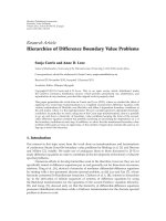
Figure 4.3.11:Educated at Queen’s College, Oxford, Clement John Tranter, CBE, (1909–
1991) excelled both as a researcher and educator, primarily at the Military College of
Science at Woolrich and then Shrivenham. His mathematical papers fall into two camps:
(a) the solution of boundary value problems by classical and transform methods and (b)
the solution of dual integral equations and series. He is equally well known for a series
of popular textbooks on integral transforms and Bessel functions. (Portrait provided by
kind permission of the Defense College of Management and Technology Library’s Heritage
Centre.)
What is thevalue of κ here? Clearly, we would like our solution to be
valid for a wide range of σ.Because G(λ) → 1asσ →∞,areasonable choice
is κ =1. Therefore, we take
sinh(k)A(k)=
∞

n=1

A
n
1+k coth(k)/σ
J
2n−1
(ka). (4.3.274)
Our final task remains to find A
n
.
We begin by writing
A
n
1+k coth(k)/σ
J
2n−1
(ka)=
∞

m=1
B
mn
J
2m−1
(ka), (4.3.275)
where B
mn
depends only on a and σ.Multiplying Equation 4.3.275 by dk/k ×
J
2p−1
(ka)andintegrating


∞
0
A
n
1+k coth(k)/σ
J
2n−1
(ka) J
2p−1
(ka)
dk
k
=

∞
0
∞

m=1
B
mn
J
2m−1
(ka) J
2p−1
(ka)
dk
k
. (4.3.276)

© 2008 by Taylor & Francis Group, LLC
250 Mixed Boundary Value Problems
Because
58

∞
0
J
2n−1
(ka) J
2p−1
(ka)
dk
k
=
δ
mp
2(2m −1)
, (4.3.277)
where δ
mp
is the Kronecker delta:
δ
mp
=

1,m= p,
0,m= p,
(4.3.278)
Equation 4.3.276 reduces to

A
n

∞
0
J
2n−1
(ka)J
2m−1
(ka)
1+k coth(k)/σ
dk
k
=
B
mn
2(2m −1)
. (4.3.279)
If we define
S
mn
=

∞
0
J
2n−1
(ka) J
2m−1
(ka)

1+k coth(k)/σ
dk
k
, (4.3.280)
then we can rewrite Equation 4.3.279 as
A
n
S
mn
=
B
mn
2(2m −1)
. (4.3.281)
Because
59
a

∞
0
J
0
(kr) J
2m−1
(ka) dk = P
m−1

1 −
2r
2

a
2

,r<a,(4.3.282)
where P
m
(·)istheLegendre polynomial of order m,Equation4.3.282canbe
rewritten
∞

n=1
∞

m=1
B
mn
P
m−1

1 −
2r
2
a
2

=1. (4.3.283)
Equation 4.3.283 follows from the substitution of Equation 4.3.274 into Equa-
tion 4.3.269 and then using Equation 4.3.282. Multiplying Equation 4.3.283
by P
m−1

(ξ) dξ,integrating between −1and 1, and using the orthogonality
properties of the Legendre polynomial, we have
∞

n=1
B
mn

1
−1
[P
m−1
(ξ)]
2
dξ =

1
−1
P
m−1
(ξ) dξ =

1
−1
P
0
(ξ)P
m−1
(ξ) dξ,
(4.3.284)

58
Gradshteyn and Ryzhik, op. cit., Formula 6.538.2.
59
Ibid., Formula 6.512.4.
© 2008 by Taylor & Francis Group, LLC
Transform Methods 251
Table 4.3.1:TheConvergence of the Coefficients A
n
Given by Equation
4.3.287 Where S
mn
Has Nonzero Values for 1 ≤ m, n ≤ N
NA
1
A
2
A
3
A
4
A
5
A
6
A
7
A
8
12.9980
23.1573 −1.7181

33.2084 −2.0329 1.5978
43.2300 −2.1562 1.9813 −1.4517
53.2411 −2.2174 2.1548 −1.8631 1.3347
63.2475 −2.2521 2.2495 −2.0670 1.7549 −1.2399
73.2515 −2.2738 2.3073 −2.1862 1.9770 −1.6597 1.1620
83.2542 −2.2882 2.3452 −2.2626 2.1133 −1.8925 1.5772 −1.0972
which shows that only m =1yieldsanontrivial sum. Thus,
∞

n=1
B
mn
=2(2m −1)
∞

n=1
A
n
S
mn
=0, 2 ≤ m, (4.3.285)
and
∞

n=1
B
1n
=2
∞


n=1
A
n
S
1n
=1, (4.3.286)
or
∞

n=1
S
mn
A
n
=
1
2
δ
m1
. (4.3.287)
Thus, we reduced the problem to the solution of an infinite number of linear
equations that yield A
n
.Selecting some maximum value for n and m,say
N,eachterminthematrixS
mn
,1≤ m, n ≤ N,isevaluatednumerically
for a givenvalue of a and σ.Byinverting Equation 4.3.287, we obtain the
coefficients A
n

for n =1, ,N.Because we solved a truncated version
of Equation 4.3.287, they will only be approximate. To find more accurate
values, we can increase N by 1and again invert Equation 4.3.287. In addition
to the new A
N+1
,theprevious coefficients will become more accurate. We
can repeat this process of increasing N until the coefficients converge to their
correct values. This is illustrated in Table 4.3.1 when σ = a =1.
Once we have computed the coefficients A
n
necessary for the desired ac-
curacy, we use Equation 4.3.274 to find A(k)andthenobtain u(r, z)from
Equation 4.3.268 via numerical integration. Figure 4.3.12 illustrates the solu-
tion when σ =1anda =2.
© 2008 by Taylor & Francis Group, LLC
Transform Methods 253
and
u
2
(r, z)=

∞
0
A(k)tanh(kb/a)e
kz/a
J
0
(kr/a)
dk
k

. (4.3.296)
Equation 4.3.295 satisfies not only Equation 4.3.288, but also Equation 4.3.290
and Equation 4.3.292. Similarly, Equation 4.3.296 satisfies not only Equation
4.3.289, but also Equation 4.3.291 and Equation 4.3.293. Substituting Equa-
tion 4.3.295 and Equation 4.3.296 into Equation 4.3.294, we obtain the dual
integral equations

∞
0
A(k)tanh(kb/a)J
0
(kr/a)
dk
k
=1, 0 ≤ r<a, (4.3.297)
and

∞
0
A(k)[1+
0
tanh(kb/a)/] J
0
(kr/a) dk =0,a<r<∞. (4.3.298)
If we define A(k)by
[1 + 
0
tanh(kb/a)/] A(k)=k

1

0
f(t)cos(kt) dt, (4.3.299)
then direct substitution of Equation 4.3.299 into Equation 4.3.298 shows that
it is satisfied identically. We next substitute Equation 4.3.299 into Equation
4.3.297 and interchange the order of integration. This yields

∞
0
tanh(kb/a)J
0
(kr/a)
1+
0
tanh(kb/a)/


1
0
f(t)cos(kt) dt

dk =1, 0 <t<1.
(4.3.300)
From Equation 1.4.9, we find that
d
dt


at
0
rJ

0
(kr)

t
2
− r
2
/a
2
dr

= a
2
cos(kt). (4.3.301)
Whydid we derive Equation 4.3.301? If we multiply both sides of Equation
4.3.300 by rdr/

t
2
− r
2
/a
2
,integratefrom0toat,differentiate with respect
to t,and useEquation 4.3.301, we obtain the following integral equation that
gives f(t):

1
0
f(τ)



∞
0
tanh(kb/a)
1+
0
tanh(kb/a)/
cos(kt)cos(kτ) dk

dτ =1; (4.3.302)
or,
π
2
f(t)−

1
0
f(τ)


∞
0
1 − tanh(kb/a)
1+
0
tanh(kb/a)/
cos(kt)cos(kτ) dk

dτ =


1+

0


,
(4.3.303)
© 2008 by Taylor & Francis Group, LLC
254 Mixed Boundary Value Problems
0
0.5
1
1.5
2
0
0.5
1
1.5
2
0
0.2
0.4
0.6
0.8
1
1.2
r/a
z/a
u

1
(r,z)
Figure 4.3.13:Thesolutionu
1
(r, z)tothe mixed boundary value problem governed by
Equation 4.3.288 through Equation 4.3.294 when  =3
0
.
if 0 <t<1.
At this point we mustsolveEquation 4.3.303 numerically to compute
f(t). Before we do that, there are two limiting cases of interest. When  = 
0
,
we have the same problem that we solved in Section 2.2 on the disc capacitor.
The second limit is 
0
 .Inthiscaseu
2
(r, z) → 0andu
1
(r, z)isgivenby
the solution to Example 4.3.2. Figure 4.3.13 shows the solution somewhere
between these two limits with  =3
0
.
• Example 4.3.14
During their study of a circular disk in a Brinkman medium, Feng et
al.
61
solved a system of mixed boundary value problems. We join their

problem midway in progress where they derived the following governing partial
differential equations and boundary conditions:
∂
2
u
1
∂r
2
+
1
r
∂u
1
∂r
−
∂
2
u
1
∂z
2
=0, 0 ≤ r<∞, −∞ <z<∞, (4.3.304)
∂
2
u
2
∂r
2
+
1

r
∂u
2
∂r
−
∂
2
u
2
∂z
2
−γ
2
u
2
=0, 0 ≤ r<∞, −∞ <z<∞, (4.3.305)
subject to the boundary conditions
lim
r→0
|u
1
(r, z)| < ∞, lim
r→∞
u
1
(r, z) → 0, −∞ <z<∞, (4.3.306)
61
Feng, J., P. Ganatos, and S. Weinbaum, 1998: The general motion of a circular disk
in a Brinkman medium. Phys. Fluids, 10, 2137–2146.
© 2008 by Taylor & Francis Group, LLC

Transform Methods 255
lim
r→0
|u
2
(r, z)| < ∞, lim
r→∞
u
2
(r, z) → 0, −∞ <z<∞, (4.3.307)
lim
|z|→∞
u
1
(r, z) → 0, 0 ≤ r<∞, (4.3.308)
lim
|z|→∞
u
2
(r, z) → 0, 0 ≤ r<∞, (4.3.309)
∂u
1
∂z
+
∂u
2
∂z





z=0
−
=
∂u
1
∂z
+
∂u
2
∂z




z=0
+
, (4.3.310)
and





∂u
1
∂r
+
∂u
2

∂r




z=0
−
=
∂u
1
∂r
+
∂u
2
∂r




z=0
+
= r, 0 ≤ r<1,
p(r, 0
−
)=p(r, 0
+
), 1 <r<∞,
(4.3.311)
where
∂p

∂z
= −
1
r
∂u
1
∂r
and
∂p
∂r
=
1
r
∂u
1
∂z
. (4.3.312)
Using Hankel transforms, the solutions to Equation 4.3.304 and Equation
4.3.305 are
u
1
(r, z)=

∞
0
A(k)e
−k|z|
rJ
1
(kr) dk, (4.3.313)

and
u
2
(r, z)=

∞
0
B(k)e
−|z|
√
k
2
+γ
2
rJ
1
(kr) dk. (4.3.314)
Equation 4.3.313 satisfies not only Equation 4.3.304, but also Equation 4.3.306
and Equation 4.3.308. Similarly, Equation 4.3.314 satisfies not only Equation
4.3.305, but also Equation 4.3.307 and Equation 4.3.309. Substituting Equa-
tion 4.3.313 and Equation 4.3.314 into Equation 4.3.310, we find that

∞
0

−kA(k) −

k
2
+ γ

2
B(k)

rJ
1
(kr) dk =0, 0 ≤ r<∞. (4.3.315)
Hence,
B(k)=−
kA(k)

k
2
+ γ
2
. (4.3.316)
Let us now turn to the equation involving p(r, z)inthe mixed boundary
condition Equation 4.3.311. Now,
∂p
∂z
= −
1
r

∞
0
A(k)e
−k|z|
d
dr
[rJ

1
(kr)] dk = k

∞
0
A(k)e
−k|z|
J
0
(kr) dk.
(4.3.317)
Therefore,
p(r, z)=f(r)+

∞
0
A(k)sgn(z)e
−k|z|
J
0
(kr) dk, (4.3.318)
© 2008 by Taylor & Francis Group, LLC