MOSFET MODELING FOR VLSI SIMULATION - Theory and Practice Episode 15 doc

SPICE Diode and MOSFET
11
Models
and Their Parameters
In this chapter we will discuss the pnjunction diode and MOSFET models,
as implemented in Berkeley SPICE2G and higher versions.
No
attempt
will be made to derive the model equations, as that has already been done
at appropriate places in previous chapters. Here we will only describe
equations used to model different regions of device operation. Emphasis
will be on model parameters required to run SPICE and how to measure
them.
Berkeley SPICE has four different MOSFET models of varying complexity
and accuracy [1]-[3]. These are (1) the Level
1
model-a first order model
suitable only for long channel devices;
(2)
the Level
2
model that includes
various second order effects present in small geometry devices, and is
considered to be a physical model;
(3)
the Level 3 model-a semi-empirical
model that includes most of the second order effects described in the Level
2
model;
(4)
the Level

4
model, called the BSIM (Berkeley Short-channel
Igfet Model), that
is
a
parameter based model. These different models can
be activated by a parameter called LEVEL. We will describe all four levels
of MOSFET model equations and their parameters. However, first we will
describe the diode model parameters and how to determine them.
11.1
Diode Model
The SPICE diode model has been discussed in detail in section 2.9.
Table
11.1
shows model parameters that determine both
DC
and
AC
characteristics of a diode.
Out of these ten parameters, the first seven
(Z,,
q,
r,,
Cjo,
4,
rn
and z) are
determined from diode drain current and capacitance measurements. The
remaining three parameters are often not measured and default values are
generally assumed for silicon

pn
junction diodes. For other type
of
diodes
such as SBD (Schotkey Barier Diode), parameter
XTZ
needs to be changed.
In
what follows we will discuss extraction for the first seven parameters.
11.1
Diode Model
537
Table
11.1.
SPICE Diode model parameters
Parameter SPICE
name in parameter Parameter
the text name description
Default
value Units
IS
XN
RS
CJO
PB
MJ
TT
BV
EG
XTI

saturation current
emission coefficient
series resistance
zero-bias junction capacitance
pn
junction potential
pn
grading coefficient
transit time
reverse breakdown voltage
band-gap voltage
IS
temperature exponent
1.10-l4
A
-
1
0
n
0
F
1
.o
V
0.5
0
sec
infinite
V
1.1

eV
3.0
-
-
These parameters are entered in the
MODEL
statement in the SPICE
input file.
Recall that
SPICE
calculates the diode current
I,
using the following
equation [cf.
Eq.
(2.82)]
I
d
-I
-
s[
exp
(
',;;"')
-
I]
which after rearranging in terms
of
V,
(voltage across the diode) becomes

(11.1)
where
I,,
rs
and
y
are model parameters that can be determined either
using linear regression methods, as discussed in section 9.14 or a nonlinear
optimization method (cf. Chapter
10).
In the latter case we
fit
the experi-
mental
I,
versus
V,
data to model equation (11.1) such that
(1
1.2)
is minimum, where
Vexp
and
Vca,
are the measured and calculated
V,,
respectively, and
1
is the number of data points. The result of this curve
fitting is shown in Figure 11.1 for a typical

n+p
diode fabricated using a
lpm
CMOS
process. The values for the parameter
I,,
q
and
r,
for two
types
of
diodes
(n'p
and
p'n)
are shown in Table 11.2. For comparison
the parameters obtained using the linear regression method (cf. section
10.14)
are also shown in this table.
Note that extracted parameter values from two different methods are not
exactly the same. However, for circuit simulation purposes, the parameter
538
11 SPICE Diode and
MOSFET
Models
s
-
10-4
u

10-5
3
10-6
0
U
z
U
U
0
I
%=
8.99
10-14
A
r,=
15.88R
n
=
1.19
10-9
1
)
1
o-’oo.o
0.5
1
.o
1.5
I
DIODE FORWARD VOLTAGE, Vd

(V)
Fig. 11.1 Plot
of
log(1,) versus
V,
for
a
n’p
diode. Circles are experimental points
while continuous line is nonlinear least-square lit to
Eq.
(1 1.1)
Table 11.2.
Diode parameters
I,,
n
and
R,
Linear Optimization Linear Optimization
regression method regression method
1,
4.53
x
10-l~~ 8.99
x
10-1~~
4.1
x
10-IZA 4.05
x

10-12A
v
1.119
1.19
1.335 1.346
R,
11.03R 15.88
R
10.78
R
14.27
R
set obtained using the optimization method is more appropriate, as these
values are obtained by fitting over all portion of the curve in the current
range
of
interest. Unlike the linear regression method, the optimization
method yields all three parameters simultaneously.
The parameters
Cjo,
4
and
m
describe the junction capacitance due to the
space charge in the junction depletion region. When the junction reverse
voltage
vd
is
less than
4/2,

the junction capacitance
Cj
is given by the
following equation [cf. Eq.
(2.74)]
(11.3)
where
Cjo
varies from device to device, but
is
typically of the order
of
1.0
x
pF/pn2. The barrier potential
4
is usually about
0.5-0.7
V
and
the gradient factor
m
is assumed to be between
0.333
(linearly graded
11.1
Diode
Model
539
junction) and 0.5 (abrupt junction), although values outside this range are

not uncommon.
The parameters
4
and
m
are generally determined by curve fitting
Eq.
(1
1.3)
with measured data using a nonlinear least square optimization program.
Very often,
Cjo
is also treated as a parameter to be optimized along with
4
and
m
rather than taking its value from measured data. This is because
3
parameters
(Cjo,
4
and
m)
when optimized together give better fit over
the entire data range
of
interest (see Figure 2.19 and Table 9.4).
Transient Time
z,.
The parameter

z,
is the diode transit time and
is
used
to calculate the diode diffusion capacitance
C,,
[cf. Eq.
(2.77)]
when the
diode is forward biased. Typical values
of
z,
range from 1 to 100 nsec.
There are different electrical methods
to
calculate transit time
z,,
like the
voltage decay method, the reverse recovery method, etc [4]. However, the
simplest method of obtaining
z,
is to compute it from the reverse recovery
method. In this method, we measure the diode storage time
t,
by switching
the diode from a forward voltage
V’
to a reverse voltage
V,,
and using the

following equation [4]-[6]

(11.4)
where
I,
and
I,
are the forward and reverse current, respectively, when the
diode is switched from the forward voltage
V,
to the reverse voltage
V,.
Note that this equation requires evaluation of the error function, which is
approximately given by [4]
erf(x)
=
~
exp
(-
z2)dz
ho
S’
Due to the complexity of Eq. (1 1.4), the Newton-Raphson method is needed
to compute
Z,
and is thus fairly involved. However, the following simple
equation
is often used to calculate
z,
t,

=
zr
[
In
(1
+
91.
(11.6)
As
shown in Figure 11.2, there is a discrepancy
of
30%
between the
z,
calculated using
Eqs.
(11.4) and (11.6) even when
I,
>>
I,.
Therefore, it is
advisable to
use
Eq. (11.4). While using
Eq.
(11.6), it has been suggested
that
IJ>>Z,
must
be

kept in the measurements. This way, the affect of
540
11 SPICE Diode and MOSFET Models
Fig. 11.2 Plot
of
tJtt
versus
IJ/Ir
using Eq. (11.4) (continuous line) and (11.6) (dotted
line). Continuous line predicts more exact value
of
z,
n+
p
diode
t
250.0
10.
0.0
I
1.0
1
+
Ir
/If
Fig. 11.3 Plot
of
t,
versus (1
+

If/I,)
for
a
n'p
diode using
Eq.
(11.6). Circles are
experimental points while continuous line
is
linear regression
of
Eq.
(11.6)
recombination in the heavily doped region is entirely eliminated
[4].
Under
these conditions, the plot
of
t,
versus ln(1
+
If/Ir)
will be a straight line
(see Figure
11.3)
the slope
of
which gives
7,.
The plot will be highly curved

if the condition
I,
>>
I,
is not met and then a unique value
of
lifetime
can
no
longer be extracted.
11.1
Diode Model
I
___
-
8V
I
11
\I
I
-3v
I
I
54
1
I
-T_Lr
INPUT
SIGNAL
I._.

-;
c-xc
(CH.l)


,
I
__.
-
_.~__I
HP
5Llll
D
OSCILLOSCOPE
HP
7550A
PLOTTER
-
-
-
-
-
-
-
-
-
-
Fig.
11.4
Test setup

for
measuring storage time using reverse recovery method
Equipment required for measuring
z,
are
(1)
a fast pulse generator such as
an HP8116A,
(2)
a fast oscilloscope, such as a Tektronix 7854 or an
HP54111D with dual trace plug-in, and
(3)
an
X-Y
recorder (optional). The
advantage
of
the HP8116A function generator is that it can supply an asym-
metric pulse waveforms. However, if not available, two pulse generators
are needed to adjust the voltages
Vr
and
V,
independently. The test configu-
ration
is
shown in Figure 11.4. The time delay due to connectors and series
resistance in the circuit should be carefully minimized. The resistor
R,
(350

a)
is chosen such that the DC current flowing into the diode is limited
within the range of
f
15
mA for voltages between
Vr
=.
8
V
(forward bias)
and
V,
=
-
3
V
(reverse bias) and the RC delay time introduced by this
resistor is negligible as compared to the diode transit time.
During forward bias (at
t
=
0-),
a positive voltage
(Vs
=
8
V)
at
f=

100
Hz
was applied to the circuit. The current was then calculated by dividing the
Fig.
11.5
Storage time
t,
as
a
function
of
input pulse
for
n'p
diode
542
1
I
SPICE
Diode and MOSFET Models
Table
11.3.
Diode
transit
time
t,
calculation using nS nS
Error
function
Eq.

(1
1.4)
241.3
415
Transit time
nip
P+n
Log
function
Eq.
(1
1.6)
-
339
voltage measured
on
resistor
R,
(50
0).
At
t
=
0,
a negative voltage is applied
to the diode; the input pulse changes from
+
8 V
to
-

3
V
at
t
=
0.
The
diode storage time was measured as the time from beginning of the
reverse current transition to the time when the reverse current begins to
decay toward its leakage current value (see Figure
11.5).
The lifetime
z
calculated using the above method for both
n+p
and
p+n
diodes are shown in Table
11.3.
Note the difference between
z,
calculated
using Eqs.
(1
1.4) and
(1 1.6).
11.2
MOSFET
Level
1

Model
The level
1
model is often referred to as the Shichman-Hodges model. It
is the simplest of the four MOSFET models in
SPICE
and is
accurate
onZy
for
long
channel
devices.
11.2.1
DC
Model
The threshold voltage
Vth
for the SPICE Level 1 model is [cf. Eq. (5.16)]
(11.7)
where
V,,
is the zero-bias
(V,,
=
0
V)
threshold voltage
of
a long channel

device,
y
is the body factor, and
+f
is
the bulk Fermi potential. Note that
no short channel
or
narrow width effects are taken into account; for details
see
section
5.1.
The saturation voltage
V,,,,
is calculated using the following equation
[cf. Eq. (6.54)]
(11.8)
The drain current
I,,
is calculated using the following relations [cf.
Eq. (6.62)]
S,[(Vg,-
Kh-+vdS)Vds](1
+A&,)
linear region,
Vgs
>
I/,,and
v,,~
v,,,,

Ids=
0.5PO(Vgs
-
vth)2(1
+
nvds)
saturation region,
V,,
>
V,,,,
subthreshold region,
V,,
I
V,,
vdsat
=
vgs
-
Kh.
(11.9)
I0
where
Po
=
K(
W/L)
and
K
=
poco,.

11.2
MOSFET
Level
1
Model
543
Note that the channel length modulation factor,
I,
is included in both the
linear and saturation regions,
so as to make the current and its first
derivative continuous,
as
was explained in section 6.4.1. Also note that the
subthreshold current is zero.
In addition to the intrinsic MOSFET DC current equations described
above, one needs
to
model the source/drain (S/D)-to-substrate
pn
junctions.
Since in the normal operation of the device these junctions are reverse
biased, the only DC parameter of the S/D junction which is of interest is
the saturation (leakage) current
I,.
In SPICE this is specified as
J,,
the
saturation current per unit area, or
I,,

the total saturation current. If
J,
is
specified then one needs to specify the source and drain areas
A,
and
Ad,
respectively.
11.2.2
Capacitance Model
The parameters
of
the dynamic model are the source/drain junction
capacitances, the overlap capacitances, and the intrinsic MOSFET capaci-
tances. The junction capacitances are the sum of both the bottom-wall
(area) capacitance and side-wall (periphery) capacitance. The source diode
capacitance
C,,
is computed
as
follows [cf. Eq. (3.26)]
(11.10)
where
A,
and
P,
are the area and periphery
of
the source-to-bulk
pn

junction,
respectively, and
Cjo and
Cjswo
are the junction capacitance per unit area
and per unit periphery, respectively, at zero back bias.
A
similar equation
holds for the drain-to-bulk junction capacitance
CBD.
These equations are
used
for
all SPICE models.
The intrinsic device capacitances (also sometimes referred to as gate oxide
capacitances) are based on the Meyer model (see section 7.1.1). There are
only three intrinsic capacitances
C,,,
C,,
and
CGB
in the Meyer model.
Their values change with bias conditions as follows:
Strong Inuersion Region.
In the strong inversion region when V,,
>
Vth, the
gate capacitance is calculated using the following relations:
Linear
Region:

In this case
Vgs
>
(vth
+
Vd,)
(1
1.1 la)
(1 1.1 1 b)
(1 1.1 lc)
c,,
=
0.
544
11
SPICE
Diode
and
MOSFET
Models
Saturation Region:
In this case
V,h
<
V,,
<
(V,h
+
V&)
c,,

=
3
2
cox,
(11.12a)
c,D
=
0
(1 1.12b)
c,,
=
0
(1
1.12c)
cox,
=
WLC,,.
(1
1.12d)
Weak Inversion Region.
In SPICE this region, defined as
V,,
<
I/th,
is
divided into two parts. For the sake of simplicity the transition between
the saturation and weak inversion regions is made linear, resulting in the
following equations.
where
When

(vih
-
4f)
<
vgs
<
I/th?
(11.13a)
c,,
=
0
(1 1.1
3b)
(11.13~)
(1 1.14a)
(1 1.14b)
(1 1.14~)
Note that these capacitances do not require any new parameters.
The overlap capacitances
C,,,, CGD0
and
C,,,
are then added to
C,,, CGD
and
C,,,
respectively, in different regions
of
device operation and are
calculated from the following equations:

c,,,
=
c,sow
(
1
1.1
5a)
cGDO
=
Cgdo
(1
1.15b)
CGBO
=
CgboL.
(11.15~)
Normally
Cgso
=
Cgdo,
the overlap capacitance per unit width at the source
and drain ends, respectively. The model parameters for the SPICE Level 1
model are shown in Table 11.4. These parameters are entered in the
MODEL
statement in the SPICE input file.
In addition to the model parameters shown in Table 11.4, the
device
parameters
shown in Table 11.5 are also required. These device parameters
546

11
SPICE Diode and MOSFET Models
Table
11.5.
Device parameters
Parameter SPICE
name in parameter Parameter Default
the text name description value Units
L,
L
Drawn Channel length (mask dimensions) m
wm
W
Drawn Channel width (mask dimensions) m
AS
Source diffusion area
0.0
m2
As
Ad
AD
Drain diffusion area
0.0
m2
PS Perimeter
of
the source diffusion window
0.0
m
ps

Pd
PD
Perimeter
of
the drain diffusion window
0.0
m
-
NRS
Number
of
squares in the source diffusion
1.0
m
~
NRD
Number
of
squares in the drain diffusion
1.0
~
electrical parameters will always override the value computed from
process parameters, if also specified. Thus, if
VTO,
NSUB
and
TOX
are
input, the threshold voltage will assume the value entered as
VTO,

while
GAMMA
will be computed from
NSUB
and
TOX.
Similarly, if
KP
is
not specified but
UO
is specified, then
KP
will be computed using either
the specified value of
TOX
or its default value, if not specified.
If
VTO
is not an input parameter then one needs to specify
NSUB,
TOX
and
TPG,
which are then used to calculate
V,,
using
Eq.
(5.15).
The last parameter

TPG
denotes the type of the gate and can take any
of the following three values
+
1
for gate type opposite to the substrate
TPG
=
-
1
for gate type same as the substrate (11.16)
and is used to calculate
Qms
and hence
V,,(=
Qms-
qN,,/C,,)
[cf.
Eq.
(4.14)], as follows:
I
0
for aluminum gate
-
0.5
-
0.5E,
-
0.54, for TPG
=

0
forTPG= -1
where
E,
is the energy gap for silicon [cf.
Eq.
(2.3)].
SPICE
sets all parameters to the default values if negative values are
input by the user, with the exception of
VTO, TPG
and
NSS.
Thus, if
GAMMA
is specified as a negative value, then
SPICE
assumes it to be
zero, which is the default value.
0
For a p-channel enhancement and an n-channel depletion device
VTO
is negative, while it is positive for n-channel enhancement devices. Recall
that p-channel depletion devices are not fabricated, but if simulated, their
VTO will be positive.
Qms
=
-
0.5E,
-

0.54, for
TPG
=
1 (11.17)
1
0.5E,
-
0.54,
11.2
MOSFET
Level
1
Model
541
0
The default value
of
TOX
=
lo-’
m
(1000
A)
is valid for the Level
2
and
higher level models. If
TOX
is not specified
for

LEVEL
=
1,
then
TOX
acts as
a
flag and “turns
off”
the use of process parameters resulting in
the omission
of
intrinsic capacitance calculations.
0
The parameter LAMBDA in the Level
1
model defaults to zero if it
is not specified. However, this is not the case in the Level
2
model as
we will see later.
Some parameters in the model may be specified in more than one way.
For
example, reverse or saturation current of the junction can be specified
either as
IS
or
JS.
Whereas the first is an absolute value, the second is
multiplied by

AS
and
AD
to give the saturation current
of
the source
and drain junctions, respectively. However, the advantage of specifying
JS
is that the resulting value of the saturation current becomes specific
to each junction
of
each transistor; unlike giving
IS,
which will result in
the same value
of
the saturation current for all sourceldrain junctions.
Similarly, the zero-bias depletion capacitances can be specified by
CJ,
which is multiplied by
AS
and
AD,
and by
CJSW
which is multiplied by
PS
and
PD
specific to each single device. Or, they can be set by

CBD
and
CBS,
which are absolute values.
The parasitic ohmic resistances of the source and drain junctions can be
specified either by
RD
and
RS
which are the absolute values, or by
RSH
which is multiplied by
NRS
and
NRD.
If
both
IS
and
JS
are specified,
IS
overrides
JS.
Model
Parameter Determination.
Determination of all Level
1
parameters,
except that

of
K
(KP) and
2
(LAMBDA) have been discussed earlier. The
parameter LAMBDA is
a
saturation region parameter and can be
determined from the slope of the
Id,
versus
vd,
curve in the saturation region
(V,,
>
Vd,,,)
by dividing the slope value by the y-intercept. The slope in the
saturation region is very small, and therefore care must be exercised in its
determination. The parameter
KP
can be determined either from the slope
of the linear region plot
of
Id,
versus
Vgs
at low
Vd,
or from the slope of
JIds

versus
V,,
curve with
I,,
obtained in the saturation region.
For
a typical 2pm CMOS technology, the value of KP obtained from linear
region data is
27
pA/V2, while the corresponding value obtained in
saturation is 22pA/V2. Clearly, the value of KP obtained from the two
methods is different because the mobility degradation due to the gate field
is not taken into account in this model. Since SPICE allows only one value
to be used for both linear and saturation regions, it is more appropriate to
use an optimizer to extract KP along with other parameters.
548
11
SPICE
Diode
and
MOSFET
Models
11.3
MOSFET Level
2
Model
The Level 2 model incorporates many of the second order effects
for
small
size devices. It can model

a
reasonable range
of
device sizes,
but
is
computationally quite complex.
11.3.1
DC
Model
The threshold voltage equation for the SPICE Level 2 model
is
'rh
=
VTo
-
Y&
+
?/FIJm
+
Fw(24f
+
'sb)
(1
1.18)
where
F,
is
the short channel factor based
on

Yau's modified model
as
given by
Eq.
(5.94) and
Fw
is the narrow width factor based on
a
simplified
thick field oxide model [cf. Eq.
(5.91)]
given by
(11.19)
Linear Region Current.
The drain current in the linear region is given by
zds=Ijeff[('gs-
v,*,-~r]V~s)'~s-~?/Fl{(V~s
+
2df
+
Vsb)3i2
-
(24f
+
'sb)3i2
11
(11.20)
where
(1 1.21a)
(1 1.2 lc)

y=l+Fw
(
1
1.2
1
d)
(1 1.21e)
(11.21f)
and
L,
is
the drawn channel length, while
Ldif
is the side diffusion [cf.
Eq.
(3.31)]. Note that the channel length modulation (CLM) factor
/z
is
used for both linear and saturation regions of device operation,
so as
to
make the current and its first derivative continuous from linear to saturation
region, as was explained in Chapter
6.
Saturation Voltage.
The saturation voltage
V,,,,
is calculated in one
of
two

ways. If the maximum carrier drift velocity
u,,,
is assumed zero, then
V,,,,
549
11.3
MOSFET
Level
2
Model
is calculated Using
a
pinch-off model (i.e.,
Ids/I/ds
=
0
at
Vds
=
Vdsa,,
as
discussed
in
section
6.4.1),
otherwise
it
is
calculated using the velocity
saturation model.

Vdsat
using the
pinch-off model:
In this case
VdSa[
is
calculated from the
following equation:
where
'sb)]'"]
(11.22)
Vdsaf
using
the velocity saturation model:
In this case
I/dsat
is calculated
using the Baun and Benking model from the following equation [cf.
Eq. (6.173)]
where
(1
1.23)
Note that in order to solve for
vd,,,
one needs to know
Leff.
This means
that
vd,,,
calculations requires simultaneous solution of two nonlinear

Eqs.
(1
1.25) and
(1
1.21e). However, SPICE uses the following closed form
solution by making the approximation that
Leff
=
L in
Eq.
(1 1.25). With
this approximation one can write Eq. (11.25) in
a
somewhat more manage-
able form, if the following substitutions are made
(1 1.26a)
550
11
SPICE
Diode
and
MOSFET
Models
(1
1.26~)
(1 1.26d)
With this substitution, Eq.
(1
1.25) becomes:
(1

1.27)
It is clear that the above equation can be written
as
a
fourth order
polynomial equation in
X
as:
(11.28)
(V,
-
$V2
-
iX2)(X2
-
V2)
-
+(yFJq)(X3
-
Vi’2)
U=
Vl
-
(YFl/rl)X
-
x2
X4
+
AX3
+

BX2
+
CX
+
D
=
0
where the coefficients
A,
B,
C
and
D
are:
B
=
-
2(V1
+
u)
YFl
c=
-2 0
rl
4
YF
3rl
D
=
2V1(V2

+
U)
-
V;
I
V;”.
Equation (11.27) is solved for
X
using a closed form method known as
Ferrari’s method. Once
X
is known, it is a trivial matter to obtain
Vd,,,
from Eq. (11.26d). Since Eq. (11.27) is
a
fourth order polynomial equation,
it has four possible solutions. The smallest positive solution is taken to be
the valid solution. If no positive real roots are obtained, then
vd,,,
is
evaluated using the pinch-off model, Eq.
(1
1.22).
Leff
Calculation.
The
Leff
is calculated using Eq. (11.21e)
Leff
=

L(l
-
.2vds)
(11.29)
and depends upon whether or not the
CLM
term
il
has a finite value. If
.2
=
0
is input to the model parameter file, then channel length modulation
is not taken into account and
Leff
=
L. However, if
1
is not input then it
is calculated internally. Depending upon the value of
urnax,
il
is calculated
from either of the following two equations:
If
u,,,
20,
V,,,,
is calculated using the pinch-off model,
Eq.

(11.22),
while the effective channel length is evaluated using the following
11.3
MOSFET
Level
2
Model
551
equation:
(11.30)
If
u,,,
>
0,
then
Vdsa,
is
calculated using
Eq.
(11.26d), and
A
is
given
by
I
=
qJ(+)2
+
(V,,
-

V,,,,)
-
vds
(11.31)
Note that
X,
used in
Eqs.
(11.30) and
(1
1.31) are different. This is because
Eq.
(1 1.30) does not provide an accurate description
of
the output
conductance in saturation and
Neff
has to be used as
an
empirical factor
to change the substrate doping
to
NeffNb.
The larger the
Neff,
the smaller
the output conductance becomes. The range of
Neff
is
normally between

1
and
5.
Saturatioiz
Region Current.
In this region,
V,,
>
v&,,
and current is calculated
using
Eq.
(11.20)
with
VdS
replaced by
Vdsat.
Subthreshold
Current.
The
current in the subthreshold region
is
calculated
using the following equation:
(1
1.32)
where
kT
4
v,,

=
v,,
+
n-
and
lo
is
the value
of
I,,
at
Vgs
=
V,,
calculated using
Eq.
(1
1.20),
N,,
is a
curve fitting parameter and
C,
is
the depletion capacitance. The voltage
V,,
makes the transition from weak to strong inversion regions.
The
DC
parameters for Level
2

model are shown in Table 11.6.
In
this
table
only
those parameters are included which are
in
addition to the Level
1
parameters shown in Table 11.4.
552
11
SPICE
Diode and
MOSFET
Models
Table
11.6.
SPICE
Level
2
model parameters. These are in addition
to
those shown in
Table
I I
.4
Parameter SPICE
name in parameter Parameter
the text name description

Default
value Units
Level
Ldif
LD
DELTA
XJ
UCRIT
UTRA
UEXP
VMAX
NEFF
NFS
XQC
Lateral diffusion
Narrow width factor
Junction Depth
Critical field for mobility degradation
Mobility transverse field coefficient
Exponent in mobility degradation
Maximum carrier drift velocity
Effective substrate doping factor
Fast surface state density
Thin-gate oxide capacitance model
flag and coefficient of channel charge
share attributed to drain
(0-0.5)
1
0.0
0.0

0.0
0.0
0.0
0.0
1
0.0
1
.0
1.104
Note the following:
The parameter
LD
accounts for the diffusion effects in the device length
direction giving an effective channel length
L
as
L
=
L,
-
2Ldi,.
The
UC
Berkeley implementation of the Level
2
model
does
not
have the parameter
WD(

=
AW)
for calculating the effective device width
from drawn dimensions resulting in
W,
=
W.
The parameter
UTRA
(cf. Eq. 11.21~) does not exist in the Berkeley
version, but it is included here because it exists in most of the Level
2
models in commercially available implementations
of
SPICE.
If
XJ
is not specified, the narrow channel effect is neglected.
If
NFS
is not specified, the subthreshold current is not calculated.
If
NFS
is not specified,
Vo,
=
Vth.
If
VMAX
is not specified, the velocity saturation effect is neglected.

11.3.2
Capacitance
Model
The MOSFET source and drain junction capacitance models are the
same as for Level
1.
However, for MOSFET intrinsic capacitances there
are two models available. The first model, which
is
also the default model,
is the Meyer model as described for Level
1;
the only difference being that
Fh
is replaced by
Van.
The second model is the charge controlled model
of
Ward and Dutton
[9].
The parameter
XQC
is associated with partioning
11.3
MOSFET Level
2
Model
553
Table
11.7

Charge sharing for Level
2
capacitance
model
Source Charge
Qs
Drain Charge
QD
Linear Region
QiP
QiP
Saturation Region
XQC’QI
(1
-
XQCIQi
of
the charge (see section
7.2).
In the Level
2
model the following scheme
is used to partition the channel charge
QI
into the source and drain charges,
Qs
and
QD,
respectively, (see Table 11.7). The
XQC

2
0.5
is user input
model parameter and indicates portion of the charge attributed to the
drain. It also acts as a
flag;
XQC
=
1
invokes the Meyer model. The parti-
tioning scheme causes discontinuity at the boundary
of
the linear and
saturation regions, except when
XQC
=
0.5.
Note that when
XQC
=
1,
then
in saturation
QD
=
0.
Model Parameter Determination.
The parameters of this model may be
divided into two parts; (1) basic parameters which are basically long channel
model parameters like VTO,

KP,
GAMMA
and
PHI
and
(2)
parameters
relative to second order effect not included in the basic model, and describe
narrow and short channel behavior. We have already discussed parameters
in the first part which are linear region parameters extracted using linear
regression methods. However, the linear regression method to calculate the
saturation region parameters, such as
VMAX,
or short-channel and narrow-
width parameters, are not straight forward. It is best to determine these
second order parameters using an optimizer as discussed in Chapter
10.
The presence of the parameter
NFS
permits calculation
of
the subthreshold
current in the model. The parameter can be calculated using
Eq.
(6.102)
and
(6.11
3). For long channel device
(11.33)
where

S
is the subthreshold slope. The parameters
y
and
4f
need to be
known and can be determined from
V,,
versus
V,,
measurements. The
extracted value is normally very high
(Nfs
=
9.3
x
10”
cm-*), although fast
surface states for the process are less than 10’0cmp2. The NFS is treated
simply as a fitting parameter. This model does not insure good correlation
with measurements.
The Level
2
model, though physically based, has various drawbacks. For
example, the transition from linear to saturation regions is not smooth,
particularly for short-channel devices, and there is
a
small discontinuity in
the transition from subthreshold to saturation region.
554

11
SPICE Diode
and
MOSFET Models
11.4
MOSFET
Level
3
Model
The Level 3 is a semi-empirical model that includes second order effects
due to short-channels and narrow-widths. The model is computationally
efficient compared to the Level
2
model, but the empirical model parameters
become geometry dependent.
11.4.1
DC
Model
The threshold voltage equation for the
SPICE
Level
3
model is
‘th
=
‘To
-
+
YFIdm
+

Fw(24f
+
‘sb)
-
gvds
(11.34)
where
F,
is a short channel factor based on Dang’s model, as given by
Eq.
(5.73),
F,
is a narrow width factor as in Level
2,
except that the
factor
of
4 is replaced by
2,
and
CT
is the
DIBL
parameter given by [cf.
Eq.
(5.106)
]
8.15.10-
22yl
Is=

C0J3
’
Linear Region Current.
The drain current,
Ids,
in the linear region is given
by [cf.
Eq.
(6.169)]
Ids
=
P(
‘qs
-
‘th
-
3‘
‘ds)
‘ds
(1
1.35)
where
(1
1.36a)
( 1 1.36b)
Ps
=
Pam +
Q(‘,,
-

‘tJ1
a=l+
(1 1.36~)
+
F,.
(
1
1.36d)
YFI
4JW
If
the parameter
omax
is
not specified by the user, peff
is
set to
ps
and the
velocity saturation effect is not modeled.
11.4
MOSFET
Level
3
Model
555
Saturation Voltage.
VdSat
is calculated from one of the following equations
(see section

6.7.2)
(if
u,,,
specified)
a
PS
(if
umax
not specified).
vgs
-
Vh
a
vdsat
=
(1 1.37)
Saturation Region Current.
Id,
in the saturation region is calculated Using
the following equation
(11.38)
where
€,=-
Idsat
GdsatL
(11.39b)
(11.39~)
dI*sat
(1
1.39d)

and
Idsat
is the drain current at saturation obtained by replacing
V,,
with
VdSat
in
Eq.
(11.35) and
Gdsat
is the drain conductance at saturation. The
fitting parameter accounts for the fact that the voltage across the depleted
surface of the channel, of length
l,,
is less than
V,,
-
V,,,,.
Gdsat
=
___
d
Vd,,,
Subthreshold Region Current.
It
is
given by the same equation as for the
Level
2
model [cf. Eq. (11.32)] except that

I,
now is calculated at
V,,
=
V,,
using
Eq.
(11.35).
The
SPICE
Level 3
DC
model parameters are shown in Table 11.8. These
parameters are in addition to the Level
1
parameters shown in Table 11.4,
except for the parameter
LAMBDA,
which is not used in Level 3.
The model parameters are generally extracted using an optimizer. Often
the value of
VMAX
is 3-5 times higher than the physical value. To get a
more realistic value, it has been suggested [13] to introduce one more
556
11
SPICE Diode and MOSFET Models
Table
11.8.
SPICE

Level
3
model parameters. These are in addition to those shown in
Table
11.4
Parameter
SPICE
name in parameter Parameter Default
the text name description value Units
Level
Liff
LD
G,
DELTA
XJ
NFS
X
j
Nrs
0
THETA
I
ETA
x
KAPPA
vlnax
VMAX
Lateral diffusion
Narrow width factor
Junction Depth

Fast surface state density
Mobility degradation factor
Static feedback factor
Saturation field correlation factor
Maximum carrier drift velocity
I
0.0
0.0
m
0.0
cm-*
0.0
V-'
0.0
0.2
~
-
-
~
empirical parameter DEL,
so
that
Eq.
(1 1.36b) reads
(11.40)
Usually, the value of this parameter is less than one. Note that unlike
VMAX
of the Level
2
model, the

VMAX
parameter in level 3
is
used in a
very different form and is fairly easy to extract from a linear regression
method.
The capacitance model (intrinsic and extrinsic)
is
the same as level
1
model.
11.5
MOSFET Level
4
Model
The
MOSFET
Level 4 model is generally known as
BSIM
and
is
in fact
a modified form of
CSIM
(Compact Short-channel Igfet Model)
[2].
This
is a parameter based model whose parameters are generally extracted
using automated extraction procedures using linear regression
[

101.
Since
the model has many parameters which are bias dependent, care must
be taken in extracting these parameters.
11
S.1
DC
Model
In this model, threshold voltage is expressed as [cf.
Eq.
(5.46) and (5.96)]
yh
=
vJb
+
24f
+
YJm
+
Kl(24f
+
vsb)
-
Ovds.
(11.41)
11.5
MOSFET
Level
4
Model

551
Linear and Saturation Region Current.
In these regions current is given by
&ff[(V,s
-
Vth
-
+ctI/ds)V&]
p(Vgs
-
Vth)2
linear region,
v,,
>
v,,
saturation region,
Vd,
>
Vds,,
Ids
=
p1
(11.42)
i
2ctK
where
(1 1.43a)
(11.43b)
(1 1.43~)
1.

(11.43d)
a=
1
+
[l-
1
2Jm
1.744
+
0.8364(24,
+
Vsb)
Note that the parameter
Uo
is
the same as 8 of Eq. (11.35) for Level 3.
The saturation voltage
Vds,,
is
calculated using the following equation.
where
K=+(l+
Vc+J1+21/,)
(11.44)
(11.45a)
(1
1.45b)
Subthreshold Region Current.
The subthreshold current is calculated using
the following equation

[8]
(11.46)
1'
=
lsub'dl
sub
'sub
+
Id1
where
Po
w
Id,
=
(3Vt)2.
2L
(11.47b)
558
11
SPICE
Diode
and MOSFET Models
The factor is empirically chosen to achieve the
best
fit in the
subthreshold characteristics with minimum effect
on
the strong inversion
characteristics.
The above model has only

9
basic parameters,
5
for threshold voltage
(V,,,
df,
y,
K,
and
v])
and 4 for drain current
(Po,
Uo,
U,
and
n).
However,
5
parameters
(v],
Po,
Uo,
U,
and
n)
depend on bias voltages
Vd,
and
V,,
as

follows:
(1 1.48a)
(11.48b)
(1 1.48~)
(1 1.48d)
and
po
(or
Po)
is modeled by quadratic interpolation through
3
data points:
po
at
vd,
=
0,
po
at
vd,
=
vdd
and the slope of
po
with respect to
Vd,
at
Vd,
=
Vdd

and can be expressed as
uO
=
uOz
+
uObvbs
ul
=
ulz
+
ulbVbs+
uld(vds
-
‘dd)
v]1
=
v]lz
+
v]lbvbs
+
v]ld(Vds
-
vdd)
n1
=
110
+
nbI/bs
+
ndVd/ds

where
(1 1.48e)
(1 1.49a)
(11.49b)
(11.49~)
where
vdd
is the drain voltage at which saturation region measurements
are made. Thus, there are total of
20
electrical parameters including
3
subthreshold region parameters
(no,
nb
and
nd).
These electrical parameters
also have length and width dependence. The sensitivity of a parameter to
L
(effective channel length) and
W
(effective channel width) is denoted by
adding a letter
‘L‘
and
‘W’
at the start of the parameter name. For example,
vfb
is a basic parameter with units of volts, and

LVFB
and WVFB are
parameters which accounts for length and widths dependence
of
VFB;
that
is,
LVFB
and
WVFB
are the corresponding L and
W
sensitiuityfuctors
for
VFB
and have units of Volts.pm. In general a parameter
Pi,
which has
length and width dependence, is expressed as
p,
pw
Pi
=
Po
+-
+

LW
(1
1

SO)
11.6
Comparison
of
the Four MOSFET Models
559
Table
11.9.
SPICE
Level
4
model parameters
Parameter SPICE
name in parameter Parameter
the text name description
Units
VFB
PHI
K1
K2
ETA
X2E
X3E
uo
X2UO
u1
x2u
1
X3U1
MU2

X2MZ
MUS
XZMS
X3MS
NO
NB
ND
DL
DW
TOX
Flat band voltage
Surface potential in strong inversion
Body factor
S/D
depletion charge sharing coefficient
Zero-bias DIBL coefficient
Sens.
of
DIBL effect to
Vb,
Sens.
of
DIBL effect to
Vd,
at
vd,
=
Vdd
Zero-bias trans. field mobility degradation
Sens. of trans. field mobility degradation

Zero-bias velocity saturation coeff.
Sens. of velocity saturation effect to
Vb,
Sens.
of
velocity saturation effect to
Zero-bias mobility
Sens.
of
mobility to
V,,
at
Vd,
=
0
Mobility at
Vb,
=
0
and at
V,,
=
Vdd
Sens.
of
mobility to
V,,
at
Vds
=

0
Sens.
of
mobility to
Vd,
at
Vda
=
vdd
Zero-bias subthreshold slope coefficient
Sens. of subthreshold slope to substrate
Sens. of subthreshold
slope
to drain bias
channel shortening
channel narrowing
Gate oxide thickness
effect to substrate bias
vds
at
vds
=
vdd
bias
XPART Channel charge sharing coefficient
11
S.2
Capacitance
Model
The source/drain junction capacitance model is the same as in Level

1
model but the
MOSFET
intrinsic capacitance model is a charge based
model. The parameter
XPART
is associated with partitioning of the
channel charge into drain and source components.
XPART
=
0
selects
60/40
partition of the channel charge to the source and drain, respectively,
while
XPART
=
1
sets
100/0
partition in the source/drain charge in satura:
tion. Parameters for the SPICE Level
4
model are shown in Table
11.9.
11.6
Comparison of
the
Four
MOSFET

Models
As
was stated earlier, the Level
1
model is useful only for hand calculations
and rough estimate of the circuit performance. The Level
2
model is more
physical compared to the Level
3
model. However, Level
2
model often
560
11
SPICE
Diode
and
MOSFET Models
causes convergence problems, and also takes
25%
more
CPU
time, compared
to Level 3 model, for each model evaluation. In this respect the Level 3
model is preferable. Because
of
the physical nature
of
the Level

2
model,
it is still used in spite
of
its drawbacks. Modifications to the Level
2
model
have recently been proposed. The Level 4 model is based on the physics
of the device. However, it has a large number of length and width dependent
parameters, and therefore, requires large number
of
devices to extract the
parameters.
Performance comparison of the four models have been reported recently
with the aim to see how different models scale with the device length and
width. For this comparison, n-channel MOSFETs ranging in masked
channel length (L,) and width
(W,)
from 10.4 to 1.4pm were characterized
[12]. Three different size devices were used to extract the model parameters
for Levels 1-3, while six WILdevices were used in order to get 34 length
and width dependent parameters for Level 4. A nonlinear optimization
method was used to determine the parameters. The channel length reduction
parameter LD (due to processing effect) was about 0.35pm, and channel
width reduction parameter
WD
was
0.55
pm, resulting in an effective
minimum geometry device

of
0.3 by 0.7pm. Although Levels 1-3 do not
have a
A
W
parameter, the parameter extraction was carried out using an
effective device width obtained by subtracting the known
AW
from the
drawn width.
First, the basic parameters
(MUO,
VTO,
GAMMA,
NSUB)
and mobility
reduction parameters
(UEXP, THETA)
were extracted using
I,,
-
Vg:
data.
This data is measured on a large device (10.4/5.4) in the linear region of
device operation. The subthreshold parameters were then extracted from
the low current region of the same measurement. This is followed by the
-
'
A
114

3:4
10.4 10.4 1014 214
1.4
5.4
5.4 5.4 3.4 1.4 2.4
WIDTH
/
LENGTH
(pm/Nm
I
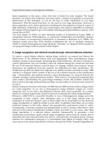
Fig.
11.6
Comparison
of
4
different
MOSFET
models, Levels
1-4.
(After
Khalily
et
al.
[12])
References
56
1
determination of the width and length dependent parameters using
I,,
-

Vgs
data on narrow and short devices. Finally, the velocity saturation and
channel length modulation parameters were extracted using the short
channel length device.
The complete set
of
parameters extracted from
3
different size devices are
then used to simulate other geometries. Figure
11.6
shows the rms error
between the simulated and measured data on different channel length and
width devices. Remember that not all devices were used to extract the
parameters. The Level
2
and Level
3
models show reasonable accuracy in
all geometries except when the channel length is
1.4
pm (effective width of
0.3pm). Note that the Level
1
model does not perform even for large
devices. The
BSIM
model provides excellent accuracy near the geometries
used to extract the parameter values. However, larger deviation between
the measured and simulated results were encountered

for different geome-
tries. This shows that some parameters do not scale well using the
1/L
and
1/W
geometry dependence assumed in Level
4
model.
References
[l]
A. Vladimirescu and
S.
Liu, ‘The simulation of MOS integrated circuits using SPICET,
Memorandum
No.
UCB/ERL
M80/7,
Electronics Research Laboratory, University
of California, Berkeley, October
1980.
[2]
B.
J.
Sheu, D.
L.
Scharfetter, and
H.
C. Poon, ‘Compact short-channel IGFET model
(CSIM),’ Memorandum No. UCB/ERL M84/20, Electronics Research Laboratory,
University of California, Berkeley, March

1984.
[3]
B.
J.
Sheu,
D.
L. Scharfetter, P.
K. KO,
and M. C. Jeng, ‘BSIM: Berkeley short-channel
IGFET model for MOS transistors’, IEEE J. Solid-state Circuits, SC-22, pp.
558-565
(1
987).
[4]
D.
K.
Schroder,
Semiconductor Material and Device Characterization,
John Wiley
&
Sons
Inc., New York, 1990.
[5]
G.
W.
Neudeck,
The
PN
Junction Diode,
Vol.

11,
2nd Ed., Modular Series
on
Solid-
State Devices, Addison-Wesley Publishing Co., Reading MA,
1987.
[6]
D.
J.
Roulston,
Bipolar Semiconductor Devices,
McGraw-Hill Publishing Company,
New York,
1990.
[7]
H. J. Kuno, ‘Analysis and characterization of
pn
junction diode switching’, IEEE
Trans. Electron Dev., ED-11, pp.
8-14 (1964).
181
AH. C. Fung, ‘A subthreshold conduction model for BSIM’, Memorandum
No.
UCB/ERL M85/22, Electronics Research Laboratory, University of California,
Berkeley, October
1985.
[9]
D. Ward, ‘Charge-based modeling of capacitances in MOS transistors’, Stanford
University Tech. Rep.
G201-11, 1982.

[lo]
B.
S.
Messenger, ‘A
fully
automated
MOS
device characterization system
for
process-
oriented integrated circuit design’, Memorandum No. UCB/ERL M84/18, Electronic
Research Laboratory, University of California, Berkeley, January
1984.
[11]
M.
G.
Hsu
and B.
J.
Sheu, ‘Inverse-geometry dependence of MOS transistor electrical
parameters,’ IEEE Trans Computer-Aided Design, CAD-6, pp. 582-585
(1987).