A Practical Introduction to Structure, Mechanism, and Data Analysis - Part 4 ppsx
Bạn đang xem bản rút gọn của tài liệu. Xem và tải ngay bản đầy đủ của tài liệu tại đây (409.46 KB, 41 trang )
4.7.3 Size Exclusion Chromatography
Size exclusion chromatography is commonly used to separate proteins from
small molecular weight species in what are referred to as protein desalting
methods (see Copeland, 1994, and Chapter 7). Because of the nature of the
stationary phase in these columns, macromolecules are excluded and pass
through the columns in the void volume. Small molecular weight species, such
as salts or free ligand molecules, are retained longer within the stationary
phase. Traditional size exclusion chromatography requires tens of minutes to
hours to perform, and is thus usually inappropriate for ligand binding
measurements. Two variations of size exclusion chromatography are, however,
quite useful for this purpose.
In the first variation that is useful for ligand binding measurements, spin
columns are employed for size exclusion chromatography (Penefsky, 1977;
Zeeberg and Caplow, 1979; Anderson and Vaughan, 1982; Copeland, 1994).
Here a small bed volume size exclusion column is constructed within a column
tube that fits conveniently into a microcentrifuge tube. Separation of excluded
and retained materials is accomplished by centrifugal force, rather than by
gravity or peristaltic pressure, as in conventional chromatography. After the
column has been equilibrated with buffer, a sample of the equilibrated
receptor—ligand mixture is applied to the column. A separate sample of the
mixture is retained for measurement of total ligand concentration. The column
is then centrifuged according to the manufacturer’s instructions, and the
excluded material is collected at the bottom of the microcentrifuge tube. This
excluded material contains the protein-bound ligand population. By quantify-
ing the ligand concentration in the sample before centrifugation and in the
excluded material, one can determine the total and bound ligand concentra-
tions, respectively. Again, by subtraction, one can also calculate the free ligand
concentration and thus determine the dissociation constant. Prepacked spin
columns, suitable for these studies are now commercially available from a
number of manufacturers (e.g., BioRad, AmiKa Corporation).
The second variation of size exclusion chromatography that is applicable to
ligand binding measurements is known as Hummel—Dreyer chromatography
(HDC: Hummel and Dreyer, 1962; Ackers, 1973; Cann and Hinman, 1976).In
HDC the size exclusion column is first equilibrated with ligand at a known
concentration. A receptor solution is equilibrated with ligand at the same
concentration as the column, and this solution is applied to the column. The
column is then run with isocratic elution using buffer containing the same
concentration of ligand. Elution is typically followed by measuring some
unique signal from the ligand (e.g., radioactivity, fluorescence, a unique
absorption signal). If there is no binding of ligand to the protein, the signal
measured during elution should be constant and related to the concentration of
ligand with which the column was equilibrated. If, however, binding occurs, the
total concentration of ligand that elutes with the protein will be the sum of the
102 PROTEIN LIGAND BINDING EQUILIBRIA
Figure 4.16 Binding of 2-cytidylic acid to the enzyme ribonuclease as measured by Hum-
mel—Dreyer chromatography. The positive peak of ligand absorbance is coincident with the
elution of the enzyme. The trough at latter time results from free ligand depletion from the
column due to the binding events. [Data redrawn from Hummel and Dreyer (1962).]
bound and free ligand concentrations. Hence, during protein elution the net
signal from ligand elution will increase by an amount proportional to the
bound ligand concentration. The ligand that is bound to the protein is
recruited from the general pool of free ligand within the column stationary and
mobile phases. Hence, some ligand depletion will occur subsequent to protein
elution. This results in a period of diminished ligand concentration during the
chromatographic run. The degree of ligand diminution in this phase of the
chromatograph is also proportional to the concentration of bound ligand.
Figure 4.16 illustrates the results of a typical chromatographic run for an
HDC experiment. From generation of a standard curve (i.e., signal as a
function of known concentration of ligand), the signal units can be converted
into molar concentrations of ligand. From the baseline measurement, one
determines the free ligand concentration (which also corresponds to the
concentration of ligand used to equilibrate the column), while the bound ligand
concentration is determined from the signal displacements that are observed
during and after protein elution (Figure 4.16). Because the column is equilib-
rated with ligand throughout the chromatographic run, displacement from
equilibrium is not a significant concern in HDC. This method is considered by
many to be one of the most accurate measures of protein—ligand equilibria.
Oravcova et al. (1996) have recently reviewed HDC and other methods
applicable to protein—ligand binding measurements; their paper provides a
good starting point for acquiring a more in-depth understanding of many of
these methods.
EXPERIMENTAL METHODS FOR MEASURING LIGAND BINDING 103
4.7.4 Spectroscopic Methods
The receptor—ligand complex often exhibits a spectroscopic signal that is
distinct from the free receptor or ligand. When this is the case, the spectro-
scopic signal can be utilized to follow the formation of the receptor—ligand
complex, and thus determine the dissociation constant for the complex.
Examples exist in the literature of distinct changes in absorbance, fluorescence,
circular dichroism, and vibrational spectra (i.e., Raman and infrared spectra)
that result from receptor—ligand complex formation. The bases for these
spectroscopic methods are not detailed here because they have been presented
numerous times (see Chapter 7 of this text; Campbell and Dwek, 1984;
Copeland, 1994). Instead we shall present an overview of the use of such
methods for following receptor—ligand complex formation.
Because of its sensitivity, fluorescence spectroscopy is often used to follow
receptor—ligand interactions, and we shall use this method as an example.
Often a ligand will have a fluorescence signal that is significantly enhanced or
quenched (i.e., diminished) upon interaction with the receptor. For example,
warfarin and dansylsulfonamide are two fluorescent molecules that are known
to bind to serum albumin. In both cases the fluorescence signal of the ligand
is significantly increased upon complex formation, and knowledge of this
behavior has been used to measure the interactions of these ligands with
albumin (Epps et al., 1995). In contrast, ligand fluorescence can also often be
quenched by interaction with the receptor. For example, my group synthesized
a tripeptide, Lys-Cys-Lys, which we expected to bind to the kringle domains
of plasminogen (Balciunas et al., 1993). We then chemically modified the
peptide with a stilbene—maleimide derivative to impart a fluorescence signal
(via covalent modification of the cysteine thiol). The stilbene-labeled peptide
was highly fluorescent in solution, but it displayed significant fluorescence
quenching upon complex formation with plasminogen and other kringle-
containing proteins (Figure 4.17)
Even when the fluorescence intensity of the ligand is not significantly
perturbed by binding to the receptor, it is often possible to follow receptor—
ligand interaction by a technique known as fluorescence polarization. Fluor-
escence occurs when light of an appropriate wavelength excites a molecule
from its ground electronic state to an excited electronic state (Copeland, 1994).
One means of relaxation back to the ground state is by emission of light energy
(fluorescence). The transitions between the ground and excited states are
accompanied by a redistribution of electron density within the molecule, and
this usually occurs mainly along one axis of the molecule (Figure 4.18). The
axis along which electron density is perturbed between the ground and excited
state is referred to as the transition dipole moment of the molecule.
If the excitation light beam is plane-polarized (by passage through a
polarizing filter), the efficiency of fluorescence will depend on the alignment of
the plane of light polarization with the transition dipole moment. Suppose that
for a particular molecule the transition dipole moment is aligned with the plane
104 PROTEIN LIGAND BINDING EQUILIBRIA
Figure 4.17 Fluorescence spectra of a fluorescently labeled peptide (Lys-Cys-Lys) free in
solution (peptide—dye complex) and bound to the protein plasminogen. Note the significant
quenching of the probe fluorescence upon peptide—plasminogen binding. [Data from Balciunas
et al. (1993).]
of light polarization at the moment of excitation (i.e., light absorption by the
molecule). In this case the light emitted from the molecule will also be plane-
polarized and will thus pass efficiently through a properly oriented polarization
filter placed between the sample and the detector. In this sequence (Figure
4.18A), the molecule has not rotated in space during its excited state lifetime,
and so the plane of polarization remains the same. This is not always the case,
however. If the molecule rotates during the excited state, less fluorescent light
will pass through the oriented polarization filter between the sample and the
detector: the faster the rotation, the less light passes (Figure 4.18B). Hence, as
the rotational rate of the molecule is slowed down, the efficiency of fluorescence
polarization increases. Small molecular weight ligands rotate in solution much
faster than macromolecules, such as proteins. Hence, when a fluorescent ligand
binds to a much larger protein, its rate of rotation in solution is greatly
diminished, and a corresponding increase in fluorescence polarization is
observed. This is the basis for measuring protein—ligand interactions by
fluorescence polarization. A more detailed description of this method can be
found in the texts by Campbell and Dwek (1984) and Lackowicz (1983). The
PanVera Corporation (Madison, WI) also distributes an excellent primer and
applications guide on the use of fluorescence polarization measurements for
studying protein—ligand interactions.
EXPERIMENTAL METHODS FOR MEASURING LIGAND BINDING 105
Figure 4.18 Schematic illustration of fluorescence polarization, in which a plane polarizing
filter between the light source and the sample selects for a single plane of light polarization.
The plane of excitation light polarization is aligned with the transition dipole moment (illustrated
by the gray double-headed arrow) of the fluorophore there, the amino acid tyrosine. The emitted
light is also plane-polarized and can thus pass through a polarizing filter, between the sample
and detector, only if the plane of the emitted light polarization is aligned with the filter. (A) The
molecule does not rotate during the excited state lifetime. Hence, the plane of polarization of
the emitted light remains aligned with that of the excitation beam. (B) The molecule has rotated
during the excited state lifetime so that the polarization planes of the excitation light and the
emitted light are no longer aligned. In this latter case, the emitted light is said to have undergone
depolarization.
Proteins often contain the fluorescent amino acids tryptophan and tyrosine
(Campbell and Dwek, 1984; Copeland, 1994), and in some cases the intrinsic
fluoresence of these groups is perturbed by ligand binding to the protein. There
are a number of examples in the literature of proteins containing a tryptophan
residue at or near the binding site for some ligand. Binding of the ligand in
these cases often results in a change in fluorescence intensity and/or wavelength
maximum for the affected tryptophan. Likewise, tyrosine-containing proteins
often display changes in tyrosine fluorescence intensity upon complex forma-
106 PROTEIN LIGAND BINDING EQUILIBRIA
tion with ligand. A number of DNA binding proteins, for example, display
dramatic quenching of tyrosine fluorescence when DNA is bound to them.
Any spectroscopic signal that displays distinct values for the bound and free
versions of the spectroscopically active component (either ligand or receptor),
can be used as a measure of protein—ligand complex formation. Suppose that
some signal has one distinct value for the free species
and another value
for the bound species
. If the spectroscopically active species is the
receptor, then the concentration of receptor can be fixed, and the signal at any
point within a ligand titration will be given by:
: [RL]
; [R]
(
)(4.40)
Since [R]
is equivalent to [R] 9 [RL], we can rearrange this equation to:
: [RL](
9
) ; [R](
)(4.41)
Equation 4.41 can be rearranged further to give the fraction of bound receptor
at any point in the ligand titration as follows:
[RL]
[R]
:
9
9
(4.42)
Similarly, if the spectroscopically active species is the ligand, a fixed concentra-
tion of ligand can be titrated with receptor, and the fraction of bound ligand
can be determined as follows:
[RL]
[L]
:
9
9
(4.43)
The dissociation constant for the receptor—ligand complex can then be deter-
mined from isothermal analysis of the spectroscopic titration data as described
above.
4.8 SUMMARY
In this chapter we have described methods for the quantitative evaluation of
protein—ligand binding interactions at equilibrium. The Langmuir binding
isotherm equation was introduced as a general description of protein—ligand
equilibria. From fitting of experimental data to this equation, estimates of the
equilibrium dissociation constant K
and the concentration of ligand binding
sites n, can be obtained. We shall encounter the Langmuir isotherm equation
in different forms throughout the remainder of this text in our discussions of
enzyme interactions with ligands such as substrates inhibitors and activators.
SUMMARY 107
The basic concepts described here provide a framework for understanding the
kinetic evaluation of enzyme activity and inhibition, as discussed in these
subsequent chapters.
REFERENCES AND FURTHER READING
Ackers, G. K. (1973) Methods Enzymol. 27, 441.
Anderson, K. B., and Vaughan, M. H. (1982) J. Chromatogr. 240,1.
Balciunas, A., Fless, G., Scanu, A., and Copeland, R. A. (1993) J. Protein Chem. 12, 39.
Bell, J. E., and Bell, E. T. (1988) Proteins and Enzymes, Prentice-Hall, Englewood Cliffs,
NJ.
Campbell, I. D., and Dwek, R. A. (1984) Biological Spectroscopy, Benjamin/Cummings,
Menlo Park, CA.
Cann, J. R., and Hinman, N. D. (1976) Biochemistry, 15, 4614.
Copeland, R. A. (1994) Methods for Protein Analysis: A Practical Guide to L aboratory
Protocols, Chapman & Hall, New York.
Englund, P. T., Huberman, J. A., Jovin, T. M., and Kornberg, A. (1969) J. Biol. Chem.
244, 3038.
Epps, D. E., Raub, T. J., and Kezdy, F. J. (1995) Anal. Biochem. 227, 342.
Feldman, H. A. (1972) Anal. Biochem. 48, 317.
Freundlich, R. and Taylor, D. B. (1981) Anal. Biochem. 114, 103.
Halfman, C. J., and Nishida, T. (1972) Biochemistry, 18, 3493.
Hulme, E. C. (1992) Receptor—L igand Interactions: A Practical Approach, Oxford
University Press, New York.
Hummel, J. R., and Dreyer, W. J. (1962) Biochim. Biophys. Acta, 63, 530.
Klotz, I. M. (1997) L igand—Receptor Energetics: A Guide for the Perplexed, Wiley, New
York.
Lackowicz, J. R. (1983) Principle of Fluorescence Spectroscopy, Plenum Press, New
York.
Oravcova, J., Bo¨ hs, B., and Lindner, W. (1996) J. Chromatogr. B 677,1.
Paulus, H. (1969) Anal. Biochem. 32, 91.
Penefsky, H. S. (1977) J. Biol. Chem. 252, 2891.
Perutz, M. (1990) Mechanisms of Cooperativity and Allosteric Regulation in Proteins,
Cambridge University Press, New York.
Segel, I. H. (1976) Biochemical Calculations, 2nd ed., Wiley, New York.
Wolff, B. (1930) In Enzymes, J. B. S. Haldane, Ed., Longmans, Green & Co., London.
Wolff, B. (1932) In Allgemeine Chemie der Enzyme, J. B. S. Haldane and K. G. Stern,
Eds., Steinkopf, Dresden, pp. 119ff.
Zeeberg, B., and Caplow, M. (1979) Biochemistry, 18, 3880.
108 PROTEIN LIGAND BINDING EQUILIBRIA
5
KINETICS OF
SINGLE-SUBSTRATE
ENZYME REACTIONS
Enzyme-catalyzed reactions can be studied in a variety of ways to explore
different aspects of catalysis. Enzyme—substrate and enzyme—inhibitor com-
plexes can be rapidly frozen and studied by spectroscopic means. Many
enzymes have been crystallized and their structures determined by x-ray
diffraction methods. More recently, enzyme structures have been determined
by multidimensional NMR methods. Kinetic analysis of enzyme-catalyzed
reactions, however, is the most commonly used means of elucidating enzyme
mechanism and, especially when coupled with protein engineering, identifying
catalytically relevant structural components. In this chapter we shall explore
the use of steady state and transient enzyme kinetics as a means of defining the
catalytic efficiency and substrate affinity of simple enzymes. As we shall see, the
term steady state refers to experimental conditions in which the enzyme—
substrate complex can build up to an appreciable ‘‘steady state’’ level. These
conditions are easily obtained in the laboratory, and they allow for convenient
interpretation of the time courses of enzyme reactions. All the data analysis
described in this chapter rests on the ability of the scientist to conveniently
measure the initial velocity of the enzyme-catalyzed reaction under a variety of
conditions. For our discussion, we shall assume that some convenient method
for determining the initial velocity of the reaction exists. In Chapter 7 we shall
address specifically how initial velocities are measured and describe a variety of
experimental methods for performing such measurements.
5.1 THE TIME COURSE OF ENZYMATIC REACTIONS
Upon mixing an enzyme with its substrate in solution and then (by some
convenient means) measuring the amount of substrate remaining and/or the
109
Enzymes: A Practical Introduction to Structure, Mechanism, and Data Analysis.
Robert A. Copeland
Copyright
2000 by Wiley-VCH, Inc.
ISBNs: 0-471-35929-7 (Hardback); 0-471-22063-9 (Electronic)
Figure 5.1 Reaction progress curves for the loss of substrate [S] and production of product
[P] during an enzyme-catalyzed reaction.
amount of product produced over time, one will observe progress curves similar
to those shown in Figure 5.1. Note that the substrate depletion curve is the
mirror image of the product appearance curve. At early times substrate loss
and product appearance change rapidly with time but as time increases these
rates diminish, reaching zero when all the substrate has been converted to
product by the enzyme. Such time courses are well modeled by first-order
kinetics, as discussed in Chapter 2:
[S] : [S
]e\IR (5.1)
where [S] is the substrate concentration remaining at time t,[S
] is the starting
substrate concentration, and k is the pseudo-first-order rate constant for the
reaction. The velocity v of such a reaction is thus given by:
v :9
d[S]
dt
:
d[P]
dt
: k[S
]e\IR (5.2)
Let us look more carefully at the product appearance profile for an enzyme-
catalyzed reaction (Figure 5.2). If we restrict our attention to the very early
portion of this plot (shaded area), we see that the increase in product formation
(and substrate depletion as well) tracks approximately linear with time. For
this limited time period, the initial velocity v
can be approximated as the slope
(change in y over change in x) of the linear plot of [S] or [P] as a function of
time:
v
:9
[S]
t
:
[P]
t
(5.3)
110 KINETICS OF SINGLE-SUBSTRATE ENZYME REACTIONS
Figure 5.2 Reaction progress curve for the production of product during an enzyme-catalyzed
reaction. Inset highlights the early time points at which the initial velocity can be determined
from the slope of the linear plot of [P] versus time.
Experimentally one finds that the time course of product appearance and
substrate depletion is well modeled by a linear function up to the time when
about 10% of the initial substrate concentration has been converted to product
(Chapter 2). We shall see in Chapter 7 that by varying solution conditions, we
can alter the length of time over which an enzyme-catalyzed reaction will
display linear kinetics. For the rest of this chapter we shall assume that the
reaction velocity is measured during this early phase of the reaction, which
means that from here v : v
, the initial velocity.
5.2 EFFECTS OF SUBSTRATE CONCENTRATION ON VELOCITY
From Equation 5.2, one would expect the velocity of a pseudo-first-order
reaction to depend linearly on the initial substrate concentration. When early
studies were performed on enzyme-catalyzed reactions, however, scientists
found instead that the reactions followed the substrate dependence illustrated
in Figure 5.3. Figure 5.3A illustrates the time course of the enzyme-catalyzed
reaction observed at different starting concentrations of substrate; the velocities
for each experiment are measured as the slopes of the plots of [P] versus time.
Figure 5.3B replots these data as the initial velocity v as a function of [S], the
starting concentration of substrate. Rather than observing the linear relation-
ship expected for first-order kinetics, we find the velocity apparently saturable
at high substrate concentrations. This behavior puzzled early enzymologists.
EFFECTS OF SUBSTRATE CONCENTRATION ON VELOCITY 111
Figure 5.3 (A) Progress curves for a set of enzyme-catalyzed reactions with different starting
concentrations of substrate [S]. (B) Plot of the reaction velocities, measured as the slopes of
the lines from (A), as a function of [S].
Three distinct regions of this curve can be identified: at low substrate
concentrations the velocity appears to display first-order behavior, tracking
linearly with substrate concentration; at very high concentrations of substrate,
the velocity switches to zero-order behavior, displaying no dependence on
substrate concentration; and in the intermediate region, the velocity displays a
curvilinear dependence on substrate concentration. How can one rationalize
these experimental observations?
A qualitative explanation for the substrate dependence of enzyme-catalyzed
reaction velocities was provided by Brown (1902). At the same time that the
112 KINETICS OF SINGLE-SUBSTRATE ENZYME REACTIONS
kinetic characteristics of enzyme reactions were being explored, evidence for
complex formation between enzymes and their substrates was also accumulat-
ing. Brown thus argued that enzyme-catalyzed reactions could best be de-
scribed by the following reaction scheme:
E ; S
I
&
I\
ES
I
-
E ; P
This scheme predicts that the reaction velocity will be proportional to the
concentration of the ES complex as: v : k
[ES]. Suppose that we held the total
enzyme concentration constant at some low level and varied the concentration
of S. At low concentrations of S the concentration of ES would be directly
proportional to [S]; hence the velocity would depend on [S] in an apparent
first-order fashion. At very high concentrations of S, however, practically all
the enzyme would be present in the form of the ES complex. Under such
conditions the velocity depends of the rate of the chemical transformations that
convert ES to EP and the subsequent release of product to re-form free
enzyme. Adding more substrate under these conditions would not effect a
change in reaction velocity; hence the slope of the plot of velocity versus [S]
would approach zero (as seen in Figure 5.3B). The complete [S] dependence of
the reaction velocity (Figure 5.3B) predicted by the model of Brown resembles
the results seen from the Langmuir isotherm Equation (Chapter 4) for
equilibrium binding of ligands to receptors. This is not surprising, since in the
model of Brown, catalysis is critically dependent on initial formation of a
binary ES complex through equilibrium binding.
5.3 THE RAPID EQUILIBRIUM MODEL OF ENZYME KINETICS
Although the model of Brown provided a useful qualitative picture of enzyme
reactions, to be fully utilized by experimental scientists, it needed to be put into
a rigorous mathematical framework. This was accomplished first by Henri
(1903) and subsequently by Michaelis and Menten (1913). Ironically, Michaelis
and Menten are more widely recognized for this contribution, although they
themselves acknowledged the prior work of Henri. The basic rate equation
derived in this section is commonly referred to as the Michaelis—Menten
equation. Several writers have recently taken to referring to the equation as the
Henri—Michaelis—Menten equation, in an attempt to correct this neglect of
Henri’s contributions. The reader should be aware, however, that the majority
of the scientific literature continues to use the traditional terminology.
The Henri—Michaelis—Menten approach assumes that a rapid equilibrium is
established between the reactants (E ; S) and the ES complex, followed by
slower conversion of the ES complex back to free enzyme and product(s); that
is, this model assumes that k
k
\
in the scheme presented in Section 5.2. In
THE RAPID EQUILIBRIUM MODEL OF ENZYME KINETICS 113
this model, the free enzyme E
first combines with the substrate S to form the
binary ES complex. Since substrate is present in large excess over enzyme, we
can use the assumption that the free substrate concentration [S]
is well
approximated by the total substrate concentration added to the reaction [S].
Hence, the equilibrium dissociation constant for this complex is given by:
K
1
:
[E]
[S]
[ES]
(5.4)
Similar to the treatment of receptor—ligand binding in Chapter 4, here the free
enzyme concentration is given by the difference between the total enzyme
concentration [E] and the concentration of the binary complex [ES]:
[E]
: [E] 9 [ES] (5.5)
and therefore,
K
1
:
([E] 9 [ES])[S]
[ES]
(5.6)
This can be rearranged to give an expression for [ES]:
[ES] :
[E][S]
K
1
; [S]
(5.7)
Next, the ES complex is transformed by various chemical steps to yield the
product of the reaction and to recover the free enzyme. In the simplest case, a
single chemical step, defined by the first-order rate constant k
, results in
product formation. More likely, however, there will be a series of rapid
chemical events following ES complex formation. For simplicity, the overall
rate for these collective chemical steps can be described by a single first-order
rate constant k
. Hence:
E ; S
&
)
1
ES
I
99; E ; P
and the rate of product formation is thus given by the first-order equation:
v : k
[ES] (5.8)
Combining Equations 5.7 and 5.8, we obtain:
v :
k
[E][S]
K
1
; [S]
(5.9)
114 KINETICS OF SINGLE-SUBSTRATE ENZYME REACTIONS
Equation 5.9 is similar to the equation for a Langmuir isotherm, as derived in
Chapter 4 (Equation 4.21). This, then, describes the reaction velocity as a
hyperbolic function of [S], with a maximum value of k
[E] at infinite [S]. We
refer to this value as the maximum reaction velocity, or V
.
V
: k
[E] (5.10)
Combining this definition with Equation 5.9, we obtain:
v :
V
[S]
K
1
; [S]
:
V
1 ;
K
1
[S]
(5.11)
Equation 5.11 is the final equation derived independently by Henri and
Michaelis and Menten to describe enzyme kinetic data. Note the striking
similarity between this equation and the forms of the Langmuir isotherm
equation presented in Chapter 4 (Equations 4.21 and 4.22). Thus, much of
enzyme kinetics can be explained in terms of a simple equilibrium model
involving rapid equilibrium between free enzyme and substrate to form the
binary ES complex, followed by chemical transformation steps to produce and
release product.
5.4 THE STEADY STATE MODEL OF ENZYME KINETICS
The original derivations by Henri and by Michaelis and Menten depended on
a rapid equilibrium approach to enzyme reactions. This approach is quite
useful in rapid kinetic measurements, such as single-turnover reactions, as
described later in this chapter. The majority of experimental measurements of
enzyme reactions, however, occur when the ES complex is present at a
constant, steady state concentration (as defined below). Briggs and Haldane
(1925) recognized that the equilibrium-binding approach of Henri and
Michaelis and Menten could be described more generally by a steady state
approach that did not require k
k
\
. The following discussion is based on
this description by Briggs and Haldane. As we shall see, the final equation that
results from this treatment is very similar to Equation 5.11, and despite the
differences between the rapid equilibrium and steady state approaches, the final
steady state equation is commonly referred to as the Henri—Michaelis—Menten
equation.
Steady state refers to a time period of the enzymatic reaction during which
the rate of formation of the ES complex is exactly matched by its rate of decay
to free enzyme and products. This kinetic phase can be attained when the
concentration of substrate molecules is in great excess of the free enzyme
concentration. To achieve a steady state, certain condition must be met, and
THE STEADY STATE MODEL OF ENZYME KINETICS 115
these conditions allow us to make some reasonable assumption, which greatly
simplify the mathematical treatment of the kinetics. These assumptions are as
follows:
1. During the initial phase of the reaction progress curve (i.e., conditions
under which we are measuring the linear initial velocity), there is no
appreciable buildup of any intermediates other than the ES complex.
Hence, all the enzyme molecules can be accounted for by either the free
enzyme or by the enzyme—substrate complex. The total enzyme concen-
tration [E] is therefore given by:
[E] : [E]
; [ES] (5.12)
2. As in the rapid equilibrium treatment, we assume that the enzyme is
acting catalytically, so that it is present in very low concentration relative
to substrate, that is, [S] [E]. Hence, formation of the ES complex does
not significantly diminish the concentration of free substrate. We can
therefore make the approximation: [S]
: [S], where [S]
is the free
substrate concentration and [S] is the total substrate concentration).
3. During the initial phase of the progress curve, very little product is
formed relative to the total concentration of substrate. Hence, during this
early phase [P] : 0 and therefore depletion of [S] is minimal. At the
initiation of the reaction there will be a rapid burst of formation of the
ES complex followed by a kinetic phase in which the rate of formation
of new ES complex is balanced by the rate of its decomposition back to
free enzyme and product. In other words, during this phase the concen-
tration of ES is constant. We refer to this kinetic phase as the steady state,
which is defined by:
d[ES]
dt
: 0 (5.13)
Figure 5.4 illustrates the development and duration of the steady state for
the enzyme cytochrome c oxidase interacting with its substrates cytochrome c
and molecular oxygen. As soon as the substrates and enzyme are mixed, we see
a rapid pre—steady state buildup of ES complex, followed by a long time
window in which the concentration of ES does not change (the steady state
phase), and finally a post—steady state phase characterized by significant
depletion of the starting substrate concentration.
With these assumptions made, we can now work out an expression for the
enzyme velocity under steady state conditions. As stated previously, for the
simplest of reaction schemes, the pseudo-first-order progress curve for an
enzymatic reaction can be described by:
v : k
[ES] (5.14)
116 KINETICS OF SINGLE-SUBSTRATE ENZYME REACTIONS
Figure 5.4 Development of the steady state for the reaction of cytochrome c oxidase with its
substrates, cytochrome c and molecular oxygen. The absorbance at 444 nm reflects the ligation
state of the active site heme cofactor of the enzyme. Prior to substrate addition (time : 0) the
heme group is in the Fe
3;
oxidation state and is ligated by a histidine group from the enzyme.
Upon substrate addition, the active site heme iron is reduced to the Fe
2
> state and rapidly
reaches a steady state phase of substrate utilization in which the iron is ligated by some oxygen
species. The steady state phase ends when a significant portion of the molecular oxygen in
solution has been used up. At this point the heme iron remains reduced (Fe
2
>) but is no longer
bound to a ligand at its sixth coordination site; this heme species has a much larger extinction
coefficient at 444 nm; hence the rapid increase in absorbance at this wavelength following the
steady state phase. [Data adapted and redrawn from Copeland (1991).]
Now, [ES] is dependent on the rate of formation of the complex (governed by
k
) and the rate of loss of the complex (governed by k
\
and k
). The rate
equations for these two processes are thus given by:
d[ES]
dt
: k
[E]
[S]
and
9d[ES]
dt
: (k
\
; k
)[ES] (5.15)
Under steady state conditions these two rates must be equal, hence:
k
[E]
[S]
: (k
\
; k
)[ES] (5.16)
This can be rearranged to obtain an expression for [ES]:
[ES] :
[E]
[S]
k
\
; k
k
(5.17)
THE STEADY STATE MODEL OF ENZYME KINETICS 117
At this point let us define the term K
as an abbreviation for the kinetic
constants in the denominatior of the right-hand side of Equation 5.17:
K
:
k
\
; k
k
(5.18)
For now we will consider K
to be merely an abbreviation to make our
subsequent mathematical expressions less cumbersome. Later, however, we
shall see that K
has a more significant meaning. Substituting Equation 5.18
into Equation 5.17 we obtain:
[ES] :
[E]
[S]
K
(5.19)
Now, since substrate depletion is insignificant during the steady state phase, we
can replace the term [S]
by the total substrate concentration [S] (which is
much more easily measured in real experimental situations). We can also use
the equality of Equation 5.12 to replace [E]
by ([E] 9 [ES]). With these
substitutions, Equation 5.19 can be recast as follows:
[ES] : [E]
[S]
[S] ; K
(5.20)
If we now combine this expression for [ES] with the velocity expression of
Equation 5.14, we obtain:
v : k
[E]
[S]
[S] ; K
(5.21)
Or, we can generalize Equation 5.21 for more complex reaction schemes by
substituting k
for k
:
v : k
[E]
[S]
[S] ; K
(5.22)
As described earlier, as the concentration of substrate goes towards infinity, the
velocity reaches a maximum value that we have defined as V
. Under these
conditions, the K
term is a very small contribution to Equation 5.22.
Therefore:
lim
1
[S]
[S] ; K
5
[S]
[S]
: 1 (5.23)
and thus we again arrive at Equation 5.10: V
: k
[E]. Combining this with
118 KINETICS OF SINGLE-SUBSTRATE ENZYME REACTIONS
Equation 5.23 we finally arrive at an expression very similar to that first
described by Henri and Michaelis and Menten (i.e., similar to Equation 5.11):
v :
V
[S]
K
; [S]
:
V
1 ;
K
[S]
(5.24)
This is the central expression for steady state enzyme kinetics. While it differs
from the equilibrium expression derived by Henri and by Michaelis and
Menten, it is nevertheless universally referred to as the Michaelis—Menten or
Henri—Michaelis—Menten equation.
In our definition of K
(Equation 5.18), we combined first-order rate
constants (k
\
and k
, which have units of reciprocal time) with a second-order
rate constant (k
, which has units of reciprocal molarity, reciprocal time) in
such a way that the resulting K
has units of molarity, as does [S]. If we set
up our experimental system so that the concentration of substrate exactly
matches K
, Equation 5.24 will reduce to:
v :
V
[S]
[S] ; [S]
:
V
2
(5.25)
This provides us with a working definition of K
: The K
is the substrate
concentration that provides a reaction velocity that is half of the maximal velocity
obtained under saturating substrate conditions. The K
value is often referred to
in the literature as the Michaelis constant. In comparing Equation 5.24 for
steady state kinetics with Equation 5.11 for the rapid equilibrium treatment,
we see that the equations are identical except for the substitution of K
for K
1
in the steady state treatment. It is therefore easy to confuse these terms and to
treat K
as if it were the thermodynamic dissociation constant for the ES
complex. However, the two constants are not always equal, even in consider-
ations of the simplest of reactions schemes, as here. Recall that K
1
can be
defined by the rato of the reverse and forward reaction rate constants:
K
1
:
k
\
k
(5.26)
This value is not identical to the expression for K
given in Equation 5.18.
Only under the specific conditions that k
k
\
are K
and K
1
equivalent.
For more complex reaction schemes one would replace the k
term in Equation
5.18 by k
. Recall that k
reflects a summation of multiple chemical steps in
catalysis. Hence, depending on the details of the reaction mechanism, and the
values of the individual rate constants, situations can arise in which the value
of K
is less than, greater than, or equal to K
1
. Therefore, K
should generally
be considered as a kinetic, not thermodynamic, constant.
THE STEADY STATE MODEL OF ENZYME KINETICS 119
5.5 THE SIGNIFICANCE OF
k
cat
AND
K
m
We have gone to great lengths in this chapter to define and derive expressions
for the kinetic constants k
and K
. What value do these constants add to
our understanding of the enzyme under study?
5.5.1
K
m
The value of K
varies considerably from one enzyme to another, and for a
particular enzyme with different substrates. We have already defined K
as the
substrate concentration that results in half-maximal velocity for the enzymatic
reaction. An equivalent way of stating this is that the K
represents the
substrate concentration at which half of the enzyme active sites in the sample
are filled (i.e., saturated) by substrate molecules in the steady state. Hence,
while K
is not equivalent to K
1
under most conditions, it can nevertheless be
used as a relative measure of substrate binding affinity. In some instances,
changes in solution conditions (pH, temperature, etc.) can have selective effects
on the value of K
. Also, one sometimes observes effects on the value of K
in
the course of comparing different mutants or isoforms of an enzyme, or
different substrates with a common enzyme. In these cases one can reasonably
relate the changes to effects on the stability (i.e., affinity) of the ES complex. As
we shall see below, however, the ratio k
/K
is generally a better measure of
effects on substrate binding.
5.5.2
k
cat
Considering Equations 5.22—5.24, we see that if one knows the concentration
of enzyme used experimentally, the value of k
can be directly calculated by
dividing the experimentally determined value of V
by [E]. The value of k
is sometimes referred to as the turnover number for the enzyme, since it defines
the number of catalytic turnover events that occur per unit time. The units of
k
are reciprocal time (e.g., min\,s\). Turnover numbers, however, are
typically reported in units of molecules of product produced per unit time per
molecules of enzyme present. As long as the same units are used to express the
amount of product produced and the amount of enzyme present, these units
will cancel and, as expected, the final units will be reciprocal time. It is
important, however, that the units of product and enzyme concentration be
expressed in molar or molarity units. In crude enzyme samples, such as cell
lysates and other nonhomogeneous protein samples, it is often impossible to
know the concentration of enzyme in anything other than units of total protein
mass. The literature is thus filled with enzyme activity values expressed as
number of micrograms of product produced per minute per microgram of
protein in the enzyme sample. While such units may be useful in comparing
one batch of crude enzyme to another (see the discussion of specific activity
120 KINETICS OF SINGLE-SUBSTRATE ENZYME REACTIONS
measurements in Chapter 7), it is difficult to relate these values to kinetic
constants, such as k
.
In the laboratory we can easily determine the turnover number as k
,by
measuring the reaction velocity under conditions of [S] K
so that v
approaches V
. The rate of enzyme turnover under most physiological
conditions in vivo, however, is very different from our laboratory situation.
In vivo, the concentration of substrate is more typically 0.1—1.0K
. When
[S] K
we must change our expression for velocity to:
v :
k
K
[E][S]
(5.27)
(Since [S] K
here, the free enzyme concentration is well approximated by
the total enzyme concentration [E]; thus we used this term in Equation 5.27
in place of [E]
.) Recalling our definition of K
, we note that:
k
K
:
k
k
k
\
; k
(5.28)
Thus, under our laboratory conditions, where [S] K
, formation of the ES
complex is rapid and often is not the rate-limiting step. In vivo, however, where
[S] K
, the overall reaction may be limited by the diffusional rate of
encounter of the free enzyme with substrate, which is defined by k
. The rate
constant for diffusional encounters between molecules like enzymes and sub-
strates is typically in the range of 10—10 M\ s\. Thus we must keep in
mind that the rate-limiting step in catalysis is not always the same in vivo as
in vitro. Nevertheless, measurement of k
(i.e., velocity under saturating
substrate concentration) gives us the most consistent means of comparing rates
for different enzymatic reactions.
The significance of k
is that it defines for us the maximal velocity at which
an enzymatic reaction can proceed at a fixed concentration of enzyme and
infinite availability of substrate. Because k
relates to the chemical steps
subsequent to formation of the ES complex, changes in k
, brought about by
changes in the enzyme (e.g., mutagenesis of specific amino acid residues, or
comparison of different enzymes), in solution conditions (e.g., pH, ionic
strength, temperature, etc.), or in substrate identity (e.g., structural analogues
or isotopically labeled substrates), define perturbations that affect the chemical
steps in enzymatic catalysis. In other words, changes in k
reflect perturba-
tions of the chemical steps subsequent to initial substrate binding. Since k
reflects multiple chemical steps, it does not provide detailed information on the
rates of any of the individual steps subsequent to substrate binding. Instead k
provides a lower limit on the first-order rate constant of the slowest (i.e.,
rate-determining) step following substrate binding that leads eventually to
product release.
THE SIGNIFICANCE OF k
cat
AND K
m
121
5.5.3
k
cat
/
K
m
The catalytic efficiency of an enzyme is best defined by the ratio of the kinetic
constants, k
/K
. This ratio has units of a second-order rate constant and is
generally used to compare the efficiencies of different enzymes to one another.
The values of k
/K
are also used to compare the utilization of different
substrates for a particular enzyme. As we shall see in Chapter 6, in comparisons
of different substrates for an enzyme, the largest differences often are seen in
the values of k
, rather than in K
. This is because substrate specificity often
results from differences in transition state, rather than ground state binding
interactions (see Chapter 6 for more details). Hence, the ratio k
/K
captures
the effects of differing substrate on either kinetic constant and provides a lower
limit for the second-order rate constant of productive substrate binding (i.e.,
substrate binding leading to ES
‡
complex formation and eventual product
formation); this ratio is therefore considered to be the best measure of substrate
specificity.
The ratio k
/K
is also used to compare the efficiency with which an
enzyme catalyzes a particular reaction in the forward and reverse directions.
Enzymatic reactions are in principle reversible, although for many enzymes the
reverse reaction is thermodynamically unfavorable. The presence of an enzyme
in solution does not alter the equilibrium constant K
between the free
substrate and free product concentrations. Hence, the value of K
is fixed for
specific solution conditions, and this constrains the values of k
/K
that can
be achieved in the forward (f) and reverse (r) directions. At equilibrium the
forward and reverse reactions occur with equal frequency so that:
k
K
[E][S] :
k
K
[E][P] (5.29)
hence,
K
:
(k
/K
)
(k
/K
)
(5.30)
Equation 5.30, known as the Haldane relationship, provides a useful measure
of the directionality of an enzymatic reaction under a specific set of solution
conditions.
In either direction, the ratio k
/K
can be related to the free energy
difference between the free reactants (E and S, in the forward direction) and
the transition state complex (ES
‡
). If we normalize the free energy of the
reactant state to zero, the free energy difference is defined by:
G
ES
‡
:9RT ln
k
K
; RT ln
k
T
h
(5.31)
where k
is the Boltzmann constant, T is temperature in degrees Kelvin, and
122 KINETICS OF SINGLE-SUBSTRATE ENZYME REACTIONS
h is Planck’s constant, so that at a fixed temperature the term RT ln(k
T/h) is
a constant. This relationship holds because generally attainment of the transi-
tion state is the most energetically costly component of the multiple steps
contributing to k
. If we compare different substrates for a single enzyme, or
different enzymes or mutants versus a common substrate, we can calculate the
difference in transition state energies (G
#1
‡
) from experimentally measured
values of k
/K
at constant temperature:
G
#1
‡
:9RT ln
(k
/K
)
(k
/K
)
(5.32)
where the superscripts 1 and 2 refer to the different substrates or enzymes being
compared. By this type of analysis, one can quantitate the thermodynamic
contributions of particular structural components to catalysis. For example,
suppose one suspected that an active site tyrosine residue was forming a critical
hydrogen bond with substrate in the transition state of the enzymatic reaction.
Through the tools of molecular biology, one could replace this tyrosine with a
phenylalanine (which would be incapable of forming an H bond) by site-
directed mutagenesis and measure the value of k
/K
for both the wild type
and the Tyr;Phe mutant. Suppose these values turned out to be 88 M\ s\
for the wild-type enzyme and 0.1 M\ s\ for the mutant. The ratio of these
k
/K
would be 880 and, from Equation 5.30, this would correspond to a
difference in transition state free energy of 4 kcal/mol, consistent with a strong
H-bonding interaction of the tyrosine (of course this does not prove that the
exact role of the tyrosine OH group is H-bonding, but the data do prove that
this OH group plays a critical role in catalysis). A good example of the use of
this approach can be found in the paper by Wilkinson et al. (1983).
5.5.4 Diffusion-Controlled Reactions and Kinetic Perfection
For an enzyme in solution, the rate-determining step in catalysis will be either
k
, the rate of ES formation, or one of the multiple steps contributing to k
.
If k
is rate limiting, the catalytic events that occur after substrate binding are
slower that the rate of formation of the ES complex. If, however, k
is rate
limiting, the enzyme turns over essentially instantaneously once the ES
complex has formed. In either case we see that the fastest rate of catalysis for
an enzyme in solution is limited by the rate of diffusion of molecules in the
solution. Some enzymes, such as carbonic anhydrase, display k
/K
values of
10—10 M\ s\, which is at the diffusion limit. Such enzymes are said to have
achieved kinetic perfection, because they convert substrate to product as fast as
the substrate is delivered to the active site of the enzyme!
The diffusion limit would seem to set an upper limit on the value of k
/K
that an enzyme can achieve. This is true for most enzymes in solution.
However, some enzyme systems have overcome this limit by compartmentaliz-
THE SIGNIFICANCE OF k
cat
AND K
m
123
ing themselves and their substrates within close proximity in subcellular locals
where three-dimensional diffusion no longer comes into play. This can be
accomplished by assembling enzymes and substrates into organized systems
such as multienzyme complexes or cellular membranes. Two examples are
presented.
We first consider the respiratory electron transfer system of the inner
mitochondrial membrane. Here enzymes in a cascade are localized in close
proximity to one another within the membrane bilayer. The product of one
enzyme is the substrate for the next in the cascade. Because of the proximity
of the enzymes in the membrane, the product leaves the active site of one
enzyme and is presented to the active site of the next enzyme without the need
for diffusion through solution.
The second example comes from the de novo synthetic pathway for
pyrimidines. The first three steps in the synthesis of uridine monophosphate are
performed by a supercomplex of three enzymes that are noncovalently asso-
ciated as a multiprotein complex. This supercomplex, referred to as CAD,
comprises the enzymes carbamyl phosphate synthase, aspartate transcar-
bamylase, and dihydroorotase. Because the active sites of the three enzymes are
compartmentalized inside the supercomplex, the product of the first enzyme is
immediately in proximity to the active site of the second enzyme, and so on.
In this way, the supercomplex can overcome the diffusion barrier to rapid
catalysis.
5.6 EXPERIMENTAL MEASUREMENT OF
k
cat
AND
K
m
5.6.1 Graphical Determinations from Untransformed Data
The kinetic constants V
and K
are determined graphically with initial
velocity measurements obtained at varying substrate concentrations. The
graphical methods are best illustrated by working through examples with some
numerical data. The quality of the estimates of V
and K
depend on
covering a substrate concentration range that spans a significant portion of the
binding isotherm. Experimentally, a convenient method for choosing substrate
concentrations is to first make a stock solution of substrate at the highest
concentration that is experimentally reasonable. Then, twofold serial dilutions
can be made from this stock to produce a range of lower substrate concentra-
tions. For example, let us say that the highest concentration of substrate to be
used in an enzymatic reaction is 250 M. We could make a 2.5 mM stock
solution of the substrate that would be diluted 10-fold into the final assay
reaction mixture (i.e., to give a final concentration of 250 M). We could then
take a portion of this stock solution and dilute it with an equal volume of
buffer to yield a 1.25 mM solution, which upon dilution into the assay reaction
mixture would give a final substrate concentration of 125 M. A portion of this
solution could also be diluted in half with buffer, and so on, to yield a series
124 KINETICS OF SINGLE-SUBSTRATE ENZYME REACTIONS
Table 5.1 Initial velocity (with random error added) as a function of substrate
concentration for a model enzymatic reaction
[S](M)? v(M product formed s\) 1/v(M\·s) 1/[S](M\)
0.98 10 0.100 1.024
1.95 12 0.083 0.512
3.91 28 0.036 0.256
7.81 40 0.025 0.128
15.63 55 0.018 0.064
31.25 75 0.013 0.032
62.50 85 0.012 0.016
125.00 90 0.011 0.008
250.00 97 0.010 0.004
? Substrate concentrations reflect a twofold serial dilution starting with an initial solution that
provides 250 M substrate to the final assay reaction mixture.
of solutions of diminishing substrate concentrations. The final substrate con-
centrations presented in Table 5.1 illustrate the use of such a twofold serial
dilution scheme. Let us suppose that we are studying a simple enzymatic
reaction for which the true values of V
and K
are 100 M/s and 12 M,
respectively. In Table 5.1 we have listed experimental values for the initial
velocity v at each of the substrate concentrations used. In generating this table,
some random error has been added to each of the velocity values to better
simulate real experimental conditions. The largest percent errors in this table
occur at the lowest substrate concentrations, where in real experiments one
encounters the greatest difficulty in obtaining accurate velocity measurements.
The first and most straightforward way of graphing the data is as a direct
plot of velocity as a function of [S]; we shall refer to such a plot as a
Michaelis—Menten plot. Figure 5.5 is a Michaelis—Menten plot for the data in
Table 5.1; the line drawn through the data was generated by a nonlinear
least-squares fit of the data to Equation 5.24. With modern computer graphics
programs, the reader has a wide choice of options for performing such curve
fitting; some programs that are particularly well suited for enzyme studies are
listed in Appendix II. The plots in this book, for example, were generated with
the program Kaleidagraph (from Abelbeck Software), which contains a built-in
iterative method for performing nonlinear curve fitting to user-generated
equations. For the data in Figure 5.5 both V
and K
were set as unknowns
that were simultaneously solved for by the curve-fitting routine. The estimates
of V
and K
determined in this way were 100.36 M/s and 11.63 M,
respectively, in excellent agreement with the true values of these constants.
Such direct fits of the untransformed data provide the most reliable estimates
of both kinetic constants.
With the widespread availability of computer curve-fitting programs, what
limitations are there on our ability to estimate V
and K
from experimental
EXPERIMENTAL MEASUREMENT OF k
cat
AND K
m
125
Figure 5.5 Michaelis—Menten plot for the velocity data in Table 5.1. The solid line through the
data points represents the nonlinear least-squares best fit to Equation 5.24.
data? As mentioned above, the accuracy of such estimates will depend on the
range of substrate concentrations over which the initial velocity has been
determined. If measurements are made only at low substrate concentrations,
the data will appear to be first-ordered (i.e., v will appear to be a linear function
of [S]). This is illustrated in Figure 5.6A for the data in Table 5.1 between
substrate concentrations of 0.98 and 3.91 M (i.e., -0.33K
). In this concen-
tration range, the enzyme active sites never reach saturation, and graphically,
both V
and K
appear to be infinite (but see Section 5.8). On the other hand,
Figure 5.6B illustrates what happens when measurements are made at very
high substrate concentrations only; here the data for substrate concentrations
above 60 M are considered (i.e., [S] . 5K
). In this saturating substrate
concentration range, the velocity appears to be almost independent of substrate
concentration. While a rough estimate of V
might be obtained from these
data (although the reader should note that the true V
is only reached at
infinite substrate concentration; hence any experimentally measured velocity at
high [S] may approach, but never fully reach V
), there is no way to
determine the K
value here.
The plots in Figure 5.6 emphasize the need for exploring a broad range of
substrate concentrations to accurately determine the kinetic constants for the
enzyme of interest. Again, there may be practical limits on the range of
substrate concentrations over which such measurements can be performed. In
Chapter 4 we suggested that to best characterize a ligand binding isotherm, it
is necessary to cover a ligand concentration range that resulted in 20—80%
receptor saturation. Likewise, in determining the steady state kinetic constants
for an enzymatic system, it is best to at least cover substrate concentrations
that yield velocities of 20—80% of V
; this corresponds to [S] of 0.25—5.0K
.
126 KINETICS OF SINGLE-SUBSTRATE ENZYME REACTIONS