A Practical Introduction to Structure, Mechanism, and Data Analysis - Part 6 pot
Bạn đang xem bản rút gọn của tài liệu. Xem và tải ngay bản đầy đủ của tài liệu tại đây (415.35 KB, 41 trang )
Table 6.4 The IUPAC EC classification of enzymes into six general categories
according to the reactions they catalyze
First EC
Number Enzyme Class Reaction
1 Oxidoreductases Oxidation—reduction
2 Transferases Chemical group transfers
3 Hydrolases Hydrolytic bond cleavages
4 Lyases Nonhydrolytic bond cleavages
5 Isomerases Changes in arrangements of atoms in molecules
6 Ligases Joining together of two or more molecules
general types of interaction illustrated with the serine proteases also govern
substrate binding and chemical transformations in all the enzymes nature has
devised.
6.5 ENZYMATIC REACTION NOMENCLATURE
The hydrolytic activity illustrated by the serine proteases is but one of a wide
variety of bond cleavage and bond formation reactions catalyzed by enzymes.
From the earliest studies of these proteins, scientists have attempted to
categorize them by the nature of the reactions they provide. Group names have
been assigned to enzymes that share common reactivities. For example,
‘‘protease’’ and ‘‘proteinase’’ are used to collectively refer to enzymes that
hydrolyze peptide bonds. Common names for particular enzymes are not
always universally used, however, and their application in individual cases can
lead to confusion. For example, there is a metalloproteinase known by the
common names stromelysin, MMP-3 (for matrix metalloproteinase number 3),
transin, and proteoglycanase. Some workers refer to this enzyme as
stromelysin, others call it MMP-3, and still others call it transin or proteog-
lycanase. A newcomer to the metalloproteinase field could be quite frustrated
by this confusing nomenclature. For this reason, the International Union of
Pure and Applied Chemistry (IUPAC) formed the Enzyme Commission (EC)
to develop a systematic numerical nomenclature for enzymes. While most
workers still use common names for the enzymes they are working with,
literature references should always include the IUPAC EC designations, which
have been universally accepted, to let the reader know precisely what enzymes
are being discussed. The EC classifications are based on the reactions that
enzymes catalyze. Six general categories have been defined, as summarized in
Table 6.4. Within each of these broad categories, the enzymes are further
differentiated by a second number that more specifically defines the substrates
on which they act. For example, 11 types of hydrolase (category 3) can be
defined, as summarized in Table 6.5.
184 CHEMICAL MECHANISMS IN ENZYME CATALYSIS
Table 6.5 The IUPAC EC subclassifications of the hydrolases
First Two
EC Numbers Substrates?
3.1 Esters, —C(O)—O- - - R, or with S or P replacing C, or
—C(O)—S R
3.2 Glycosyl, sugar—C—O - - - R, or with N or S replacing O
3.3 Ether, R—O - - - R, or with S replacing O
3.4 Peptides, C - - - N
3.5 Nonpeptides C - - - N
3.6 Acid anhydrides, R—C(O)—O C(O)—R
3.7 C C
3.8 Halides (X), C - - - X, or with P replacing C
3.9 P N
3.10 S - - - N
3.11 C - - - P
?Hydrolyzed bonds shown as dashed lines.
Table 6.6 Some examples of enzyme common names and their EC designations
Common Name(s) EC Designation
Cytochrome oxidases (cytochrome c oxidase) EC 1.9.3.1
Prostaglandin G/H synthase (cyclooxygenase) EC 1.14.99.1
Stromelysin (MMP-3, proteoglycanase) EC 3.4.24.17
Dihydroorotate dehydrogenase ED 1.3.99.11
Rhodopsin kinase EC 2.7.1.125
Individual enzymes in each subclass are further defined by a third and a
fourth number. In this way any particular enzyme can be uniquely identified.
Examples of the common names for some enzymes, and their EC designations
are given in Table 6.6. (The enzymes selected have served as illustrative
examples in my laboratory.)
The detailed rules for assigning an EC number to a newly discovered
enzyme were set forth in Volume 13 of the series Comprehensive Biochemistry
(Florkin and Stotz, 1973); an updated version of the nomenclature system was
published nearly 20 years later (Webb, 1992). Most of the enzymes the reader
is likely to encounter or work with already have EC numbers. One can often
obtain the EC designation directly from the literature pertaining to the enzyme
of interest. Another useful source for this information is the Medical Subject
Headings Supplementary Chemical Records, published by the National Li-
brary of Medicine (U.S. Department of Health and Human Services, Bethesda,
ENZYMATIC REACTION NOMENCLATURE 185
MD). This volume lists the common names of chemicals and reagents (includ-
ing enzymes) that are referred to in the medical literature covered by the Index
Medicus (a source book for literature searching of medically related subjects).
Enzymes are listed here under their common names (with cross-references for
enzymes having more than one common name) and the EC designation is
provided for each. Most college and university libraries carry the Index
Medicus and will have this supplement available, or one can purchase the
supplement directly from the National Library of Medicine. Yet another
resource for determining the EC designation of an enzyme is the Enzyme Data
Bank, which can be accessed on the Internet.* This data bank provides EC
numbers, recommended names, alternative names, catalytic activities, informa-
tion on cofactor utilization, and associated diseases for a very large collection
of enzymes. A complete description of the data bank and its uses can be found
in Bairoch (1993).
6.6 SUMMARY
In this chapter we have explored the chemical nature of enzyme catalysis. We
have seen that enzymes function by enhancing the rates of chemical reaction
by lowering the energy barrier to attainment of the reaction transition state.
The active site of enzymes provides the structural basis for this transition state
stabilization through a number of chemical mechanisms, including approxi-
mation effects, covalent catalysis, general acid/base catalysis, induced strain,
and solvent replacement effects. The structural architecture of the enzyme
active site further dictates the substrate specificity for reaction. A structural
complementarity exists between the enzyme active site and the substrate in its
transition state configuration. Several models have been presented to describe
this structural complementarity and the interplay of structural forces that
dictate enzyme specificity and catalytic efficiency.
REFERENCES AND FURTHER READING
Bairoch, A. (1993) Nucl. Acid. Res. 21, 3155.
Bender, M. L., Bergeron, R. J., and Komiyama, M. (1984) T he Bioorganic Chemistry of
Enzymatic Catalysis, Wiley, New York.
Bruice, T. C., and Lapinski, R. (1958) J. Am. Chem. Soc. 80, 2265.
Cannon, W. R., and Benkovic, S. J. (1998) J. Biol. Chem. 273, 26257.
Carter, P., and Wells, J. A. (1988) Nature, 332, 564.
Fersht, A. R. (1974) Proc. R. Soc. L ondon B, 187, 397.
Fersht, A. (1985) Enzyme Structure and Mechanism, Freeman, New York.
Fersht, A. R., and Kirby, A. J. (1967) J. Am. Chem. Soc. 89, 4853, 4857.
*http://192.239.77.6/Dan/proteins/ec-enzyme.html.
186 CHEMICAL MECHANISMS IN ENZYME CATALYSIS
Fischer, E. (1894) Berichte, 27, 2985.
Florkin, M., and Stotz, E. H. (1973) Comprehensive Biochemistry, Vol. 13, Elsevier, New
York.
Goldsmith, J. O., and Kuo, L. C. (1993) J. Biol. Chem. 268, 18481.
Hammes, G. G. (1982) Enzyme Catalysis and Regulation, Academic Press, New York.
Hartley, B. S., and Kilby, B. A. (1954) Biochem. J. 56, 288.
Jencks, W. P. (1969) Catalysis in Chemistry and Enzymology, McGraw-Hill, New York.
Jencks, W. P. (1975) Adv. Enzymol. 43, 219.
Kirby, A. J. (1980) Effective molarity for intramolecular reactions,inAdvances in Physical
Organic Chemistry, Vol. 17, V. Gold and D. Bethel, Eds., Academic Press, New York,
pp. 183 ff.
Koshland, D. E. (1958) Proc. Natl. Acad. Sci. USA 44, 98.
Leatherbarrow, R. J., Fersht, A. R., and Winter, G. (1985) Proc. Natl. Acad. Sci. USA,
82, 7840.
Lerner, R. A., Benkovic, S. J., and Schultz, P. G. (1991) Science, 252, 659.
Liao, D., Breddam, K., Sweet, R. M., Bullock, T., and Remington, S. J. (1992)
Biochemistry, 31, 9796.
Loewus, F., Westheimer, F., and Vennesland, B. (1953) J. Am. Chem. Soc. 75, 5018.
Menger, F. M. (1992) Biochemistry, 31, 5368.
Murphy, D. J., and Benkovic, S. J. (1989) Biochemistry, 28, 3025.
Pauling, L. (1948) Nature, 161, 707.
Perona, J. J., and Craik, C. S. (1995) Protein Sci. 4, 337.
Schechter, I., and Berger, A. (1967) Biochem. Biophys. Res. Commun. 27, 157.
Schowen, R. L. (1978) in Transition States of Biochemical Processes (Grandous, R. D.
and Schowen, R. L., Eds.), Chapter 2, Plenum, New York.
Segal, I. H. (1975) Enzyme Kinetics, Wiley, New York.
So, O Y., Scarafia, L. E., Mak, A. Y., Callan, O. H., and Swinney, D. C. (1998) J. Biol.
Chem. 273, 5801.
Storm, D. R., and Koshland, D. E. (1970) Proc. Natl. Acad. Sci. USA 66, 445.
Walsh, C. (1979) Enzyme Reaction Mechanisms, Freeman, New York.
Webb, E. C. (1992) Enzyme Nomenclature, Academic Press, San Diego, CA.
Wison, C., and Agard, D. A. (1991) Curr. Opin. Struct. Biol. 1, 617.
Wolfenden, R. (1999) Bioorg. Med. Chem. 7, 647.
Yagisawa, S. (1995) Biochem. J. 308, 305.
REFERENCES AND FURTHER READING 187
7
EXPERIMENTAL
MEASURES OF
ENZYME ACTIVITY
Enzyme kinetics offers a wealth of information on the mechanisms of enzyme
catalysis and on the interactions of enzymes with ligands, such as substrates
and inhibitors. Chapter 5 provided the basis for determining the kinetic
constants k
and K
from initial velocity measurements taken at varying
substrate concentrations during steady state catalysis. The determination of
these kinetic constants rests on the ability to measure accurately the initial
velocity of an enzymatic reaction under well-controlled conditions.
In this chapter we describe some of the experimental methods used to
determine reaction velocities. We shall see that numerous strategies have been
developed for following over time the loss of substrate or the appearance of
products that result from enzyme turnover. The velocity of an enzymatic
reaction is sensitive to many solution conditions, such as pH, temperature, and
solvent isotopic composition; these conditions must be well controlled if
meaningful data are to be obtained. Controlled changes in these solution
conditions and measurement of their effects on the reaction velocity can
provide useful information about the mechanism of catalysis as well. Like all
proteins, enzymes are sensitive to storage conditions and can be denatured
easily by mishandling. Therefore we also discuss methods for the proper
handling of enzymes to ensure their maximum catalytic activity and stability.
7.1 INITIAL VELOCITY MEASUREMENTS
7.1.1 Direct, Indirect, and Coupled Assays
To measure the velocity of a reaction, it is necessary to follow a signal that
reports product formation or substrate depletion over time. The type of signal
that is followed varies from assay to assay but usually relies on some unique
188
Enzymes: A Practical Introduction to Structure, Mechanism, and Data Analysis.
Robert A. Copeland
Copyright
2000 by Wiley-VCH, Inc.
ISBNs: 0-471-35929-7 (Hardback); 0-471-22063-9 (Electronic)
Figure 7.1 (A) Absorption of ferrocytochrome c as a function of time after addition of the
enzyme cytochrome c oxidase. As the cytochrome c iron is oxidized by the enzyme, the
absorption feature at 550 nm decreases. (B) Plot of the absorption at 550 nm for the spectra in
(A), as a function of time. Note that in this early stage of the reaction (-10% of the substrate
has been converted), the plot yields a linear relationship between absorption and time. The
reaction velocity can thus be determined from the slope of this linear function.
physicochemical property of the substrate or product, and/or the analyst’s
ability to separate the substrate from the product. Generally, most enzyme
assays rely on one or more of the following broad classes of detection and
separation methods to follow the course of the reaction:
Spectroscopy
Polarography
Radioactive decay
Electrophoretic separation
Chromatographic separation
Immunological reactivity
These methods can be used in direct assay: the direct measurement of the
substrate or product concentration as a function of time. For example, the
enzyme cytochrome c oxidase catalyzes the oxidation of the heme-containing
protein cytochrome c. In its reduced (ferrous iron) form, cytochrome c displays
a strong absorption band at 550 nm, which is significantly diminished in
intensity when the heme iron is oxidized (ferric form) by the oxidase. One can
thus measure the change in light absorption at 550 nm for a solution of ferrous
cytochrome c as a function of time after addition of cytochrome c oxidase; the
diminution of absorption at 550 nm that is observed is a direct measure of the
loss of substrate (ferrous cytochrome c) concentration (Figure 7.1).
In some cases the substrate and product of an enzymatic reaction do not
provide a distinct signal for convenient measurement of their concentrations.
Often, however, product generation can be coupled to another, nonenzymatic,
INITIAL VELOCITY MEASUREMENTS 189
reaction that does produce a convenient signal; such a strategy is referred to
as an indirect assay. Dihydroorotate dehydrogenase (DHODase) provides an
example of the use of an indirect assays. This enzyme catalyzes the conversion
of dihydroorotate to orotic acid in the presence of the exogenous cofactor
ubiquinone. During enzyme turnover, electrons generated by the conversion of
dihydroorotate to orotic acid are transferred by the enzyme to a ubiquinone
cofactor to form ubiquinol. It is difficult to measure this reaction directly, but
the reduction of ubiquinone can be coupled to other nonenzymatic redox
reactions.
Several redox active dyes are known to change color upon oxidation or
reduction. Among these, 2,6-dichlorophenolindophenol (DCIP) is a convenient
dye with which to follow the DHODase reaction. In its oxidized form DCIP
is bright blue, absorbing light strongly at 610 nm. Upon reduction, however,
this absorption band is completely lost. DCIP is reduced stoichiometrically by
ubiquinol, which is formed during DHODase turnover. Hence, it is possible to
measure enzymatic turnover by having an excess of DCIP present in a solution
of substrate (dihydroorotate) and cofactor (ubiquinone), then following the
loss of 610 nm absorption with time after addition of enzyme to initiate the
reaction.
A third way of following the course of an enzyme-catalyzed reaction is
referred to as the coupled assays method. Here the enzymatic reaction of
interest is paired with a second enzymatic reaction, which can be conveniently
measured. In a typical coupled assay, the product of the enzyme reaction of
interest is the substrate for the enzyme reaction to which it is coupled for
convenient measurement. An example of this strategy is the measurement of
activity for hexokinase, the enzyme that catalyzes the formation of glucose
6-phosphate and ADP from glucose and ATP. None of these products or
substrates provide a particularly convenient means of measuring enzymatic
activity. However, the product glucose 6-phosphate is the substrate for the
enzyme glucose 6-phosphate dehydrogenase, which, in the presence of
NADP>, converts this molecule to 6-phosphogluconolactone. In the course of
the second enzymatic reaction, NADP> is reduced to NADPH, and this
cofactor reduction can be monitored easily by light absorption at 340 nm.
This example can be generalized to the following scheme:
A
T
99; B
T
99; C
where A is the substrate for the reaction of interest, v
is the velocity for this
reaction, B is the product of the reaction of interest and also the substrate for
the coupling reaction, v
is the velocity for the coupling reaction, and C is the
product of the coupling reaction being measured. Although we are measuring
C in this scheme, it is the steady state velocity v
that we wish to study. To
accomplish this we must achieve a situation in which v
is rate limiting (i.e.,
v
v
) and B has reached a steady state concentration. Under these condi-
tions B is converted to C almost instantaneously, and the rate of C production
190 EXPERIMENTAL MEASURES OF ENZYME ACTIVITY
Figure 7.2 Typical data for a coupled enzyme reaction illustrating the lag phase that precedes
the steady state phase of the time course.
is a reflection of v
. The measured rate will be less than the steady state rate
v
, however, until [B] builds up to its steady state level. Hence, in any coupled
assay there will be a lag phase prior to steady state production of C (Figure
7.2), which can interfere with the measurement of the initial velocity. Thus to
measure the true initial velocity of the reaction of interest, conditions must be
sought to minimize the lag phase that precedes steady state product formation,
and care must be taken to ensure that the velocity is measured during the
steady state phase.
The velocity of the coupled reaction, v
, follows simple Michaelis—Menten
kinetics as follows:
v
:
V
[B]
K
[B]
(7.1)
where K
refers to the Michaelis constant for enzyme E
, not the square of the
K
. Early in the reaction, v
is constant for a fixed concentration of E
. Hence
the rate of B formation is given by:
d[B]
dt
: v
9 v
: v
9
V
[B]
K
; [B]
(7.2)
Equation 7.2 was evaluated by integration by Storer and Cornish-Bowden
(1974), who showed that the time required for [B] to reach some percentage of
its steady state level [B]
can be defined by the following equation:
t
%
:
K
v
(7.3)
INITIAL VELOCITY MEASUREMENTS 191
Table 7.1 Values of , for [B] ::99%% [B]
ss
, useful in
designing coupled assays
v
/V
0.10.54
0.21.31
0.32.42
0.44.12
0.56.86
0.611.70
0.721.40
0.845.50
0.9 141.00
Source: Adapted from Storer and Cornish-Bowden (1974).
where t
%
is the time required for [B] to reach 99% [B]
and is a
dimensionless value that depends on the ratio v
/V
and v
/v
. Recall from
Chapter 5 that the maximal velocity V
is the product of k
for the coupling
enzyme and the concentration of coupling enzyme [E
]. The values of k
and
K
for the coupling enzyme are constants that cannot be experimentally
adjusted without changes in reaction conditions. The maximal velocity V
,
however, can be controlled by the researcher by adjusting the concentration
[E
]. Thus by varying [E
] one can adjust V
, hence the ratio v
/V
, hence the
lag time for the coupled reaction.
Let us say that we can measure the true steady state velocity v
after [B]
has reached 99% of [B]
. How much time is required to achieve this level of
[B]
? We can calculate this from Equation 7.3 if we know the values of v
and
. Storer and Cornish-Bowden tabulated the ratios v
/V
that yield different
values of for reaching different percentages of [B]
. Table 7.1 lists the values
for [B]: 99% [B]
. This percentage is usually considered to be optimal for
measuring v
in a coupled assay. In certain cases this requirement can be
relaxed. For example, [B] : 90% [B]
would be adequate for use of a coupled
assay to screen column fractions for the presence of the enzyme of interest. In
this situation we are not attempting to define kinetic parameters, but merely
wish a relative measure of primary enzyme concentration among different
samples. The reader should consult the original paper by Storer and Cornish-
Bowden (1974) for additional tables of for different percentages of [B]
.
Let us work through an example to illustrate how the values in Table 7.1
might be used to design a coupled assay. Suppose that we adjust the
concentration of our enzyme of interest so that its steady state velocity v
is
0.1 mM/min, and the value of K
for our coupling enzyme is 0.2 mM. Let us
say that we wish to measure velocity over a 5-minute time period. We wish the
lag phase to be a small portion of our overall measurement time, say -0.5
minute. What value of V
would we need to reach these assay conditions? From
192 EXPERIMENTAL MEASURES OF ENZYME ACTIVITY
Equation 7.3 we have:
0.5 :
0.2
0.1
(7.4)
Rearranging this we find that : 0.25. From Table 7.1 this value of would
require that v
/V
: 0.1. Since we know that v
is 0.1 mM/min, V
must be
91.0 mM/min. If we had taken the time to determine k
and K
for the
coupling enzyme, we could then calculate the concentration of [E
] required
to reach the desired value of V
.
Easterby (1973) and Cleland (1979) have presented a slightly different
method for determining the duration of the lag phase for a coupled reaction.
From their treatments we find that as long as the coupling enzyme(s) operate
under first-order conditions (i.e., [B]
K
), we can write:
[B]
: v
K
V
(7.5)
and
:
K
V
(7.6)
where is the lag time. The time required for [B] to approach [B]
is
exponentially related to so that [B] is 92% [B]
at 2.5, 95% [B]
at 3, and
99% [B]
at 4.6 (Easterby, 1973). Product (C) formation as a function of time
(t) is dependent on the initial velocity v
and the lag time () as follows:
[C] : v
(t ; e\RO 9 ) (7.7)
To illustrate the use of Equation 7.6, let us consider the following example.
Suppose our coupling enzyme has a K
for substrate B of 10 M and a k
of
100 s\. Let us say that we wish to set up our assay so as to reach 99% of [B]
within the first 20 seconds of the reaction time course. To reach 0.99 [B]
requires 4.6 (Easterby, 1973). Thus :20 s/4.6:4.3 seconds. From rearrange-
ment of Equation 7.6 we can calculate that V
needed to achieve this desired
lagtime would be 2.30 M/s. Dividing this by k
(100 s\), we find that the
concentration of coupling enzyme required would be 0.023 Mor23nM.
If more than one enzyme is used in the coupling steps, the overall lag time
can be calculated as (K
/V
). For example, if one uses two consecutive
coupling enzymes, A and B to follow the reaction of the primary enzyme of
interest, the overall lag time would be given by:
:
K
V
;
K
V
(7.8)
INITIAL VELOCITY MEASUREMENTS 193
Because coupled reactions entail multiple enzymes, these assays present a
number of potential problems that are not encountered with direct or indirect
assays. For example, to obtain meaningful data on the enzyme of interest in
coupled assays, it is imperative that the reaction of interest remain rate limiting
under all reaction conditions. Otherwise, any velocity changes that accompany
changes in reaction conditions may not reflect accurately effects on the target
enzyme. For example, to use a coupled reaction scheme to determine k
and
K
for the primary enzyme of interest, it is necessary to ensure that v
is still
rate limiting at the highest values of [A] (i.e., substrate for the primary enzyme
of interest).
Use of a coupled assay to study inhibition of the primary enzyme might also
seem problematic. The presence of multiple enzymes could introduce ambigui-
ties in interpreting the results of such experiments: for example, which en-
zyme(s) are really being inhibited? Easterby (1973) points out, however, that
using coupled assays to screen for inhibitors makes it relatively easy to
distinguish between inhibitors of the primary enzyme and the coupling en-
zyme(s). Inhibitors of the primary enzyme would have the effect of diminishing
the steady state velocity v
(Figure 7.3A), while inhibitors of the coupling
enzyme(s) would extend the lag phase without affecting v
(Figure 7.3B).In
practice these distinctions are clear-cut only when one measures product
formation over a range of time points covering significant portions of both the
lag phase and the steady state phase of the progress curves (Figure 7.3).
Rudolph et al. (1979), Cleland (1979), and Tipton (1992) provide more detailed
discussions of coupled enzyme assays.
7.1.2 Analysis of Progress Curves: Measuring True
Steady State Velocity
In Chapter 5 we introduced the progress curves for substrate loss and product
formation during enzyme catalysis (Figures 5.1 and 5.2). We showed that both
substrate loss and product formation follow pseudo-first-order kinetics. The
full progress curve of an enzymatic reaction is rich in kinetic information.
Throughout the progress curve, the velocity is changing as the substrate
concentration available to the enzyme continues to diminish. Hence, through-
out the progress curve the instantaneous velocity approximates the initial
velocity for the instantaneous substrate concentration at a particular time
point. Modern computer graphing programs often provide a means of comput-
ing the derivative of the data points from a plot of y versus x, hence one could
determine the instantaneous velocity (v:d[P]/dt:9d[S]/dt) from derivitiza-
tion of the enzyme progress curve. At each time point for which the instan-
taneous velocity is determined, the instantaneous value of [S] can be
determined, and so the instantaneous velocity can be replotted as a function of
[S]. This replot is hyperbolic and can be fit to the Michaelis—Menten equation
to extract estimates of k
and K
from a single progress curve. This approach
and its limitations have been described by several authors (Cornish-Bowden,
194 EXPERIMENTAL MEASURES OF ENZYME ACTIVITY
Figure 7.3 Effects of inhibitors on a coupled enzyme reaction: circles, the data points for the
enzyme in the absence of inhibitor; squares, the data points when inhibitor is present as some
fixed concentration. (A) Effect of an inhibitor of the primary enzyme of interest: the lag phase
is unaffected, but the steady state rate (slope) is diminished. (B) Effect of an inhibitor of the
coupling enzyme: the lag phase is extended, but the steady state rate is unaffected.
1972; Duggleby and Morrison, 1977; Waley, 1982; Kellershohn and Laurent,
1985; Duggleby, 1985, 1994). The use of full progress curve analysis has not
become popular because derivatization of the progress curves was not straight-
forward until the use of computers became widespread, and because of some
of the associated problems with this method as described in the above-
referenced literature.
As we described in Chapter 5, early in the progress curve, the formation of
product and the loss of substrate track linearly with time, so that the velocity
INITIAL VELOCITY MEASUREMENTS 195
can be determined from the slope of a linear fit of these early time point data.
For the remainder of this chapter our discussions are restricted to measure-
ment at these early times, so that we are evaluating the initial velocity.
Nevertheless, it is useful to determine the full progress curve for the enzymatic
reaction at least at a few combinations of enzyme and substrate concentrations,
to ensure that the system is well behaved, that the reaction goes to completion
(i.e., [P]
: [S]
), and that measurements truly are being made during the
linear steady state phase of the reaction.
The progress curve for a well-behaved enzymatic reaction should appear as
that seen in Figure 5.1. There should be a reasonable time period, early in the
reaction, over which substrate loss and product formation are linear with time.
As the reaction progresses, one should see curvature and an eventual plateau
as the substrate supply is exhausted.
In some situations a lag phase may appear prior to the linear initial velocity
phase of the progress curve. This occurs in coupled enzyme assays, as discussed
above. Lag phases can be observed for a number of other reasons as well. If
the enzyme is stored with a reversible inhibitor present, some time may be
required for complete dissociation of the inhibitor after dilution into the assay
mixture; hence a lag phase will be observed prior to the steady state (see
Chapter 10). Likewise, if the enzyme is stored at a concentration that leads to
oligomerization, but only the monomeric enzyme form is active, a lag phase
will be observed in the progress curve that reflects the rate of dissociation of
the oligomers to monomeric enzyme. Lag phases are also observed when
reagent temperatures are not well controlled, as will be discussed in Section
7.4.3.
The linear steady state phase of the reaction may also be preceded by an
initial burst of rapid reaction, as we encountered in Chapter 6 for chymo-
trypsin-catalyzed hydrolysis of p-nitrophenylethyl carbonate (Figure 6.5). Burst
phase kinetics are observed with some enzymes for several reasons. First, severe
product inhibition may occur, so that after a few turnovers, the concentration
of product formed by the reaction is high enough to form a ternary ESP
complex, which undergoes catalysis at a lower rate than the binary ES
complex. Hence, at very early times the rate of product formation corresponds
to the uninhibited velocity of the enzymatic reaction, but after a short time the
velocity changes to that reflective of the ESP complex. A second cause of burst
kinetics is a time-dependent conformational change of the enzyme structure
caused by substrate binding. Here the enzyme is present in a highly active form
but converts to a less active conformation upon formation of the ES complex.
Third, the overall reaction rate may be limited by a slow release of the product
from the EP complex. The final, and perhaps the most common, cause for burst
kinetics is rapid reaction of the enzyme with substrate to form a covalent
intermediate, which undergoes slower steady state decomposition to products.
Enzymes like the serine proteases, for which the reaction mechanism goes
through formation of a covalent intermediate, often show burst kinetics
because the overall reaction is rate-limited by decomposition of the intermedi-
196 EXPERIMENTAL MEASURES OF ENZYME ACTIVITY
ate species. When this occurs, the intermediate builds up rapidly (i.e., before
the steady state velocity is realized) to a concentration equal to that of active
enzyme molecules in the sample. For enzymes that demonstrate burst phase
kinetics due to covalent intermediate formation, the concentration of active
enyzme in a sample can be determined accurately from the intercept value of
a linear fit of the data in the steady state portion of the progress curve. For
example, referring back to Figure 6.5, we see that the reaction was performed
at nominal chymotrypsin concentrations of 8, 16, 24, and 32 M. Linear fitting
of the steady state data for these reactions gave y-intercept values of 5, 10, 15,
and 20 M, respectively. Thus the ratio of the y-intercept value to the nominal
concentration of enzyme added is a constant of 0.63, suggesting that about
63% of the enzyme molecules in these samples are in a form that supports
catalysis. This method, referred to as active site titration, can be a powerful
means of determining accurately the active enzyme concentration.
There are several points to consider, however, in the use of the active site
titration method. First, one must be sure that the burst phase observed is due
to covalent intermediate formation (see Chapter 6 and Fersht, 1985, for
methods to establish that the enzyme reaction goes through a covalent
intermediate). Second, the y intercepts must be appreciably greater than zero
so that they can be measured accurately. This means that the concentration of
enzyme required for these assays is much higher than is commonly used for
most enzymatic assays. Colorimetric or fluorometric assays typically require
micromolar amounts of enzyme to observe a significant burst phase. The
amount of enzyme needed can be reduced by use of radiometric detection
methods, but even here one typically requires high nanomolar or low microm-
olar enzyme concentrations. Finally, the amplitude of the burst does not give
a precise measure of the active enzyme concentration if the rates for the burst
and the steady state phases are not significantly different. A minimalist scheme
for an enzyme that goes through a covalent intermediate is as follows:
Fersht (1985) has shown that the burst amplitude (i.e., the y-intercept value
from linear fitting of the steady state data: Figure 7.4) can be described as
follows:
: [E]
k
k
; k
(7.9)
where is the burst amplitude. From Equation 7.9 we see that if k
k
, the
rate constant ratio reduces to 1, and so : [E]. If however, k
is not
insignificant in comparison to k
, we will underestimate the value of [E] from
measurement of . Hence, the active enzyme concentrations determined from
INITIAL VELOCITY MEASUREMENTS 197
Figure 7.4 Examples of a progress curve for an enzyme demonstrating burst phase kinetics.
The dashed line represents the linear fit of the data in the steady state phase of the reaction;
the y intercept from this fitting give an estimate of ,asdefined here and in the text. The solid
curve represents the best fit of the entire time course to an equation for a two-step kinetic
process [P] : [1 9 exp(9k
b
t)] ; v
ss
t.
active site titration in some cases represent a lower limit on the true active
enzyme concentration. This complication can be avoided by use of substrates
that form irreversible covalent adducts with the enzyme (i.e., substrates for
which k
: 0). Application of these ‘‘suicide substrates’’ for active site titration
of enzymes has been discussed by Schonbaum et al. (1961) and, more recently,
by Silverman (1988).
It is also important to ensure that the reaction goes to completion — that
is, the plateau must be reached when [P] : [S]
, the starting concentration of
substrate. In certain situations, the progress curve plateaus well before full
substrate utilization. The enzyme, the substrate, or both, may be unstable
under the conditions of the assay, leading to a premature termination of
reaction (see Section 7.6 for a discussion of enzyme stability and inactivation).
The presence of an enzyme inactivator, or slow binding inhibitor, can also
cause the reaction to curve over or stop prior to full substrate utilization (see
Chapter 10). In some cases, the product formed by the enzymatic reaction can
itself bind to the enzyme in inhibitory fashion. When such product inhibition is
significant, the buildup of product during the progress curve can lead to
premature termination of the reaction. Finally, limitations on the detection
method used in an assay may restrict the concentration range over which it is
possible to measure product formation. Specific examples are described later
in this chapter. In summary, before one proceeds to more detailed analysis
using initial velocity measurements, it is important to establish that the full
progress curve of the enzymatic reaction is well behaved, or at least that the
cause of deviation from the expected behavior is understood.
198 EXPERIMENTAL MEASURES OF ENZYME ACTIVITY
As we have stated, in the early portion of the progress curve, substrate and
product concentrations track linearly with time, and it is this portion of the
progress curve that we shall use to determine the initial velocity. Of course, the
duration of this linear phase must be determined empirically, and it can vary
with different experimental conditions. It is thus critical to verify that the time
interval over which the reaction velocity is to be determined displays good
signal linearity with time under all the experimental conditions that will be
used. Changes in enzyme or substrate concentration, temperature, pH, and
other solution conditions can change the duration of the linear phase signifi-
cantly. One cannot assume that because a reaction is linear for some time
period under one set of conditions, the same time period can be used under a
different set of conditions.
7.1.3 Continuous Versus End Point Assays
Once an appropriate linear time period has been established, the researcher has
two options for obtaining a velocity measurement. First, the signal might be
monitored at discrete intervals over the entire linear time period, or some
convenient portion thereof. This strategy, referred to as a continuous assay,
provides the safest means of accurately determining reaction velocity from the
slope of a plot of signal versus time.
It is not always convenient to assay samples continuously, however, especi-
ally when one is using separation techniques, such as high performance liquid
chromatography (HPLC) or electrophoresis. In such cases a second strategy,
called end point or discontinuous assay, is often employed. Having established
a linear time period for an assay, one measures the signal at a single specific
time point within the linear time period (most preferably, a time point near the
middle of the linear phase). The reaction velocity is then determined from the
difference in signal at that time point and at the initiation of the reaction,
divided by the time:
v :
I
t
:
I
R
9 I
t
(7.10)
where the intensity of the signal being measured at time t and time zero is given
by I
R
and I
, respectively, and t
is the time interval between initiation of
the reaction and measurement of the signal.
In many instances it is much easier to take a single reading than to make
multiple measurements during a reaction. Inherent in the use of end point
readings, however, is the danger of assuming that the signal will track linearly
with time over the period chosen, under the conditions of the measurement.
Changes in temperature, pH, substrate, and enzyme concentrations, as well as
the presence of certain types of inhibitor (see Chapter 10) can dramatically
change the linearity of the signal over a fixed time window. Hence, end point
INITIAL VELOCITY MEASUREMENTS 199
readings can be misleading. Whenever feasible, then, one should use continu-
ous assays to monitor substrate loss or product formation. When this is
impractical, end point readings can be used, but cautiously, with careful
controls.
7.1.4 Initiating, Mixing, and Stopping Reactions
In a typical enzyme assay, all but one of the components of the reaction
mixture are added to the reaction vessel, and the reaction is started at time
zero by adding the missing component, which can either be the enzyme or the
substrate. The choice of the initiating component will depend on the details of
the assay format and the stability of the enzyme sample to the conditions of
the assay. In either case, the other components should be mixed well and
equilibrated in terms of pH, temperature, and ionic strength. The reaction
should then be initiated by addition of a small volume of a concentrated stock
solution of the missing component. A small volume of the initiating component
is used to ensure that its addition does not significantly perturb the conditions
(temperature, pH, etc.) of the overall reaction volume. Unless the reaction
mixture and initiating solutions are well matched in terms of buffer content,
pH, temperature, and other factors, the initiating solution should not be more
than about 5—10% of the total volume of the reaction mixture.
Samples should be mixed rapidly after addition of the initiating solution, but
vigorous shaking or vortex mixing is denaturing to enzymes and should be
avoided. Mixing must, however, be complete; otherwise there will be artifactual
deviations from linear initial velocities as mixing continues during the measure-
ments. One way to rapidly achieve gentle, but complete, mixing is to add the
initiating solution to the side of the reaction vessel as a ‘‘hanging drop’’ above
the remainder of the reaction mixture, as illustrated in Figure 7.5. With small
volumes (say, :50 L), the surface tension will hold the drop in place above
the reaction mixture. At time zero the reaction is initiated by gently inverting
the closed vessel two or three times to mix the solutions. Figure 7.5 illustrates
this technique for a reaction taking place in a microcentrifuge tube. It is also
convenient to place the initiating solution in the tube cap, which then can be
closed, permitting the solutions to be mixed by inversion as illustrated in
Figure 7.5. For optical spectroscopic assays (see Section 7.2.1), the reaction can
be initiated directly in the spectroscopic cuvette by the same technique, using
a piece of Parafilm and one’s thumb to seal the top of the cuvette during the
inversions.
Regardless of how the reacting and initiating solutions are mixed, the mixing
must be achieved in a short period of time relative to the time interval between
measurements of the reaction’s progress. With a little practice one can use the
inversion method just described to achieve this mixing in 10 seconds or less.
This is usually fast enough for assays in which measurements are to be made
in intervals of 1 minute or longer time. A number of parameters, such as
temperature and enzyme concentration (see Section 7.4), can be adjusted to
200 EXPERIMENTAL MEASURES OF ENZYME ACTIVITY
Figure 7.5 A common strategy for initiating an enzymatic reaction in a microcentrifuge tube.
ensure that the reaction velocity is slow enough to allow mixing of the
solutions and making of measurements on a convenient time scale. In some
rare cases, the enzymatic velocity is so rapid that it cannot be measured
conveniently in this way. Then one must resort to specialized rapid mixing and
detection methods, such as stopped-flow techniques (Roughton and Chance,
1963; Kyte, 1995); these methods are also used to measure pre—steady state
enzyme kinetics, as described in Chapter 5 (Kyte, 1995).
For assays in which samples are removed from the reaction vessel at specific
times for measurement, one can start the timer at the point of mixing and make
measurements at known time intervals after the initiation point. In many
spectroscopic assays, however, one measures changes in absorption or fluor-
escence with time. For most modern spectrometers, the detection is initiated
by pressing a button on an instrument panel or depressing a key on a computer
keyboard. Thus to start an assay one must mix the solutions, place the cuvette,
or optical cell, in the holder of the spectrometer, and start the detection by
pressing the appropriate button. The delay between mixing and actually
starting a measurement can be as much as 20 seconds. Thus the time point
recorded by the spectrometer as zero will not be the true zero point (i.e., mixing
point) of the reaction. Again, with practice one can minimize this delay time,
and in most cases the assay can be set up to render this error insignificant.
As we shall see, there should always be two control measurements: one in
which all the reaction components except the enzyme are present, and a
separate one in which everything but the substrate is present. (In these controls,
buffer is added to make up for the volumes that would have been contributed
INITIAL VELOCITY MEASUREMENTS 201
by the enzyme or substrate solutions.) With these two control measurements
one can calculate what the absorption or fluorscence should be for the reaction
mixture at the true time zero. If the first spectrometer reading (i.e., the time
point recorded as time zero by the spectrometer) is significantly different from
this calculated value, it is necessary to correct the time points recorded by the
spectrometer for the time delay between the start of mixing and the initiation
of the detection device. A laboratory timer or stopwatch can be used to
determine the time gap.
Many nonspectroscopic assays require measurement times that are long in
comparison to the rate of the enzymatic reaction being monitored. Suppose, for
example, that we wish to measure the amount of product formed every 5
minutes over the course of a 30-minute reaction and assay for product by an
HPLC method. The HPLC measurement itself might take 20—30 minutes to
complete. If the enzymatic reaction is continuing during the measurement time,
the amount of product produced during specific time intervals cannot be
determined accurately. In such cases it is necessary to quench or stop the
reaction at a specific time, to prevent further enzymatic production of product
or utilization of substrate.
Methods for stopping enzymatic reactions usually involve denaturation of
the enzyme by some means, or rapid freezing of the reaction solution.
Examples of quenching methods include immersion in a dry ice—ethanol slurry
to rapidly freeze the solution, and denaturation of the enzyme by addition of
strong acid or base, addition of electrophoretic sample buffer, or immersion in
a boiling water bath. In addition to these methods, reagents can be added that
interfere in a specific way with a particular enzyme. For example, the activity
of many metalloenzymes can be quenched by adding an excess of a metal
chelating agent, such as ethylenediaminetetraacetic acid (EDTA).
Three points must be considered in choosing a quenching method for an
enzymatic reaction. First, the technique used to quench the reaction must not
interfere with the subsequent detection of product or substrate. Second, it must
be established experimentally that the quenching technique chosen does indeed
completely stop the reaction. Finally, the volume change that occurs upon
addition of the quenching reagent to the reaction mixture must be accounted
for. Similarly, measurement of product or substrate concentration must be
corrected to compensate for the dilution effects of quencher addition.
7.1.5 The Importance of Running Controls
Regardless of the detection method used to follow an enzymatic reaction, it is
always critical to perform control measurements in which enzyme and sub-
strate are separately left out of the reaction mixture. These control experiments
permit the analyst to correct the experimental data for any time-dependent
changes in signal that might occur independent of the action of the enzyme
under study, and to correct for any static signal due to components in the
reaction mixture. To illustrate these points, let us follow a hypothetical
202 EXPERIMENTAL MEASURES OF ENZYME ACTIVITY
Table 7.2 Volumes of stock solutions to prepare experimental and control samples
for a hypothetical enzyme-catalyzed reaction
Volumes Added (L)
No Substrate No Enzyme
Stock Solutions Experimental Control Control
10; Substrate 100 0 100
10; Buffer 100 100 100
Distilled water 790 890 800
Enzyme 10 10 0
——— ——— ———
Total volume 1.0 mL 1.0 mL 1.0 mL
enzymatic reaction by tracking light absorption decrease at some wave-
length, as substrate is converted to product. Let us say that there is some
low rate of spontaneous product formation in the absence of the enzyme,
and that the enzyme itself imparts a small, but measurable absorption at
the analytical wavelength. We might set up an experiment in which all the
reaction components are placed in a cuvette, and the reaction is initiated by
the addition of a small volume of enzyme stock solution. For this illustration,
let us say that the reaction mixture is prepared by addition of the volumes of
stock solutions listed in Table 7.2. The strategy for preparing the reaction
mixtures in Table 7.2 is typical of what one might use in a real experimental
situation.
Figure 7.6A illustrates the time courses we might see for the hypothetical
solutions from Table 7.2. For our experimental run, the true absorption
readings are displaced by about 0.1 unit, as a result of the absorption of the
enzyme itself (‘‘No substrate’’ trace in Figure 7.6A). To correct for this, we
subtract this constant value from all our experimental data points. If we were
to now determine the slope of our corrected experimental trace, however, we
would be overestimating the velocity of our reaction because such a slope
would reflect both the catalytic conversion of substrate to product and the
spontaneous absorption change seen in our ‘‘No enzyme’’ control trace. To
correct for this, we subtract these control data points from the experimental
points at each measurement time to yield the difference plot in Figure 7.6B.
Measuring the slope of this difference plot yields the true reaction velocity.
As illustrated in Figure 7.6A, the correction for the spontaneous absorption
change may appear at first glance to be trivial. However, the velocity measured
for the uncorrected data differs from the corrected velocity by more than 10%
in this example. In some cases the background signal change is even more
substantial. Hence, the types of control measurement discussed here are
essential for obtaining meaningful velocity measurements for the catalyzed
reaction under study.
INITIAL VELOCITY MEASUREMENTS 203
Figure 7.6 The importance of running blank controls. (A) Time courses of absorption for a
hypothetical enzymatic reaction (experimental trace), along with two control samples: one with
all the reaction mixture components except enzyme; and the other with all of the reaction
mixture components except substrate. In this example, the enzyme absorbs minimally at the
analytical wavelength, but enough to displace the time zero measurement by about 0.1
absorption unit. (B) The two control readings at each time point have been subtracted from the
experimental measurement to yield the true reaction time course of the reaction.
7.2 DETECTION METHODS
A wide variety of physicochemical methods have been used to follow the course
of enzymatic reactions. Some of the more common techniques are described
here, but our discussion is far from comprehensive. Any signal that differenti-
ates the substrates or products of the reaction from the other components of
204 EXPERIMENTAL MEASURES OF ENZYME ACTIVITY
Figure 7.7 A typical absorption spectrum of a molecule with an absorption maximum at
375 nm.
the reaction mixture can, in principle, form the basis of an enzyme assay; the
only limit is the creativity of the investigator.
7.2.1 Assays Based on Optical Spectroscopy
Two very common means of following the course of an enzymatic reaction are
absorption spectroscopy and fluorescence spectroscopy. Both methods are
based on the changes in electronic configuration of molecules that result from
their absorption of light energy of specfic wavelengths. Molecules can absorb
electromagnetic radiation, such as light, causing transitions between various
energy levels. Energy in the infrared region, for example, can cause transitions
between vibrational levels of a molecule. Microwave energy can induce
transitions among rotational energy levels, while radiofrequency energy, which
forms the basis of NMR spectroscopy, can cause transitions among nuclear
spin levels. The energy differences between electronic levels of a molecule are
so large that light energy in the ultraviolet (UV) and visible regions of the
electromagnetic spectrum is required to induce transitions among these states.
If a molecule is irradiated with varying wavelengths of light (of similar
intensity), only light of specific wavelengths will be strongly absorbed by the
sample. At these wavelengths, the energy of the light matches the energy gap
between two electronic states of the molecule, and the light is absorbed to
induce such a transition. Figure 7.7 is a hypothetical absorption spectrum of a
molecule in which light of wavelength
induces an electron redistribution to
bring the molecule from its ground state to an excited * state. This process
is illustrated as a potential energy diagram in Figure 7.8A.
DETECTION METHODS 205
Figure 7.8 Energy level diagrams for (A) a light-induced transition from a electronic ground
state to an excited * state of a molecule, and (B) the relaxation of the excited state molecule
back to the ground state by photon emission (fluorescence).
7.2.2 Absorption Measurements
The value of absorption spectroscopy as an analytical tool is that the
absorption of a molecule at a particular wavelength can be related to the
concentration of that molecule in solution, as described by Beer’s law:
A : cl (7.11)
where A is the absorbance of the sample at some wavelength, c is the
concentration of sample in molarity units, l is the path length of sample the
light beam traverses (in centimeters), and is an intrinsic constant of the
molecule, known as the extinction coefficient, or molar absorptivity.
Since absorbance is a unitless quantity, must have units of reciprocal
molarity times reciprocal path length (typically expressed as M\·cm\ or
mM\·cm\).
Thus if we know the value of for a particular molecule, and the path length
of the cuvette, we can calculate the concentration of that molecule in a solution
by measuring the absorption of that solution. As we have seen in the examples
of Figures 7.1 and 7.6, we can use the unique absorption features of a substrate
or product of an enzymatic reaction to follow the course of such a reaction.
Using Beer’s law, we can convert our measured A values at different time
points to the concentration of the molecule being followed, and thus report the
reaction velocity in terms of change in molecular concentration as a function
of time.
For example, let us say that the substrate of the reaction illustrated in
Figure 7.6 had an extinction coefficient of 2.5 mM\·cm\ and that these
measurements were made in a cuvette having a path length of 1 cm. We see
from Figure 7.6B that after data corrections, the absorption of our reaction
mixture changes by 0.89 over the course of 10 minutes, or 0.089/min. Our
206 EXPERIMENTAL MEASURES OF ENZYME ACTIVITY
reaction velocity is thus given as follows:
v :9
d[S]
dt
:9
A
lt
:9
0.89
2.5 ;1 ; 10
:90.0356 mM/min (7.12)
Note that the units here, molarity per unit time (i.e., moles per liter per unit
time) are commonly used in reporting enzyme velocities. Some workers instead
report velocity in units of moles per unit time. The two units are easily
interconverted by making note of the total volume of the reaction mixture for
which the velocity is being measured.
7.2.3 Choosing an Analytical Wavelength
The wavelength used for following enzyme kinetics should be one that gives
the greatest difference in absorption between the substrate and product
molecules of the reaction. In many cases, this will correspond to the wavelength
maximum of the substrate or product molecule. However, when there is
significant spectral overlap between the absorption bands of the substrate and
product, the most sensitive analytical wavelength may not be the same as the
wavelength maximum. This concept is illustrated in Figure 7.9. In inspecting
the spectra for the substrate and product of the hypothetical enzymatic
reaction of Figure 7.9A, note that at the wavelength maximum for each
molecule, the other molecule displays significant absorption. The wavelength
at which the largest difference in signal is observed can be determined by
calculating the difference spectrum between these two spectra, as illustrated in
Figure 7.9B. Thus, in our hypothetical example, the wavelength maxima for the
substrate and product are 374 and 385 nm, respectively, but the most sensitive
wavelengths for following loss of substrate or formation of product would be
362 and 402 nm, respectively.
7.2.4 Optical Cells
Absorption measurements are most commonly performed with a standard
spectrophotometer, and the samples are contained in specialized cells known
as cuvettes. These specialized cells come in a range of path lengths and are
constructed of various optical materials. Disposable plastic cuvettes that hold
1 or 3 mL samples are commercially available. Although these disposable units
are very convenient and reduce the chances of sample-to-sample cross-con-
tamination, their use should be restricted to the visible wavelength range
(350—800 nm). For measurements at wavelengths less than 350 nm, high
quality quartz cuvettes must be used, since both plastic and glass absorb too
much light in the ultraviolet. Quartz cuvettes are available from numerous
manufacturers in a variety of sizes and configurations. Regardless of the type
of cuvette selected, its path length must be known to ensure correct application
DETECTION METHODS 207
Figure 7.9 Example of the use of difference spectroscopy. (A) Absorption spectra of the
substrate and product of some enzymatic reaction. Because of the high degree of spectral
overlap between these two molecules, it would be difficult to quantify changes in one
component of a mixture of the two species. (B) The mathematical difference spectrum (product
minus substrate) for the two spectra in (A). The difference spectrum highlights the differences
between the two spectra, making quantitation of changes more straightforward.
of Beer’s law to the measurements. Usually, the manufacturer provides this
information at the time of purchase. If, for any reason, the path length of a
particular cuvette is not known with certainty, it can be determined experimen-
tally by measuring the absorption of any stable chromophoric solution in a
standard 1 cm path length cuvette and then measuring the absorption of the
208 EXPERIMENTAL MEASURES OF ENZYME ACTIVITY