A Practical Introduction to Structure, Mechanism, and Data Analysis - Part 8 docx
Bạn đang xem bản rút gọn của tài liệu. Xem và tải ngay bản đầy đủ của tài liệu tại đây (515.61 KB, 41 trang )
8
REVERSIBLE INHIBITORS
The activity of an enzyme can be blocked in a number of ways. For example,
inhibitory molecules can bind to sites on the enzyme that interfere with proper
turnover. We encountered the concept of substrate and product inhibition in
Chapters 5, 6, and 7. For product inhibition, the product molecule bears some
structural resemblance to the substrate and can thus bind to the active site of
the enzyme. Product binding blocks the binding of further substrate molecules.
This form of inhibition, in which substrate and inhibitor compete for a
common enzyme species, is known as competitive inhibition. Perhaps less
intuitively obvious are processes known as noncompetitive and uncompetitive
inhibition, which define inhibitors that bind to distinct enzyme species and still
block turnover. In this chapter, we discuss these varied modes of inhibiting
enzymes and examine kinetic methods for distinguishing among them.
There are several motivations for studying enzyme inhibition. At the basic
research level, inhibitors can be useful tools for distinguishing among different
potential mechanisms of enzyme turnover, particularly in the case of multisubs-
trate enzymes (see Chapter 11). By studying the relative binding affinity of
competitive inhibitors of varying structure, one can glean information about
the active site structure of an enzyme in the absence of a high resolution
three-dimensional structure from x-ray crystallography or NMR spectroscopy.
Inhibitors occur throughout nature, and they provide important control
mechanisms in biology. Associated with many of the proteolytic enzymes
involved in tissue remodeling, for example, are protein-based inhibitors of
catalytic action that are found in the same tissue sources as the enzymes
themselves. By balancing the relative concentrations of the proteases and their
inhibitors, an organism can achieve the correct level of homeostasis. Enzyme
inhibitors have a number of commercial applications as well. For example,
266
Enzymes: A Practical Introduction to Structure, Mechanism, and Data Analysis.
Robert A. Copeland
Copyright
2000 by Wiley-VCH, Inc.
ISBNs: 0-471-35929-7 (Hardback); 0-471-22063-9 (Electronic)
enzyme inhibitors form the basis of a number of agricultural products, such as
insecticides and weed killers of certain types. Inhibitors are extensively used to
control parasites and other pest organisms by selectively inhibiting an enzyme
of the pest, while sparing the enzymes of the host organism. Many of the drugs
that are prescribed by physicians to combat diseases function by inhibiting
specific enzymes associated with the disease process (see Table 1.1 for some
examples). Thus, enzyme inhibition is a major research focus throughout the
pharmaceutical industry.
Inhibitors can act by irreversibly binding to an enzyme and rendering it
inactive. This typically occurs through the formation of a covalent bond
between some group on the enzyme molecule and the inhibitor. We shall
discuss this type of inhibition in Chapter 10. Also, some inhibitors can bind so
tightly to the enzyme that they are for all practical purposes permanently
bound (i.e., their dissociation rates are very slow). These inhibitors, which form
a special class known as tight binding inhibitors, are treated separately, in
Chapter 9. In their most commonly encountered form, however, inhibitors are
molecules that bind reversibly to enzymes with rapid association and dissocia-
tion rates. Molecules that behave in this way, known as classical reversible
inhibitors, serve as the focus of our attention in this chapter.
Much of the basic and applied use of reversible inhibitors relies on their
ability to bind specifically and with reasonably high affinity to a target enzyme.
The relative potency of a reversible inhibitor is measured by its binding
capacity for the target enzyme, and this is typically quantified by measuring
the dissociation constant for the enzyme—inhibitor complex:
[E] ; [I] &
)
[EI]
K
:
[E][I]
[EI]
The concept of the dissociation constant as a measure of protein—ligand
interactions was introduced in Chapter 4. In the particular case of enzyme—
inhibitor interactions, the dissociation constant is often referred to also as the
inhibitor constant and is given the special symbol K
. The K
value of a
reversible enzyme inhibitor can be determined experimentally in a number of
ways. Experimental methods for measuring equilibrium binding between
proteins and ligands, discussed in Chapter 4, include equilibrium dialysis, and
chromatographic and spectroscopic methods. New instrumentation based on
surface plasmon resonance technology (e.g., the BIAcore system from Pharma-
cia Biosensor) also allows one to measure binding interactions between ligands
and macromolecules in real time (Chaiken et al., 1991; Karlsson, 1994). While
this method has been mainly applied to determining the binding affinities for
antigen—antibody and receptor—ligand interactions, the same technology holds
great promise for the study of enzyme—ligand interactions as well. For
example, this method has already been used to study the interactions between
STRUCTURE—ACTIVITY RELATIONSHIPS AND INHIBITOR DESIGN 267
Figure 8.1 Equilibrium scheme for enzyme turnover in the presence and absence of an
inhibitor.
protein-based protease inhibitors and their enzyme targets (see, e.g., Ma et al.,
1994). Although these and many other physicochemical methods have been
applied to the determination of K
values for enzyme inhibitors, the most
common and straightforward means of assessing inhibitor binding consists of
determining its effect on the catalytic activity of the enzyme. By measuring the
diminution of initial velocity with increasing concentration of the inhibitor, one
can find the relative concentrations of free enzyme and enzyme—inhibitor
complex at any particular inhibitor concentration, and thus calculate the
relevant equilibrium constant. For the remainder of this chapter, we shall focus
on the determination of K
values through initial velocity measurements of
these types.
8.1 EQUILIBRIUM TREATMENT OF REVERSIBLE INHIBITION
To understand the molecular basis of reversible inhibition, it is useful to reflect
upon the equilibria between the enzyme, its substrate, and the inhibitor that
can occur in solution. Figure 8.1 provides a generalized scheme for the
potential interactions between these molecules. In this scheme, K
1
is the
equilibrium constant for dissociation of the ES complex to the free enzyme and
the free substrate, K
is the dissociation constant for the EI complex, and k
is
the forward rate constant for product formation from the ES or ESI complexes.
The factor reflects the effect of inhibitor on the affinity of the enzyme for its
substrate, and likewise the effect of the substrate on the affinity of the enzyme
for the inhibitor. The factor reflects the modification of the rate of product
formation by the enzyme that is caused by the inhibitor. An inhibitor that
268 REVERSIBLE INHIBITORS
completely blocks enzyme activity will have equal to zero. An inhibitor that
only partially blocks product formation will be characterized by a value of
between 0 and 1. An enzyme activator, on the other hand, will provide a value
of greater than 1.
The question is often asked: Why is the constant the same for modification
of K
1
and K
? The answer is that this constant must be the same for both on
thermodynamic grounds. To illustrate, let us consider the following set of
coupled reactions:
E ; S &
)1
ES G : RT ln(K
1
)(8.1)
ES ; I &
)
ESI G : RT ln(K
)(8.2)
The net reaction of these two is:
E ; S ; I & ESI G : RT ln(K
K
1
)(8.3)
Now consider two other coupled reactions:
E ; I & EI G : RT ln(K
)(8.4)
EI ; S &
?)1
ESI G : RT ln(aK
1
)(8.5)
The net reaction here is:
E ; S ; I & ESI G : RT ln(aK
1
K
)(8.6)
Both sets of coupled reactions yield the same overall net reaction. Since, as we
reviewed in Chapter 2, G is a path-independent function, it follows that
Equations 8.3 and 8.6 have the same value of G. Therefore:
RT ln(K
K
1
) : RT ln(aK
1
K
)(8.7)
)(K
K
1
) : a(K
K
1
)(8.8)
): a (8.9)
Thus, the value of is indeed the same for the modification of K
1
by inhibitor
and the modification of K
by substrate.
The values of and provide information on the degree of modification
that one ligand (i.e., substrate or inhibitor) has on the binding of the other
ligand, and they define different modes of inhibitor interaction with the enzyme.
STRUCTURE—ACTIVITY RELATIONSHIPS AND INHIBITOR DESIGN 269
8.2 MODES OF REVERSIBLE INHIBITION
8.2.1 Competitive Inhibition
Competitive inhibition refers to the case of the inhibitor binding exclusively to
the free enzyme and not at all to the ES binary complex. Thus, referring to the
scheme in Figure 8.1, complete competitive inhibition is characterized by
values of : - and : 0. In competitive inhibition the two ligands (inhibitor
and substrate) compete for the same enzyme form and generally bind in a
mutually exclusive fashion; that is, the free enzyme binds either a molecule of
inhibitor or a molecule of substrate, but not both simultaneously. Most often
competitive inhibitors function by binding at the enzyme active site, hence
competing directly with the substrate for a common site on the free enzyme, as
depicted in the cartoon of Figure 8.2A. In these cases the inhibitor usually
shares some structural commonality with the substrate or transition state of
the reaction, thus allowing the inhibitor to make similar favorable interactions
with groups in the enzyme active site. This is not, however, the only way that
a competitive inhibitor can block substrate binding to the free enzyme. It is
also possible (although perhaps less likely) for the inhibitor to bind at a distinct
site that is distal to the substrate binding site, and to induce some type of
conformation change in the enzyme that modifies the active site so that
substrate can no longer bind. The observation of competitive inhibition
therefore cannot be viewed as prima facie evidence for commonality of binding
sites for the inhibitor and substrate. The best that one can say from kinetic
measurements alone is that the two ligands compete for the same form of the
enzyme — the free enzyme.
When the concentration of inhibitor is such that less than 100% of the
enzyme molecules are bound to inhibitor, one will observe residual activity due
to the population of free enzyme. The molecules of free enzyme in this
population will turn over at the same rate as in the absence of inhibitor,
displaying the same maximal velocity. The competition between the inhibitor
and substrate for free enzyme, however, will have the effect of increasing the
concentration of substrate required to reach half-maximal velocity. Hence the
presence of a competitive inhibitor in the enzyme sample has the kinetic effect
of raising the apparent K
of the enzyme for its substrate without affecting the
value of V
; this kinetic behavior is diagnositic of competitive inhibition.
Because of the competition between inhibitor and substrate, a hallmark of
competitive inhibition is that it can be overcome at high substrate concentra-
tions; that is, the apparent K
of the inhibitor increases with increasing
substrate concentration.
8.2.2 Noncompetitive Inhibition
‘‘Noncompetitive inhibition’’ refers to the case in which an inhibitor displays
binding affinity for both the free enzyme and the enzyme—substrate binary
270 REVERSIBLE INHIBITORS
Figure 8.2 Cartoon representations of the three major forms of inhibitor interactions with
enzymes: (A) competitive inhibition, (B) noncompetitive inhibition, and (C) uncompetitive
inhibition.
complex. Hence, complete noncompetitive inhibition is characterized by a finite
value of and : 0. This form of inhibition is the most general case that one
can envision from the scheme in Figure 8.1; in fact, competitive and uncom-
petitive (see below) inhibition can be viewed as special, restricted cases of
noncompetitive inhibition in which the value of is infinity or zero, respec-
tively. Noncompetitive inhibitors do not compete with substrate for bind-
ing to the free enzyme; hence they bind to the enzyme at a site distinct from
the active site. Because of this, noncompetitive inhibition cannot be overcome
STRUCTURE—ACTIVITY RELATIONSHIPS AND INHIBITOR DESIGN 271
by increasing substrate concentration. Thus, the apparent effect of a noncom-
petitive inhibitor is to decrease the value of V
without affecting the apparent
K
for the substrate. Figure 8.2B illustrates the interactions between a
noncompetitive inhibitor and its enzyme target.
The enzymological literature is somewhat ambiguous in its designations of
noncompetitive inhibition. Some authors reserve the term ‘‘noncompetitive
inhibition’’ exclusively for the situation in which the inhibitor displays equal
affinity for both the free enzyme and the ES complex (i.e., : 1). When the
inhibitor displays finite but unequal affinity for the two enzyme forms, these
authors use the term ‘‘mixed inhibitors’’ (i.e., is finite but not equal to 1).
Indeed, the first edition of this book used this more restrictive terminology. In
teaching this material to students, however, I have found that ‘‘mixed inhibi-
tion’’ is confusing and often leads to misunderstandings about the nature of the
enzyme—inhibitor interactions. Hence, we shall use noncompetitive inhibition in
the broader context from here out and avoid the term ‘‘mixed inhibition.’’ The
reader should, however, make note of these differences in terminology to avoid
confusion when reading the literature.
8.2.3 Uncompetitive Inhibitors
Uncompetitive inhibitors bind exclusively to the ES complex, rather than to
the free enzyme form. The apparent effect of an uncompetitive inhibitor is to
decrease V
and to actually decrease K
(i.e., increase the affinity of the
enzyme for its substrate). Therefore, complete uncompetitive inhibitors are
characterized by 1 and : 0 (Figure 8.2C).
Note that a truly uncompetitive inhibitor would have no affinity for the free
enzyme; hence the value of K
would be infinite. The inhibitor would, however,
have a measurable affinity for the ES complex, so that K
would be finite.
Obviously this situation is not well described by the equilibria in Figure 8.1.
For this reason many authors choose to distinguish between the dissociation
constants for [E] and [ES] by giving them separate symbols, such as K
#
and
K
#1
, K
and K
'
, and K
and K
(the subscripts in this latter nomenclature
refer to the effects on the slope and intercept values of double reciprocal plots,
respectively). Only rarely, however, does the inhibitor have no affinity whatso-
ever for the free enzyme. Rather, for uncompetitive inhibitors it is usually the
case that K
#
K
#1
. Thus we can still apply the scheme in Figure 8.1 with the
condition that 1.
8.2.4 Partial Inhibitors
Until now we have assumed that inhibitor binding to an enzyme molecule
completely blocks subsequent product formation by that molecule. Referring
to the scheme in Figure 8.1, this is equivalent to saying that : 0 in these
cases. In some situations, however, the enzyme can still turn over with the
inhibitor bound, albeit at a far reduced rate compared to the uninhibited
enzyme. Such situations, which manifest partial inhibition, are characterized by
272 REVERSIBLE INHIBITORS
0 ::1. The distinguishing feature of a partial inhibitor is that the activity
of the enzyme cannot be driven to zero even at very high concentrations of the
inhibitor. When this is observed, experimental artifacts must be ruled out
before concluding that the inhibitor is acting as a partial inhibitor. Often, for
example, the failure of an inhibitor to completely block enzyme activity at high
concentrations is due to limited solubility of the compound. Suppose that the
solubility limit of the inhibitor is 10 M, and at this concentration only 80%
inhibition of the enzymatic velocity is observed. Addition of compound at
concentrations higher that 10 M would continue to manifest 80% inhibition,
as the inhibitor concentration in solution (i.e., that which is soluble) never
exceeds the solubility limit of 10 M. Hence such experimental data must be
examined carefully to determine the true reason for an observed partial
inhibition. True partial inhibition is relatively rare, however, and we shall not
discuss it further. A more complete description of partial inhibitors has been
presented elsewhere (Segel, 1975).
8.3 GRAPHIC DETERMINATION OF INHIBITOR TYPE
8.3.1 Competitive Inhibitors
A number of graphic methods have been described for determining the mode
of inhibition of a particular molecule. Of these, the double reciprocal, or
Lineweaver—Burk, plot is the most straightforward means of diagnosing
inhibitor modality. Recall from Chapter 5 that a double reciprocal plot graphs
the value of reciprocal velocity as a function of reciprocal substrate concentra-
tion to yield, in most cases, a straight line. As we shall see, overlaying the
double-reciprocal lines for an enzyme reaction carried out at several fixed
inhibitor concentrations will yield a pattern of lines that is characteristic of a
particular inhibitor type. The double-reciprocal plot was introduced in the
days prior to the widespread use of computer-based curve-fitting methods, as
a means of easily estimating the kinetic values K
and V
from the linear fits
of the data in these plots. As we have described in Chapter 5, however,
systematic weighting errors are associated with the data manipulations that
must be performed in constructing such plots.
To avoid weighting errors and still use these reciprocal plots qualitatively
to diagnose inhibitor modality, we make the following recommendation. To
diagnose inhibitor type, measure the initial velocity as a function of substrate
concentration at several fixed concentrations of the inhibitor of interest. To
select fixed inhibitor concentrations for this type of experiment, first measure
the effect of a broad range of inhibitor concentrations with [S] fixed at its K
value (i.e., measure the Langmuir isotherm for inhibition (see Section 8.4) at
[S] : K
). From these results, choose inhibitor concentrations that yield
between 30 and 75% inhibition under these conditions. This procedure will
ensure that significant inhibitor effects are realized while maintaining sufficient
signal from the assay readout to obtain accurate data.
STRUCTURE—ACTIVITY RELATIONSHIPS AND INHIBITOR DESIGN 273
Table 8.1 Hypothetical velocity as a function of
substrate concentration at three fixed concentrations
of a competitive inhibitor
Velocity
(arbitrary units)
[S] (M) [I] : 0 [I] : 10 M [I] : 25 M
1 9.09 3.23 1.69
2 16.67 6.25 3.23
4 28.57 11.77 6.25
6 37.50 16.67 9.09
8 44.44 21.05 11.77
10 50.00 25.00 14.29
20 66.67 40.00 25.00
30 75.00 50.00 33.33
40 80.00 57.14 40.00
50 83.33 62.50 45.46
With the fixed inhibitor concentrations chosen, plot the data in terms of
velocity as a function of substrate concentration for each inhibitor concentra-
tion, and fit these data to the Henri—Michaelis—Menten equation (Equation
5.24). Determine the values of K
(i.e., the apparent value of K
at different
inhibitor concentrations) and V
directly from the nonlinear least-squares
best fits of the untransformed data. Finally, plug these values of K
and V
into the reciprocal equation (Equation 5.34) to obtain a linear function, and
plot this linear function for each inhibitor concentration on the same double-
reciprocal plot. In this way the double-reciprocal plots can be used to
determine inhibitor modality from the pattern of lines that result from varying
inhibitor concentrations, but without introducing systematic errors that could
compromise the interpretations.
Let’s walk through an example to illustrate the method, and to determine
the expected pattern for a competitive inhibitor. Let us say that we measure
the initial velocity of our enzymatic reaction as a function of substrate
concentration at 0, 10, and 25 M concentrations of an inhibitor, and obtain
the results shown in Table 8.1.
If we were to plot these data, and fit them to Equation 5.24, we would obtain
a graph such as that illustrated in Figure 8.3A. From the fits of the data we
would obtain the following apparent values of the kinetic constants:
[I] : 0 M V
: 100, K
K
: 10.00 M
[I] : 10 M, V
: 100, K
: 30.00 M
[I] : 25 M, V
: 100, K
: 60.00 M
274 REVERSIBLE INHIBITORS
Figure 8.3 Untransformed (A) and double-reciprocal (B) plots for the effects of a competitive
inhibitor on the velocity of an enzyme catalyzed reaction. The lines drawn in (B) are obtained
by applying Equation 5.24 to the data in (A) and using the apparent values of the kinetic
constants in conjunction with Equation 5.34. See text for further details.
If we plug these values of V
and K
into Equation 5.34 and plot the
resulting linear functions, we obtain a graph like Figure 8.3B.
The pattern of straight lines with intersecting y intercepts seen in Figure
8.3B is the characteristic signature of a competitive inhibitor. The lines intersect
at their y intercepts because a competitive inhibitor does not affect the
apparent value of V
, which, as we saw in Chapter 5, is defined by the y
intercept in a double-reciprocal plot. The slopes of the lines, which are given
by K
/V
, vary among the lines because of the effect imposed on K
by the
inhibitor. The degree of perturbation of K
will vary with the inhibitor
concentration and will depend also on the value of K
for the particular
STRUCTURE—ACTIVITY RELATIONSHIPS AND INHIBITOR DESIGN 275
inhibitor. The influence of these factors on the initial velocity is given by:
v :
V
[S]
[S] ; K
1 ;
[I]
K
(8.10)
or, taking the reciprocal of this equation, we obtain:
1
v
:
1
V
;
1
[S]
K
V
1 ;
[I]
K
(8.11)
Now, comparing Equation 8.11 to Equation 5.34, we see that the slopes of the
double-reciprocal lines at inhibitor concentrations of 0 and i differ by the factor
(1 ; [I]/K
). Thus, the ratio of these slope values is:
slope
slope
: 1 ;
[I]
K
(8.12)
or, rearranging:
K
:
[I]
slope
slope
9 1
(8.13)
Thus, in principle, one could measure the velocity as a function of substrate
concentration in the absence of inhibitor and at a single, fixed values of [I],
and use Equation 8.13 to determine the K
of the inhibitor from the double-
reciprocal plots. This method can be potentially misleading, however, because
it relies on a single inhibitor concentration for the determination of K
.
A more common approach to determining the K
value of a competitive
inhibitor is to replot the kinetic data obtained in plots such as Figure 8.3A as
the apparent K
value as a function of inhibitor concentration. The x intercept
of such a ‘‘secondary plot’’ is equal to the negative value of the K
, as illustrated
in Figure 8.4, using the data from Table 8.1.
In a third method for determining the K
value of a competitive inhibitor
suggested by Dixon (1953), one measures the initial velocity of the reaction as
a function of inhibitor concentration at two or more fixed concentrations of
substrate. The data are then plotted as 1/v as a function of [I] for each
substrate concentration, and the value of 9K
is determined from the x-axis
value at which the lines intersect, as illustrated in Figure 8.5. The Dixon plot
(1/v as a function of [I]) is useful in determining the K
values for other
inhibitor types as well, as we shall see later in this chapter.
276 REVERSIBLE INHIBITORS
Figure 8.4 Secondary plot of K
as a function of inhibitor concentration [I] for a competitive
inhibitor. The value of the inhibitor constant K
can be determined from the negative value of
the x intercept of this type of plot.
Figure 8.5 Dixon plot (1/v as a function of [I]) for a competitive inhibitor at two different
substrate concentrations. The K
value for this type of inhibitor is determined from the negative
of the x-axis value at the point of intersection of the two lines.
STRUCTURE—ACTIVITY RELATIONSHIPS AND INHIBITOR DESIGN 277
8.3.2 Noncompetitive Inhibitors
We have seen that a noncompetitive inhibitor has affinity for both the free
enzyme and the ES complex; hence the dissociation constants from each of
these enzyme forms must be considered in the kinetic analysis of these
inhibitors. The most general velocity equation for an enzymatic reaction in the
presence of an inhibitor is:
v :
V
[S]
[S]
1 ;
[I]
K
; K
1 ;
[I]
K
(8.14)
and this is the appropriate equation for evaluating noncompetitive inhibitors.
Comparing Equations 8.14 and 8.10 reveals that the two are equivalent when
is infinite. Under these conditions the term [S](1 ; [I]/K
) reduces to [S],
and Equation 8.14 hence reduces to Equation 8.10. Thus, as stated above,
competitive inhibition can be viewed as a special case of the more general case
of noncompetitive inhibition.
In the unusual situation that K
is exactly equal to K
(i.e., is exactly 1),
we can replace the term K
by K
and thus reduce Equation 8.14 to the
following simpler form:
v :
V
[S]
([S] ; K
)
1 ;
[I]
K
(8.15)
Equation 8.15 is sometimes quoted in the literature as the appropriate equation
for evaluating noncompetitive inhibition. As stated earlier, however, this
reflects the more restricted use of the term ‘‘noncompetitive.’’
The reciprocal form of Equation 8.14 (after some canceling of terms) has the
form:
1
v
:
1 ;
[I]
K
G
K
V
1
[S]
;
1 ;
[I]
K
V
(8.16)
As described by Equation 8.16, both the slope and the y intercept of the
double-reciprocal plot will be affected by the presence of a noncompetitive
inhibitor. The pattern of lines seen when the plots for varying inhibitor
concentrations are overlaid will depend on the value of . When exceeds 1,
the lines will intersect at a value of 1/[S] less than zero and a value of 1/v of
greater than zero (Figure 8.6A). If, on the other hand, :1, the lines will
intersect below the x and y axes, at negative values of 1/[S] and 1/v (Figure
8.6B).If : 1, the lines converge at 1/[S] less than zero on the x axis (i.e., at
1/[v] : 0)
278 REVERSIBLE INHIBITORS
Figure 8.6 Patterns of lines in the double-reciprocal plots for noncompetitive inhibitors for (A)
9 1 and (B) : 1.
To obtain the values of K
and K
, two secondary plots must be construc-
ted. The first of these is a Dixon plot of 1/V
(i.e., at saturating substrate
concentration) as a function of [I], from which the value of 9K
can be
determined as the x intercept (Figure 8.7A). In the second plot, the slope of the
double-reciprocal lines (from the Lineweaver—Burk plot) are plotted as a
function of [I]. For this plot, the x intercept will be equal to 9K
(Figure
8.7B). Combining the information from these two secondary plots allows
determination of both inhibitor dissociation constants from a single set of
experimental data.
STRUCTURE—ACTIVITY RELATIONSHIPS AND INHIBITOR DESIGN 279
Figure 8.7 Secondary plots for the determination of the inhibitor constants for a noncompeti-
tive inhibitor. (A) 1/V
is plotted as a function of [I], and the value of 9K
is determined from
the x intercept of the line. (B) The value of 9K
is determined from the x intercept of a plot of
the slope of the lines from the double-reciprocal (Lineweaver—Burk) plot as a function of [I].
8.3.3 Uncompetitive Inhibitors
Both V
and K
are affected by the presence of an uncompetitive inhibitor.
The form of the velocity equation therefore contains the dissociation constant
K
in both the numerator and denominator:
v :
V
[S]
1 ; [I]/K
K
1 ; [I]/K
; [S]
(8.17)
280 REVERSIBLE INHIBITORS
Figure 8.8 Pattern of lines in the double-reciprocal plot of an uncompetitive inhibitor.
If the numerator and denominator of Equation 8.17 are multiplied by
(1 ; [I]/K
), we can obtain the simpler form:
v :
V
[S]
[S](1 ; [I]/K
) ; K
(8.18)
The reader will observe that Equation 8.18 is another special case of the more
general equation given by Equation 8.14.
With a little algebra, it can be shown that the reciprocal form of Equation
8.17 is given by:
1
v
:
K
V
1
[S]
;
1
V
1 ; [I]/K
(8.19)
We see from equation 8.19 that the slope of the double-reciprocal plot is
independent of inhibitor concentration and that the y intercept increases
steadily with increasing inhibitor. Thus, the overlaid double-reciprocal plot
for an uncompetitive inhibitor at varying concentrations appears as a
series of parallel lines that intersect the y axis at different values, as illustrated
in Figure 8.8.
For an uncompetitive inhibitor, the x intercept of a Dixon plot will be equal
to 9K
(1 ; K
/[S]). At first glance this relationship may not look particu-
larly convenient. If, however, one is working at saturating conditions, where
[S] K
, the value of K
/[S] becomes very small and can be assumed to be
zero. Under these conditions, the x intercept of the Dixon plot will be equal to
STRUCTURE—ACTIVITY RELATIONSHIPS AND INHIBITOR DESIGN 281
9K
. Thus, under conditions of saturating substrate, one can determine the
value of K
directly from the x intercept of a Dixon plot, as described earlier
for the case of noncompetitive inhibition.
8.3.4 Global Fitting of Untransformed Data
The best method for determining inhibitor modality and the values of the
inhibitor constant(s) is to fit directly and globally all the plots of velocity versus
[S] at several fixed inhibitor concentrations to the untransformed equations for
competitive (Equation 8.10), noncompetitive (Equation 8.14), and uncompeti-
tive inhibition (Equation 8.18). From analysis of the statistical parameters for
goodness of fit (typically ), one can determine which model of inhibitor
modality best describes the experimental data as a complete set and simulta-
neously determine the value of the inhibitor constant(s). This type of global
fitting analysis has only recently become widely available. The commercial
programs GraphFit and SigmaPlot, for example, allow this type of global
fitting [i.e., fitting multiple curves that conform to the functional form
y : f (x, z), where x is substrate concentration and z is inhibitor concentra-
tion]. Cleland (1979) also published the source code for FORTRAN programs
that allow this type of global data fitting. The reader is strongly encouraged to
make use of these programs if possible.
8.4 DOSE RESPONSE CURVES OF ENZYME INHIBITION
In many biological assays one can measure a specific signal as a function of
the concentration of some exogenous substance. A plot of the signal obtained
as a function of the concentration of exogenous substance is referred to as a
dose—response plot, and the function that describes the change in signal with
changing concentration of substance is known as a dose—response curve (Figure
8.9). These plots have the form of a Langmuir isotherm, as introduced in
Chapter 4. We have already seen that such plots can be conveniently used to
follow protein—ligand binding equilibria. The same plots are used to follow
saturable events in a number of other biological contexts, such as effects of
substances on cell growth and proliferation. Dose—response plots also can be
used to follow the effects of an inhibitor on the initial velocity of an enzymatic
reaction at a fixed concentration of substrate. The concentration of inhibitor
required to achieve a half-maximal degree of inhibition is referred to as the
IC
value (for inhibitor concentration giving 50% inhibition), and the equa-
tion describing the effect of inhibitor concentration on reaction velocity is
related to the Langmuir isotherm equation as follows:
v
G
v
:
1
1 ;
[I]
IC
(8.20)
282 REVERSIBLE INHIBITORS
Figure 8.9 Dose—response plot of enzyme fractional activity as a function of inhibitor
concentration. Note that the inhibitor concentration is plotted on a log scale. The value of the
IC
for the inhibitor can be determined graphically as illustrated.
where v
is the initial velocity in the presence of inhibitor at concentration [I]
and v
is the initial velocity in the absence of inhibitor.
The observant reader will note two differences between the form of Equation
8.20 and that of the standard Langmuir isotherm equation (Equation 4.23).
First, we have replaced the dissociation constant K
(or in the case of enzyme
inhibition, K
) with the phenomenological term IC
. This is because the
concentration of inhibitor that displays half-maximal inhibition may be dis-
placed from the true K
by the influence of substrate concentration, as we shall
describe shortly. The second difference between Equations 4.23 and 8.20 is that
we have inverted the ratio of [I] and IC
. This is because the standard
Langmuir isotherm equation tracks the fraction of ligand-bound receptor
molecules. The term v
/v
in Equation 8.20 is referred to as the fractional
activity remaining at a given inhibitor concentration. This term reflects the
fraction of free enzyme, rather than the fraction of inhibitor-bound enzyme.
Considering mass conservation, the fraction of inhibitor-bound enzyme is
related to the fractional activity as 1 9 (v
/v
). Hence, we could recast Equation
8.20 in the more traditional form of the Langmuir isotherm as follows:
fraction bound :
1 9
v
G
v
:
1
1 ;
IC
[I]
(8.21)
Dose—response plots are very widely used for comparing the relative inhibitor
potencies of multiple compounds for the same enzyme, under well-controlled
DOSE—RESPONSE CURVES OF ENZYME INHIBITION 283
conditions. The method is popular because it permits analysts to determine the
IC
by making measurements over a broad range of inhibitor concentrations
at a single, fixed substrate concentration. A range of inhibitor concentrations
spaning several orders of magnitude can be conveniently studied by means of
the twofold serial dilution scheme described in Chapter 5 (Section 5.6.1), with
inhibitor being varied in place of substrate here. This strategy is very conveni-
ent when many compounds of unknown and varying inhibitory potency are to
be screened.
In the pharmaceutical industry, for example, one may wish to screen several
thousand compounds as potential inhibitors to find those that have some
potency against a particular target enzyme. These compounds are likely to
span a wide range of IC
values. Thus, one would set up a standard screening
protocol in which the initial velocity of an enzymatic reaction is measured over
five or more logs of inhibitor concentrations. In this way the IC
values of
many of the compounds could be determined without any prior knowledge of
the range of concentrations required to effect potent inhibition of the enzyme.
The IC
value is a practical readout of the relative effects on enzyme activity
of different substances under a specific set of solution conditions. In many
instances, it is the net effect of the inhibitor on enzyme activity, rather than its
true dissociation constant for the enzyme, that is the ultimate criterion by which
the effectiveness of a compound is judged. In some situations, a K
value cannot
be rigorously determined because of a lack of knowledge or control over the
assay conditions; many times, in these cases, the only measure of relative
inhibitor potency is an IC
value. For example, consider the task of determining
the relative effectiveness of a series of inhibitors for a target enzyme in a cellular
assay. Often, in these cases, the inhibitor is added to the cell medium and the
effects of inhibition are measured indirectly by a readout of biological activity
that is dependent on the activity of the target enzyme. In a cellular situation like
this, one often does not know either the substrate concentration in the cell or the
relative amounts of enzyme and substrate (recall that in vitro we set up our
steady state conditions so that [S] [E], but this is not necessarily the case in
the cell). Also, in these situations, one does not truly know the effective
concentration of inhibitor within the cell that is causing the degree of inhibition
being measured. This is because the cell membrane may block the transport of
the bulk of added inhibitor into the cell. Moreover, cellular metabolism may
diminish the effective concentration of inhibitor that reaches the target enzyme.
Because of these uncontrollable factors in the cellular environment, often it is
necessary to report the effectiveness of an inhibitor as an IC
value.
Despite their convenience and popularity, IC
value measurements can be
misleading if used inappropriately. The IC
value of a particular inhibitor can
change with changing solution conditions, so it is very important to report the
details of the assay conditions along with the IC
value. For example, in the
case of competitive inhibition, the IC
value observed for an inhibitor will
depend on the concentration of substrate present in the assay, relative to the
K
of that substrate. This is illustrated in Figure 8.10 for a competitive
284 REVERSIBLE INHIBITORS
Figure 8.10 Effect of substrate concentration on the IC
value of a competitive inhibitor.
inhibitor under conditions of [S] : K
and [S] : 10 ; K
. Thus, in compari-
ng a series of competitive inhibitors, it is important to ensure that the IC
values are measured at the same substrate concentration. For the same reasons,
it is not rigorously correct to compare the relative potencies of inhibitors of
different modalities by use of IC
values. The IC
values of a noncompetitive
and a competitive inhibitor will vary with substrate concentration, but in
different ways. Hence, the relative effectiveness observed in vitro under a
particular set of solution conditions may not be the same relative effectiveness
observed in vivo, where the conditions are quite different. Whenever possible,
therefore, the K
values should be used to compare the inhibitory potency of
different compounds.
It is possible to take advantage of the convenience of IC
measurements
and still report inhibitor potency in terms of true K
values when the mode of
inhibition for a series of compounds is known, as well as the values of [S] and
K
. The relationship between the K
, [S], K
, and IC
values can be derived
from the velocity equations already presented. The derivations have been
described in detail by Cheng and Prusoff (1973) for competitive, noncompeti-
tive, and uncompetitive inhibitors. The reader is referred to the original paper
for the derivations. Here we shall simply present the final forms of the
relationships
For competitive inhibitors:
K
:
IC
1 ;
[S]
K
(8.22)
DOSE—RESPONSE CURVES OF ENZYME INHIBITION 285
For noncompetitive inhibitors:
IC
:
[S] ; K
K
K
;
[S]
K
if : 1 K
: IC
(8.23)
For uncompetitive inhibitors:
K
:
IC
1 ;
K
[S]
(if [S] K
, then K
: IC
)(8,24)
Equations 8.22—8.24, known as the Cheng and Prusoff relationships, can be
conveniently used to convert IC
values to K
values. To ensure that the
correct relationship can be applied, however, it is critical to know the mode of
inhibition of the compounds being tested. It might thus seem that there is no
great advantage to the use of the Cheng and Prusoff relationships if the mode
of inhibition for each compound must be determined by Lineweaver—Burk
analysis anyway. In many cases, however, one will wish to measure the relative
inhibitory potency of a series of structurally related compounds. If these
compounds represent small structural perturbations from a common parent
molecule, it is often safe to assume that all the derivative molecules share the
same mode of inhibition as the parent. In such situations, one could determine
the mode of inhibition for the parent molecule only and then apply the
appropriate Cheng and Prusoff relationship to the rest of the molecular series.
There is, of course, the possibility of an inadvertent change in the mode of
inhibition as a result of the structural perturbations. This is usually not a great
danger if the perturbations are minor, and one can spot-check by performing
Lineweaver—Burk analysis on a subgroup of compounds representing a wide
range of perturbations within the series. This is a common strategy used in
development of structure—activity relationships for the determination of the
key structural components in the inhibitory mechanism shared by a series of
related compounds, as described next, in Section 8.6. Many scientists, however,
consider the K
values derived by application of the Cheng and Prusoff
relationships to be less accurate than those obtained by the more traditional
methods described earlier. There is lower confidence in the former results
partly because the effects of the inhibitor are examined at only a single, fixed
substrate concentration. Nevertheless, because of their convenience, the Cheng
and Prusoff relationships are commonly used for high throughput inhibitor
screening.
At the beginning of this chapter we mentioned that some inhibitors do not
block completely the ability of the enzyme to turnover when bound to the
inhibitor. These partial inhibitors will not display the same dose—response
curves as full inhibitors because, for these compounds, one can never drive the
286 REVERSIBLE INHIBITORS
reaction velocity to zero, even at very high inhibitor concentrations. Rather,
the dose—response curve for a partial inhibitor will be best fit by a more
generalized form of Equation 8.20, given by:
y :
y
9 y
1 ;
[I]
IC
; y
(8.25)
where y is the fractional activity of the enzyme in the presence of inhibitor at
concentration [I], y
is the maximum value of y that is observed at zero
inhibitor concentration (for fractional activity, this is 1.0), and y
is the
minimum value of y that can be obtained at high inhibitor concentrations.
Unlike the case of full inhibitors, the dose—response curve for a partial
inhibitor will reach a minimum, nonzero value of v
/v
at high inhibitor
concentrations. In Figure 8.11A, for example, the value of for our inhibitor
is 0.05, so that even at very high inhibitor concentrations, the enzyme still
displays 5% of its uninhibited velocity. When behavior of this type is observed,
one must be very careful to ensure that the lack of complete inhibition is not
an experimental artifact. For example, in densitometry measurements one often
observes some finite background density that is difficult to completely subtract
out and can give the appearance of partial inhibition when, in fact, full
inhibition is taking place.
A more diagnostic signature of partial inhibition can be obtained by
arranging the data as a Dixon plot. While all the full inhibitors discussed thus
far yielded linear fits in Dixon plots, partial inhibitors typically display
hyperbolic fits of the data in these plots (Figure 8.11B). In these cases one can
extract the values of , K
, and for the inhibitor, depending on the mode of
partial inhibition that is taking place. These analyses are, however, beyond the
scope of the present text. The reader who encounters this relatively unusual
form of enzyme inhibition is referred to the text by Segel (1975) for a more
comprehensive discussion of the data analysis.
8.5 MUTUALLY EXCLUSIVE BINDING OF TWO INHIBITORS
If two structurally distinct inhibitors, I and J, are found to both act on the same
enzyme, it is possible for them to bind simultaneously to form an EIJ complex
(or an ESIJ complex if both inhibitors are capable of binding to the ES
complex). Alternatively, the two inhibitors may bind in a mutually exclusive
fashion (i.e., competitive with each other) so that only an EI or an EJ complex
can form. There are several tests by which it can be determined if the two
inhibitors compete for binding to the enzyme.
The most direct way to measure exclusivity of inhibitor binding is by use of
a radiolabeled or fluorescently labeled version of one of the inhibitors. If such
labels are used to follow direct binding of the inhibitor to the enzyme, the
STRUCTURE—ACTIVITY RELATIONSHIPS AND INHIBITOR DESIGN 287
Figure 8.11 Dose—response (A) and Dixon (B) plots for a partial inhibitor. The value of v
/v
in (A) reaches a nonzero plateau at high inhibitor concentrations. The hyperbolic nature of the
Dixon plot in (B) is characteristic of partial inhibition.
ability of the second inhibitor to interfere with this binding can be directly
measured as described in Chapter 4.
A number of kinetic measures have also been described to test the exclus-
ivity of inhibitor interactions with a target enzyme (see Martines-Irujo et al.,
1998, for a recent review). All these methods involve measuring the initial
velocity of the enzyme at different combinations of the two inhibitors. The
effects of two inhibitors on the velocity of an enzymatic reaction can be
generally described by the following reciprocal relationship:
1
v
GH
:
1
v
1 ;
[I]
K
;
[J]
K
H
;
[I][J]
K
K
(8.26)
288 REVERSIBLE INHIBITORS
where v
is the initial velocity in the presence of both inhibitors, K
and K
are
the dissociation constants for inhibitors I and J, respectively, and is an
interaction term that defines the effect of the binding of one inhibitor on the
affinity of the second inhibitor. If the two inhibitors bind in a mutually
exclusive fashion, : If the two bind completely independently, : 1. If
the two inhibitors bind nonexclusively but influence each other’s affinity for the
enzyme, then will be finite, but less than or greater than 1. When is less
than 1, the binding of one inhibitor increases the affinity of the enzyme for the
second inhibitor, and the binding of the two is said to be synergistic (i.e.,
exhibiting positive cooperativity). When is greater than 1, the binding of one
inhibitor decreases the affinity of the enzyme for the second inhibitor, and in
this case the binding is said to be antagonistic (i.e., exhibiting negative
cooperativity).
Loewe (1957) has described the isobologram method for determining
exclusivity of binding. In this analysis different concentrations of I and J are
combined to yield the same fractional activity (v
/v
). The different concentra-
tions of I in these combinations are plotted on the y axis, and the correspond-
ing concentrations of J are plotted on the x axis. If the binding of the two
inhibitors is mutually exclusive, the data points on such a plot fall on a straight
line. If, however, the two inhibitors bind nonexclusively, the data points will
form an outwardly concave curve on the isobologram, the curvature depending
on the value of . A number of other graphic methods have been described for
this type of analysis (see, e.g., Chou and Talalay, 1977); of all these methods,
the most popular is that of Yonetani and Theorell (1964).
In the Yonetani—Theorell method, the data are arranged as Dixon plots,
where 1/v
is plotted as a function of [I] at varying fixed concentrations of J.
Consideration of Equation 8.26 will reveal that when is infinity, the data
points will form a series of parallel lines when plotted by the method of
Yonetani and Theorell (Figure 8.12A). This is an indication that the two
inhibitors bind in a mutually exclusive fashion, competing with one another for
the same enzyme form. If is 1, the two inhibitors bind independently, and the
lines in the Yonetani—Theorell plot intersect on the x axis (Figure 8.12B).If
exceeds 1, the two inhibitors antagonize each other’s binding, and the lines on
the plot intersect below the x axis. Alternatively, if the two inhibitors are
synergistic with one another, is less than 1 and the lines intersect above the
x axis. For any Yonetani—Theorell plot in which the lines intersect (i.e.,
"-), the x-axis value at the point of intersection provides an estimate of
9K
when [I] is plotted on the x axis, or 9K
when [J] is the variable
inhibitor concentration. If the values of K
and K
are known from independent
measurements, the value of is then easily calculated.
A common motivation for performing the analysis described in this section
is to determine whether two structurally distinct inhibitors share a common
binding site on the enzyme molecule. If two inhibitors are found to bind in a
mutually exclusive fashion, through either kinetic analysis or direct binding
measurements, it is tempting to conclude that they bind to the same site on the
STRUCTURE—ACTIVITY RELATIONSHIPS AND INHIBITOR DESIGN 289
Figure 8.12 (A) Yonetani—Theorell plot for two inhibitors I and J that bind in a mutually
exclusive fashion ( : -) to a common enzyme. (B) Yonetani—Theorell plot for two nonex-
clusive inhibitors for which : 1. Open circles are data points for [J] : 0; solid circles are data
points for [J] : K
J
.
enzyme. While this is often true, the caveat described for competitive inhibition
with substrate (Section 8.2.1) holds here as well: mutually exclusive binding is
observed when the two inhibitors bind to a common site on the enzyme, but
it can potentially be observed if the two inhibitors bind at independent sites
that strongly affect each other through conformational communication, so that
ligand binding at one site precludes ligand binding at the second site. Hence,
some caution is required in the interpretation of the results of studies of these
types.
290 REVERSIBLE INHIBITORS