REAL-TIME SYSTEMS DESIGN AND ANALYSIS phần 2 pptx

2.3 CENTRAL PROCESSING UNIT 29
can support the multiple speeds on a single bus, and is flexible – the standard
supports freeform daisy chaining and branching for peer-to-peer implementations.
It is also hot pluggable, that is, devices can be added and removed while the bus
is active.
FireWire supports two types of data transfer: asynchronous and isochronous.
For traditional computer memory-mapped, load, and store applications, asyn-
chronous transfer is appropriate and adequate. Isochronous data transfer provides
guaranteed data transport at a predetermined rate. This is especially important for
multimedia applications where uninterrupted transport of time-critical data and
just-in-time delivery reduce the need for costly buffering. This makes it ideal for
devices that need to transfer high levels of data in real time, such as cameras,
VCRs, and televisions.
2.3 CENTRAL PROCESSING UNIT
A reasonable understanding of the internal organization of the CPU is quite
helpful in understanding the basic principles of real-time response; hence, those
concepts are briefly reviewed here.
1
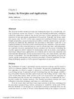
The CPU can be thought of as containing several components connected by
its own internal bus, which is distinct from the memory and address buses of
the system. As shown in Figure 2.6 the CPU contains a program counter (PC),
an arithmetic logic unit (ALU), internal CPU memory–scratch pad memory and
PC
SR
IR
MDR
R1
MAR
Rn
…
Stack

Pointer
Micro
Memory
Control
Unit
Interrupt
Controller
CPU
Address Bus
Data Bus
Collectively known
as the “bus” or
“system bus”
Figure 2.6 Partial, stylized, internal structure of a typical CPU. The internal paths represent
connections to the internal bus structure. The connection to the system bus is shown on
the right.
1
Some of the following discussion in this section is adapted from Computer Architecture: A Mini-
malist Perspective by Gilreath and Laplante [Gilreath03].
30 2 HARDWARE CONSIDERATIONS
micromemory, general registers (labelled ‘R1’ through ‘Rn’), an instruction reg-
ister (IR), and a control unit (CU). In addition, a memory address register (MAR)
holds the address of the memory location to be acted on, and a memory date
register (MDR) holds the data to be written to the MAR or that have been read
from the memory location held in the MAR.
There is an internal clock and other signals used for timing and data transfer,
and other hidden internal registers that are typically found inside the CPU, but
are not shown in Figure 2.6.
2.3.1 Fetch and Execute Cycle
Programs are a sequence of macroinstructions or macrocode. These are stored

in the main memory of the computer in binary form and await execution. The
macroinstructions are sequentially fetched from the main memory location pointed
to by the program counter, and placed in the instruction register.
Each instruction consists of an operation code (opcode) field and zero or more
operand fields. The opcode is typically the starting address of a lower-level pro-
gram stored in micromemory (called a microprogram), and the operand represents
registers, memory, or data to be acted upon by this program.
The control unit decodes the instruction. Decoding involves determining the
location of the program in micromemory and then internally executing this
program, using the ALU and scratch-pad memory to perform any necessary
arithmetic computations. The various control signals and other internal registers
facilitate data transfer, branching, and synchronization.
After executing the instruction, the next macroinstruction is retrieved from
main memory and executed. Certain macroinstructions or external conditions
may cause a nonconsecutive macroinstruction to be executed. This case is dis-
cussed shortly. The process of fetching and executing an instruction is called the
fetch–execute cycle. Even when “idling,” the computer is fetching and execut-
ing an instruction that causes no effective change to the state of the CPU and is
called a no-operation (no-op). Hence, the CPU is constantly active.
2.3.2 Microcontrollers
Not all real-time systems are based on a microprocessor. Some may involve a
mainframe or minicomputers, while others are based on a microcontroller. Very
large real-time systems involving mainframe or minicomputer control are unusual
today unless the system requires tremendous CPU horsepower and does not need
to be mobile (for example, an air traffic control system). But, microcontroller-
based real-time systems abound.
A microcontroller is a computer system that is programmable via microinstruc-
tions (Figure 2.7). Because the complex and time-consuming macroinstruction
decoding process does not occur, program execution tends to be very fast.
Unlike the complex instruction decoding process found in a traditional micro-

processor, the microcontroller directly executes “fine grained” instructions stored
2.3 CENTRAL PROCESSING UNIT 31
Microinstruction
Register
Micromemory
Microinstructions
Microcontrol
Unit
Decoder
External input
Signals
Clock
Figure 2.7 Stylized microcontroller block diagram.
in micromemory. These fine-grained instructions are wider than macroinstruc-
tions (in terms of number of bits) and directly control the internal gates of the
microcontroller hardware. The microcontroller can take direct input from devices
and directly control external output signals. High-level language and tool support
allows for straightforward code development.
2.3.3 Instruction Forms
An instruction set constitutes the language that describes a computer’s function-
ality. It is also a function of the computer’s organization.
2
While an instruction
set reflects differing underlying processor design, all instruction sets have much
in common in terms of specifying functionality.
Instructions in a processor are akin to functions in procedural programming
language in that both take parameters and return a result. Most instructions make
reference to either memory locations, pointers to a memory location, or a regis-
ter.
3

The memory locations eventually referenced contain data that are processed
to produce new data. Hence, any computer processor can be viewed as a machine
for taking data and transforming it, through instructions, into new information.
It is important to distinguish which operand is being referenced in describing
an operation. As in arithmetic, different operations use different terms for the
parameters to distinguish them. For example, addition has addend and augends,
2
Traditionally, the distinction between computer organization and computer architecture is that the
latter involves using only those hardware details that are visible to the programmer, while the former
involves implementation details.
3
An exception to this might be a HALT instruction. However, any other instruction, even those that
are unary, will affect the program counter, accumulator, or a stack location.
32 2 HARDWARE CONSIDERATIONS
subtraction has subtract and and subtrahend, multiplication has multiplicand and
multiplier, and division has dividend and divisor.
In a generic sense, the two terms “operandam” and “operandum” can be used to
deal with any unary or binary operation. The operandam is the first parameter, like
an addend, multiplicand, or dividend. The operandum is the second parameter,
like the augend, multiplier, or divisor. The following formal definitions will be
helpful, as these terms will be used throughout the text.
The defining elements of instructions hint at the varying structures for orga-
nizing information contained within the instruction. In the conventional sense,
instructions can be regarded as an n-tuple, where the n refers to the parameters
of the instruction.
In the following sections, the instruction formats will be described beginning
with the most general to the more specific. The format of an instruction provides
some idea of the processor’s architecture and design. However, note that most
processors use a mix of instruction forms, especially if there is an implicit register.
The following, self-descriptive examples illustrate this point.

2.3.3.1 1-Address and 0-Address Forms Some processors have instruc-
tions that use a single, implicit register called an accumulator as one of the
operands. Other processors have instruction sets organized around an internal
stack in which the operands are found in the two uppermost stack locations
(in the case of binary operations) or in the uppermost location (in the case
of unary operations). These 0-address (or 0-address or stack) architectures can
be found in programmable calculators that are programmed using postfix
notation.
2.3.3.2 2-Address Form A 2-address form is a simplification (or complica-
tion, depending on the point of view) of the 3-address form. The 2-address (or
2-tuple) form means that an architectural decision was made to have the resultant
and operandum as the same. The 2-address instruction is of the form:
op-code operandam, operandum
As a mathematical function, the 2-address would be expressed as:
operandum = op-code(operandam, operandum)
Hence, the resultant is implicitly given as the operandum and stores the result of
the instruction.
The 2-address form simplifies the information provided, and many high-level
language program instructions often are self-referencing, such as the C lan-
guage statement:
i=i+1;
which has the short form:
i++;
2.3 CENTRAL PROCESSING UNIT 33
This operation could be expressed with an ADD instruction in 2-address form as:
ADD 0x01, &i ; 2-address
where &i is the address of the i variable.
4
A 3-address instruction would redun-
dantly state the address of the

i variable twice: as the operandum and as the
resultant as follows:
ADD 0x01, &i, &i ; 3-address
However, not all processor instructions map neatly into 2-address form, so this
form can be inefficient. The 80×86 family of processors, including the Pentium,

use this instruction format.
2.3.3.3 3-Address Form The 3-address instruction is of the form:
op-code operandam, operandum, resultant
This is closer to a mathematical functional form, which would be
resultant = op-code(operandam, operandum)
This form is the most convenient from a programming perspective and leads to
the most compact code.
2.3.4 Core Instructions
In any processor architecture, there are many instructions, some oriented toward
the architecture and others of a more general kind. In fact, all processors share a
core set of common instructions.
There are generally six kinds of instructions. These can be classified as:
ž
Horizontal-bit operation
ž
Vertical-bit operation
ž
Control
ž
Data movement
ž
Mathematical/special processing
ž
Other (processor specific)

The following sections discuss these instruction types in some detail.
2.3.4.1 Horizontal-Bit Operation The horizontal-bit operation is a gener-
alization of the fact that these instructions alter bits within a memory in the
horizontal direction, independent of one another. For example, the third bit in
4
This convention is used throughout the book.
34 2 HARDWARE CONSIDERATIONS
the operands would affect the third bit in the resultant. Usually, these instructions
are the
AND, IOR, XOR, NOT operations.
These operations are often called “logical” operators, but practically speaking,
they are bit operations. Some processors have an instruction to specifically access
and alter bits within a memory word.
2.3.4.2 Vertical-Bit Operation The vertical-bit operation alters a bit within
a memory word in relation to the other bits. These are the rotate-left, rotate-right,
shift-right, and shift-left operations. Often shifting has an implicit bit value on
the left or right, and rotating pivots through a predefined bit, often in a status
register of the processor.
2.3.4.3 Control Both horizontal- and vertical-bit operations can alter a word
within a memory location, but a processor has to alter its state to change flow of
execution and which instructions the processor executes.
5
This is the purpose of
the control instructions, such as compare and jump on a condition. The compare
instruction determines a condition such as equality, inequality, and magnitude.
The jump instruction alters the program counter based upon the condition of the
status register.
Interrupt handling instructions, such as the Intel 80×86’s
CLI, clears the inter-
rupt flag in the status register, or the TRAP in the Motorola 68000 handles

exceptions. Interrupt handling instructions can be viewed as asynchronous control
instructions.
The enable priority interrupt (
EPI) is used to enable interrupts for processing
by the CPU. The disable priority interrupt (
DPI) instruction prevents the CPU
from processing interrupts (i.e., being interrupted). Disabling interrupts does not
remove the interrupt as it is latched; rather, the CPU “holds off” the interrupt
until an
EPI instruction is executed.
Although these systems may have several interrupt signals, assume that the
CPU honors only one interrupt signal. This has the advantage of simplifying the
instruction set and off-loading certain interrupt processing. Such tasks as prioriti-
zation and masking of certain individual interrupts are handled by manipulating
the interrupt controller via memory-mapped I/O or programmed I/O.
Modern microprocessors also provide a number of other instructions specifi-
cally to support the implementation of real-time systems. For example, the Intel
IA-32 family provides
LOCK, HLT,andBTS instructions, among others.
The
LOCK instruction causes the processor’s LOCK# signal to be asserted dur-
ing execution of the accompanying instruction, which turns the instruction into
an atomic (uninterruptible) instruction. Additionally, in a multiprocessor envi-
ronment, the
LOCK# signal ensures that the processor has exclusive use of any
shared memory while the signal is asserted.
The
HLT (halt processor) instruction stops the processor until, for example,
an enabled interrupt or a debug exception is received. This can be useful for
5

If this were not the case, the machine in question would be a calculator, not a computer!
2.3 CENTRAL PROCESSING UNIT 35
debugging purposes in conjunction with a coprocessor (discussed shortly), or for
use with a redundant CPU. In this case, a self-diagnosed faulty CPU could issue
a signal to start the redundant CPU, then halt itself, which can be awakened
if needed.
The
BTS (bit test and set) can be used with a LOCK prefix to allow the instruction
to be executed atomically. The test and set instructions will be discussed later in
conjunction with the implementation of semaphores.
Finally, the IA-32 family provides a read performance-monitoring counter and
read time-stamp counter instructions, which allow an application program to
read the processor’s performance-monitoring and time-stamp counters, respec-
tively. The Pentium 4

processors have eighteen 40-bit performance-monitoring
counters, and the P6

family processors have two 40-bit counters. These counters
can be used to record either the occurrence or duration of events.
2.3.4.4 Mathematical Most applications require that the computer be able to
process data stored in both integer and floating-point representation. While integer
data can usually be stored in 2 or 4 bytes, floating-point quantities typically need
4 or more bytes of memory. This necessarily increases the number of bus cycles
for any instruction requiring floating-point data.
In addition, the microprograms for floating-point instructions are considerably
longer. Combined with the increased number of bus cycles, this means floating-
point instructions always take longer than their integer equivalents. Hence, for
execution speed, instructions with integer operands are always preferred over
instructions with floating-point operands.

Finally, the instruction set must be equipped with instructions to convert integer
data to floating-point and vice versa. These instructions add overhead while pos-
sibly reducing accuracy. Therefore mixed-mode calculations should be avoided
if possible.
The bit operation instructions can create the effects of binary arithmetic, but
it is far more efficient to have the logic gates at the machine hardware level
implement the mathematical operations. This is true especially in floating-point
and dedicated instructions for math operations. Often these operations are the
ADD, SUB, MUL, DIV, as well as more exotic instructions. For example, in the
Pentium, there are built-in instructions for more efficient processing of graphics.
2.3.4.5 Data Movement The I/O movement instructions are used to move
data to and from registers, ports, and memory. Data must be loaded and stored
often. For example in the C language, the assignment statement is
i=c;
As a 2-address instruction, it would be
MOVE &c, &i
Most processors have separate instructions to move data into a register from
memory (
LOAD), and to move data from a register to memory (STORE). The Intel
36 2 HARDWARE CONSIDERATIONS
80×86 has dedicated IN, OUT to move data in and out of the processor through
ports, but it can be considered to be a data movement instruction type.
2.3.4.6 Other Instructions The only other kinds of instructions are those
specific to a particular architecture. For example, the 8086 LOCK instruction pre-
viously discussed. The 68000 has an
ILLEGAL instruction, which does nothing but
generate an exception. Such instructions as
LOCK and ILLEGAL are highly processor
architecture specific, and are rooted in the design requirements of the processor.
2.3.5 Addressing Modes

The addressing modes represent how the parameters or operands for an instruction
are obtained. The addressing of data for a parameter is part of the decoding
process for an instruction (along with decoding the instruction) before execution.
Although some architectures have ten or more possible addressing modes, there
are really three basic types of addressing modes:
ž
Immediate data
ž
Direct memory location
ž
Indirect memory location
Each addressing mode has an equivalent in a higher-level language.
2.3.5.1 Immediate Data Immediate data are constant, and they are found in
the memory location succeeding the instruction. Since the processor does not have
to calculate an address to the data for the instruction, the data are immediately
available. This is the simplest form of operand access. The high-level language
equivalent of the immediate mode is a literal constant within the program code.
2.3.5.2 Direct Memory Location A direct memory location is a variable.
That is, the data are stored at a location in memory, and it is accessed to obtain
the data for the instruction parameter. This is much like a variable in a higher-
level language – the data are referenced by a name, but the name itself is not
the value.
2.3.5.3 Indirect Memory Location An indirect memory location is like a
direct memory location, except that the former does not store the data for the
parameter, it references or “points” to the data. The memory location contains an
address that then refers to a direct memory location. A pointer in the high-level
language is the equivalent in that it references where the actual data are stored
in memory and not, literally, the data.
2.3.5.4 Other Addressing Modes Most modern processors employ com-
binations of the three basic addressing modes to create additional addressing

modes. For example, there is a computed offset mode that uses indirect memory
locations. Another would be a predecrement of a memory location, subtracting
2.3 CENTRAL PROCESSING UNIT 37
one from the address where the data are stored. Different processors will expand
upon these basic addressing modes, depending on how the processor is oriented
to getting and storing the data.
One interesting outcome is that the resultant of an operational instruction can-
not be immediate data; it must be a direct memory location, or indirect memory
location. In 2-address instructions, the destination, or operandum resultant, must
always be a direct or indirect memory location, just as an L-value in a higher-level
language cannot be a literal or named constant.
2.3.6 RISC versus CISC
Complex instruction set computers (CISC) supply relatively sophisticated func-
tions as part of the instruction set. This gives the programmer a variety of
powerful instructions with which to build applications programs and even more
powerful software tools, such as assemblers and compilers. In this way, CISC pro-
cessors seek to reduce the programmer’s coding responsibility, increase execution
speeds, and minimize memory usage.
The CISC is based on the following eight principles:
1. Complex instructions take many different cycles.
2. Any instruction can reference memory.
3. No instructions are pipelined.
4. A microprogram is executed for each native instruction.
5. Instructions are of variable format.
6. There are multiple instructions and addressing modes.
7. There is a single set of registers.
8. Complexity is in the microprogram and hardware.
In addition, program memory savings are realized because implementing com-
plex instructions in high-order language requires many words of main memory.
Finally, functions written in microcode always execute faster than those coded

in the high-order language.
In a reduced instruction set computer (RISC) each instruction takes only one
machine cycle. Classically, RISCs employ little or no microcode. This means that
the instruction-decode procedure can be implemented as a fast combinational
circuit, rather than a complicated microprogram scheme. In addition, reduced
chip complexity allows for more on-chip storage (i.e., general-purpose regis-
ters). Effective use of register direct instructions can decrease unwanted memory
fetch time
The RISC criteria are a complementary set of eight principles to CISC.
These are:
1. Simple instructions taking one clock cycle.
2. LOAD/STORE architecture to reference memory.
3. Highly pipelined design.
38 2 HARDWARE CONSIDERATIONS
4. Instructions executed directly by hardware.
5. Fixed-format instructions.
6. Few instructions and addressing modes.
7. Large multiple-register sets.
8. Complexity handled by the compiler and software.
A RISC processor can be viewed simply as a machine with a small number
of vertical microinstructions, in which programs are directly executed in the
hardware. Without any microcode interpreter, the instruction operations can be
completed in a single microinstruction.
RISC has fewer instructions; hence, more complicated instructions are imple-
mented by composing a sequence of simple instructions. When this is a frequently
used instruction, the compiler’s code generator can use a template of the instruc-
tion sequence of simpler instructions to emit code as if it were that complex
instruction.
RISC needs more memory for the sequences of instructions that form a com-
plex instruction. CISC uses more processor cycles to execute the microinstruc-

tions used to implement the complex macroinstruction within the processor
instruction set.
RISCs have a major advantage in real-time systems in that, in theory, the
average instruction execution time is shorter than for CISCs. The reduced instruc-
tion execution time leads to shorter interrupt latency and thus shorter response
times. Moreover, RISC instruction sets tend to allow compilers to generate faster
code. Because the instruction set is limited, the number of special cases that the
compiler must consider is reduced, thus permitting a larger number of optimiza-
tion approaches.
On the downside, RISC processors are usually associated with caches and elab-
orate multistage pipelines. Generally, these architectural enhancements greatly
improve the average case performance of the processor by reducing the mem-
ory access times for frequently accessed instructions and data. However, in the
worst case, response times are increased because low cache hit ratios and fre-
quent pipeline flushing can degrade performance. But in many real-time systems,
worst-case performance is typically based on very unusual, even pathological,
conditions. Thus, greatly improving average-case performance at the expense of
degraded worst-case performance is usually acceptable.
2.4 MEMORY
An understanding of certain characteristics of memory technologies is important
when designing real-time systems. The most important of these characteristics
is access time, which is the interval between when a datum is requested from a
memory cell and when it is available to the CPU. Memory access times can have
a profound effect on real-time performance and should influence the choice of
instruction modes used, both when coding in assembly language and in the use
of high-order language idioms.
2.4 MEMORY 39
The effective access time depends on the memory type and technology, the
memory layout, and other factors; its method of determination is complicated
and beyond the scope of this book. Other important memory considerations are

power requirements, density (bits per unit area), and cost.
2.4.1 Memory Access
The typical microprocessor bus read cycle embodies the handshaking between
the processor and the main memory store. The time to complete the handshaking
is entirely dependent on the electrical characteristics of the memory device and
the bus (Figure 2.8). Assume the transfer is from the CPU to main memory. The
CPU places the appropriate address information on the address bus and allows
the signal to settle. It then places the appropriate data onto the data bus. The
CPU asserts the DST
6
signal to indicate to the memory device that the address
lines have been set to the address and the data lines to the data to be accessed.
Another signal (not shown) is used to indicate to the memory device whether the
transfer is to be a load (from) or store (to) transfer. The reverse transfer from
memory to the CPU is enacted in exactly the same way.
2.4.2 Memory Technologies
Memory can be volatile (the contents will be lost if power is removed) or non-
volatile (the contents are preserved upon removing power). In addition there
Time
Data
DST
Clock
Address
Figure 2.8 Illustration of the clock-synchronized memory-transfer process between a device
and the CPU. The symbols ‘‘<>’’ shown in the data and address signals indicates that multiple
lines are involved during this period in the transfer.
6
The symbol names here are typical and will vary significantly from one system to another.
40 2 HARDWARE CONSIDERATIONS
is RAM which is both readable and writeable, and ROM. Within these two

groups are many different classes of memories. Only the more important ones
will be discussed.
RAM memories may be either dynamic or static, and are denoted DRAM and
SRAM, respectively. DRAM uses a capacitive charge to store logic 1s and 0s, and
must be refreshed periodically due to capacitive discharge. SRAMs do not suffer
from discharge problems and therefore do not need to be refreshed. SRAMs are
typically faster and require less power than DRAMs, but are more expensive.
2.4.2.1 Ferrite Core More for historical interest than a practical matter, con-
sider ferrite core, a type of nonvolatile static RAM that replaced memories based
on vacuum tubes in the early 1950s. Core memory consists of a doughnut-shaped
magnet through which a thin drive line passes.
In a core-memory cell, the direction of flow of current through the drive lines
establishes either a clockwise or counterclockwise magnetic flux through the
doughnut that corresponds to either logic 1 or logic 0. A sense line is used to
“read’ the memory (Figure 2.9). When a current is passed through the drive line,
a pulse is generated (or not) in the sense line, depending on the orientation of
the magnetic flux.
Core memories are slow (10-microsecond access), bulky, and consume lots of
power. Although they have been introduced here for historical interest, they do
have one practical advantage – they cannot be upset by electrostatic discharge or
by a charged particle in space. This consideration is important in the reliability
of space-borne and military real-time systems. In addition, the new ferroelectric
memories are descendents of this type of technology.
2.4.2.2 Semiconductor Memory RAM devices can be constructed from
semiconductor materials in a variety of ways. The basic one-bit cells are then
configured in an array to form the memory store. Both static and dynamic RAM
can be constructed from several types of semiconductor materials and designs.
Drive Line
Sense Line
Magnetic Flux

Figure 2.9 A core-memory element. The figure is approximately 15 times larger than
actual size.
2.4 MEMORY 41
Static memories rely on bipolar logic to represent ones and zeros. Dynamic RAMs
rely on capacitive charges, which need to be refreshed regularly due to charge
leakage. Typically, dynamic memories require less power and are denser than
static ones; however, they are much slower because of the need to refresh them.
A SRAM with a battery back up is referred to as an NVRAM (nonvolatile RAM).
The required refresh of the dynamic RAM is accomplished by accessing each
row in memory by setting the row address strobe (RAS) signal without the need
to activate the column address strobe (CAS) signals. The RAM refresh can occur
at a regular rate (e.g., 4 milliseconds) or in one burst.
A significant amount of bus activity can be held off during the dynamic refresh,
and this must be taken into account when calculating instruction execution time
(and hence system performance). When a memory access must wait for a DRAM
refresh to be completed, cycle stealing occurs, that is, the CPU is stalled until
the memory cycle completes. If burst mode is used to refresh the DRAM, then
the timing of critical regions may be adversely affected when the entire memory
is refreshed simultaneously.
Depending on the materials used and the configuration, access times of 15 nano-
seconds or better can be obtained for static semiconductor RAM.
2.4.2.3 Fusible Link Fusible-link ROMs are a type of nonvolatile memory.
These one-time programmable memories consist of an array of paths to ground or
“fusible links.” During programming these fuses are shorted or fused to represent
either 1s or 0s, thus embedding the program into the memory. Just as fusible-link
memories cannot be reprogrammed, they cannot be accidentally altered. They are
fast and can achieve access time of around 50 nanoseconds, though they are not
very dense.
Fusible-link ROM is used to store program instructions and data that are not to
be altered and that require a level of immutability, such as in hardened military

applications.
2.4.2.4 Ultraviolet ROM Ultraviolet ROM (UVROM) is a type of non-
volatile programmable ROM (PROM), with the special feature that it can be
reprogrammed a limited number of times. For reprogramming, the memory is
first erased by exposing the chip to high-intensity ultraviolet light. This repro-
grammability, however render UVROMS susceptible to upset.
UVROM is typically used for the storage of program and fixed constants.
UVROMs have access times similar to those of fusible-link PROMs.
2.4.2.5 Electronically Erasable PROM Electronically erasable PROM
(EEPROM) is another type of PROM with the special feature that it can be
reprogrammed in situ, without the need for a special programming device (as in
UVROM or fusible-link PROM). These memories are erased by toggling signals
on the chip, which can be accomplished under program control.
EEPROMs are used for long-term storage of variable information. For example,
in embedded applications, “black-box” recorder information from diagnostic tests
might be written to EEPROM for postmission analysis.
42 2 HARDWARE CONSIDERATIONS
These memories are slower than other types of PROMs (50–200 nanosecond
access times), limited rewrite cycles (e.g., 10,000), and have higher power require-
ments (e.g., 12 volts).
2.4.2.6 Flash Memory Flash memory is another type of rewritable PROM
that uses a single transistor per bit, whereas EEPROM uses two transistors per
bit. Hence, flash memory is more cost effective and denser then EEPROM. Read
times for flash memory are fast, 20 to 30 nanoseconds, but write speeds are quite
slow – up to 1 microsecond. Another disadvantage of flash memory is that it
can be written to and erased about 100,000 times, whereas EEPROM is approxi-
mately 1 million. Another disadvantage is that flash memory requires rather high
voltages: 12 V to write; 2 V to read. Finally, flash memory can only be written
to in blocks of size 8–128 kilobytes at a time.
This technology is finding its way into commercial electronics applications,

but it is expected to appear increasingly in embedded real-time applications.
2.4.2.7 Ferroelectric Random-Access Memory An emerging technol-
ogy, ferroelectric RAM relies on a capacitor employing a special insulating
material. Data are represented by the orientation of the ferroelectric domains
in the insulting material, much like the old ferrite-core memories. This similar-
ity also extends to relative immunity to upset. Currently, ferroelectric RAM is
available in arrays of up to 64 megabytes with read/write 40 nanosecond access
time and 1.5/1.5 read/write voltage
2.4.3 Memory Hierarchy
Primary and secondary memory storage forms a hierarchy involving access time,
storage density, cost, and other factors. Clearly, the fastest possible memory is
desired in real-time systems, but cost control generally dictates that the fastest
affordable technology is used as required. In order of fastest to slowest, and
considering cost, memory should be assigned as follows:
1. Internal CPU memory
2. Registers
3. Cache
4. Main memory
5. Memory on board external devices
Selection of the appropriate technology is a systems design issue. Table 2.1
summarizes the previously discussed memory technologies and some appropriate
associations with the memory hierarchy.
Note that these numbers vary widely depending on many factors, such as
manufacturer, model and cost, and change frequently. These figures are given
for relative comparison purposes only.
2.4 MEMORY 43
Table 2.1 A summary of memory technologies
Memory Type Typical Access
Time
Density Typical Applications

DRAM 50–100 ns 64 Mbytes Main memory
SRAM 10 ns 1 Mbyte µmemory, cache, fast
RAM
UVROM 50 ns 32 Mbytes Code and data storage
Fusible-link PROM 50 ns 32 Mbytes Code and data storage
EEPROM 50–200 ns 1 Mbyte Persistent storage of
variable data
Flash 20–30 ns
(read) 1 µs
(write)
64 Mbytes Code and data storage
Ferroelectric RAM 40 ns 64 Mbytes Various
Ferrite core 10 ms 2 kbytes or
less
None, possibly
ultrahardened
nonvolatile memory
2.4.4 Memory Organization
To the real-time systems engineer, particularly when writing code, the kind of
memory and layout is of particular interest. Consider, for example, an embed-
ded processor that supports a 32-bit address memory organized, as shown in
Figure 2.10. Of course, the starting and ending addresses are entirely imagi-
nary, but could be representative of a particular embedded system. For example,
such a map might be consistent with the memory organization of the inertial
measurement system.
The executable program resides in memory addresses 00000000 through
E0000000 hexadecimal in some sort of programmable-only ROM, such as fusible
link. It is useful to have the program in immutable memory so that an accidental
write to this region will not catastrophically alter the program. Other data, possi-
bly related to factory settings and tuned system parameters, are stored at locations

E000001 through E0000F00 in EPROM, which can be rewritten only when the
system is not in operation. Locations E0000F01 through FFC00000 are RAM
memory used for the run-time stack, memory heap, and any other transient data
storage. Addresses FFC00001 through FFFFE00 are fixed system parameters that
might need to be rewritten under program control, for example, calibration con-
stants determined during some kind of diagnostic or initialization mode. During
44 2 HARDWARE CONSIDERATIONS
FFFFFFFF
FFFFFF00
FFFFFE00
FFC00000
DMA
Memory-mapped I/O
E0000F00
E0000000
Devices
Devices
Calibration Constants
Stack, Heap, Variables
Fixed Data
Program
00000000
EEPROM
RAM
EPROM
PROM
Figure 2.10 Typical memory map showing designated regions. (Not to scale.).
run time, diagnostic information or black box data might be stored here. These
data are written to the nonvolatile memory rather than to RAM so that they are
available after the system is shut down (or fails) for analysis. Finally, locations

FFFFE00 through FFFFFFFF contain addresses associated with devices that are
accessed either through DMA or memory-mapped I/O.
2.5 INPUT/OUTPUT
In real-time systems the input devices are sensors, transducers, steering mech-
anisms, and so forth. Output devices are typically actuators, switches, and dis-
play devices.
Input and output are accomplished through one of three different methods:
programmed I/O, memory-mapped I/O, or direct memory address (DMA). Each
method has advantages and disadvantages with respect to real-time performance,
cost, and ease of implementation.
2.5.1 Programmed Input/Output
In programmed I/O, special data-movement instructions are used to transfer data
to and from the CPU. An
IN instruction will transfer data from a specified I/O
device into a specified CPU register. An
OUT instruction will output from a
register to some I/O device. Normally, the identity of the operative CPU register
2.5 INPUT/OUTPUT 45
is embedded in the instruction code. Both the IN and OUT instructions require the
efforts of the CPU, and thus cost time that could impact real-time performance.
For example, a computer system is used to control the speed of a motor. An
output port is connected to the motor, and a signed integer is written to the port to
set the motor speed. The computer is configured so that when an
OUT instruction
is executed, the contents of register 1 are placed on the data bus and sent to
the I/O port at the address contained in register 2. The following code fragment
allows the program to set the motor speed.
7
LOAD R1 &speed ;motor speed into register 1
LOAD R2 &motoraddress ;address of motor control into register 2

OUT ;output from register 1 to the memory-mapped I/O
;port address contained in register 2
2.5.2 Direct Memory Access
In DMA, access to the computer’s memory is given to other devices in the system
without CPU intervention. That is, information is deposited directly into main
memory by the external device. Here a DMA controller is required (Figure 2.11)
unless the DMA circuitry is integrated into the CPU. Because CPU participation
is not required, data transfer is fast.
The DMA controller prevents collisions by requiring each device to issue a
DMA request signal (DMARQ) that will be acknowledged with a DMA acknowl-
edge signal (DMACK). Until the DMACK signal is given to the requesting
device, its connection to the main bus remains in a tristate condition. Any device
that is tristated cannot affect the data on the memory data lines. Once the DMACK
CPU Memory
Data and
Address
Buses
DMA
Controller
I/O
Device
DMARQ
DMACK
Data and Address
Buses
Bus Grant
Read/Write
Line
Figure 2.11 DMA circuitry where an external controller is used. This functionality can also be
integrated on-chip with the CPU.

7
So, for example, “R1” is register number 1.
46 2 HARDWARE CONSIDERATIONS
Time
Data
DST
Clock
Address
DMARQ
DMACK
Figure 2.12 The DMA timing process. The sequence is: request transfer (DMARQ high),
receive acknowledgment (DMACK high), place data on bus, and indicate data are present on
bus (DST high). The signal height indicates voltage high/low.
is given to the requesting device, its memory bus lines become active, and data
transfer occurs, as with the CPU (Figure 2.12).
The CPU is prevented from performing a data transfer during DMA through
the use of a signal called a bus grant. Until the bus grant signal is given by the
controller, no other device can obtain the bus. The DMA controller is responsible
for assuring that only one device can place data on the bus at any one time
through bus arbitration. If two or more devices attempt to gain control of the bus
simultaneously, bus contention occurs. When a device already has control of the
bus and another obtains access, an undesirable occurrence (a collision) occurs.
The device requests control of the bus by signaling the controller via the
DMARQ signal. Once the DMACK signal is asserted by the controller, the device
can place (or access) data to/from the bus (which is indicated by another signal,
typically denoted DST).
Without the bus grant (DMACK) from the DMA controller, the normal CPU
data-transfer processes cannot proceed. At this point, the CPU can proceed with
non-bus-related activities (e.g., the execution phase of an arithmetic instruction)
until it receives the bus grant, or until it gives up (after some predetermined time)

and issues a bus time-out signal. Because of its speed, DMA is often the best
method for input and output for real-time systems.
2.5.3 Memory-Mapped Input/Output
Memory-mapped I/O provides a data-transfer mechanism that is convenient be-
cause it does not require the use of special CPU I/O instructions. In memory-
mapped I/O certain designated locations of memory appear as virtual I/O ports
2.5 INPUT/OUTPUT 47
Data and
Address
Buses
CPU
I/O
I/O
Memory
Address
Decoder
Data and
Address
Buses
Figure 2.13 Memory-mapped I/O circuitry.
(Figure 2.13). For example, consider the control of the speed of a stepping motor.
If it were to be implemented via memory-mapped I/O, the required assembly
language code might look like the following:
LOAD R1 &speed ;motor speed into register 1
STORE R1 &motoraddress ;store to address of motor control
where speed is a bit-mapped variable and motoraddress is a memory-mapped
location.
In many computer systems, the video display is updated via memory-mapped
I/O. For example, suppose that a display consists of a 24 row by 80 column array
(a total of 1920 cells). Each screen cell is associated with a specific location in

memory. To update the screen, characters are stored on the address assigned to
that cell on the screen.
Input from an appropriate memory-mapped location involves executing a
LOAD
instruction on a pseudomemory location connected to an input device.
2.5.3.1 Bit Maps A bit map describes a view of a set of devices that are
accessed by a single (discrete) signal and organized into a word of memory for
convenient access either by DMA or memory-mapped addressing. Figure 2.14
Set Indicator Light, On = 1
Motor Control, 4 bits representing 16 speedsOther Devices
11101010
Figure 2.14 Bit map showing mappings between specific bits and the respective devices in
a memory-mapped word.
48 2 HARDWARE CONSIDERATIONS
illustrates a typical bit map for a set of output devices. Each bit in the bit map is
associated with a particular device. For example, in the figure the high-order bit
is associated with a display light. When the bit is set to one, it indicates that the
indicator light is on. The low-order four bits indicate the settings for a 16-speed
stepping motor. Other devices are associated with the remaining bits.
Bit maps can represent either output states, that is, the desired state of the
device, or an indication of the current state of the device in questions, that is, it
is an input or an output.
2.5.4 Interrupts
An interrupt is a hardware signal that initiates an event. Interrupts can be initiated
by external devices, or internally if the CPU is has this capability. External
interrupts are caused by other devices (e.g., clocks and switches), and in most
operating systems such interrupts are required for scheduling. Internal interrupts,
or traps, are generated by execution exceptions, such as a divide-by-zero. Traps
do not use external hardware signals; rather, the exceptional conditions are dealt
with through branching in the microcode. Some CPUs can generate true external

interrupts, however.
2.5.4.1 Instruction Support for Interrupts Processors provide two instruc-
tions, one to enable or turn on interrupts
EPI, and another to disable or turn
them off (
DPI). These are atomic instructions that are used for many purposes,
including buffering, within interrupt handlers, and during parameter passing.
2.5.4.2 Internal CPU Handling of Interrupts Upon receipt of the interrupt
signal, the processor completes the instruction that is currently being executed.
Next, the contents of the program counter are saved to a designated memory
location called the interrupt return location. In many cases, the CPU “flag” or
condition status register (SR) is also saved so that any information about the
previous instruction (for example, a test instruction whose result would indicate
that a branch is required) is also saved. The contents of a memory location called
the interrupt-handler location are loaded into the program counter. Execution then
proceeds with the special code stored at this location, called the interrupt handler.
This process is outlined in Figure 2.15.
Processors that are used in embedded systems are equipped with circuitry that
enables them to handle more than one interrupt in a prioritized fashion. The
overall scheme is depicted in Figure 2.16.
Upon receipt of interrupt i, the circuitry determines whether the interrupt is
allowable given the current status and mask register contents. If the interrupt is
allowed, the CPU completes the current instruction and then saves the program
counter in interrupt-return location i. The program counter is then loaded with
the contents of interrupt-handler location i. In some architectures, however, the
return address is saved in the system stack, which allows for easy return from a
sequence of interrupts by popping the stack. In any case, the code at the address
there is used to service the interrupt.
2.5 INPUT/OUTPUT 49
Interrupt

Signal
Program
Counter
CPU
Interrupt-Return
Location
Interrupt-Handler
Location
Memory
2.
1.
3.
Figure 2.15 Sketch of the interrupt-handling process in a single-interrupt system. Step 1:
finish the currently executing macroinstruction. Step 2: save the contents of the program
counter to the interrupt-return location. Step 3: load the address held in the interrupt-handler
location into the program counter. Resume the fetch and execute sequence.
Interrupt
Signal 1
Interrupt
Signal
n
. . .
1.
3.
2.
1
1
i
n
Interrupt-Handler Locations

i
n
Interrupt-Return Locations
Program
Counter
Figure 2.16 The interrupt-handling process in a multiple-interrupt system. Step 1: complete
the currently executing instruction. Step 2: save the contents of the program counter to
interrupt-return location i. Step 3: load the address held in interrupt-handler location i into the
program counter. Resume the fetch–execute cycle.
50 2 HARDWARE CONSIDERATIONS
To return from the interrupt, the saved contents of the program counter at the
time of interruption are reloaded into the program counter and the usual fetch
and execute sequence is resumed.
Interrupt-driven I/O is simply a variation of program I/O, memory-mapped
I/O, or DMA, in which an interrupt is used to signal that an I/O transfer has
completed or needs to be initiated via one of the three mechanisms.
2.5.4.3 Programmable Interrupt Controller Not all CPUs have the built-
in capability to prioritize and handle multiple interrupts. An external interrupt-
controller device can be used to enable a CPU with a single-interrupt input to
handle interrupts from several sources. These devices have the ability to pri-
oritize and mask interrupts of different priority levels. The circuitry on board
these devices is quite similar to that used by processors that can handle multiple
interrupts (Figure 2.17).
This additional hardware includes special registers, such as the interrupt vector,
status register, and mask register. The interrupt vector contains the identity of the
highest-priority interrupt request; the status register contains the value of the low-
est interrupt that will currently be honored; and the mask register contains a bit
map that either enables or disables specific interrupts. Another specialized register
is the interrupt register, which contains a bit map of all pending (latched) inter-
rupts. Programmable interrupt controllers (PICs) can support a large number of

devices. For example, the Intel 82093AA I/O Advanced Programmable Interrupt
Controller supports 24 programmable interrupts. Each can be independently set
to be edge or level triggered, depending on the needs of the attached device.
Control Logic
Interrupt
Vector
Priority
Register
Interrupt
Register
Status
Register
Mask
Register
Interrupt Signal
to CPU
Data Bus
Buffer
Interrupts
Data Bus
Figure 2.17 A programmable interrupt controller (PIC). The registers-interrupt, priority, vector,
status, and mask-serve the same functions previously described for the interrupt control circuitry
on board a similarly equipped CPU.
2.5 INPUT/OUTPUT 51
CPU
Interrupt-Return
Location
Interrupt-Handler
Location
Memory

2.
1.
3.
Interrupt
Controller
.
.
.
Interrupt
Signals
Interrupt
Signal
Program
Counter
Figure 2.18 Handling multiple interrupts with an external interrupt controller. Step 1: finish
the currently executing instruction. Step 2: save the contents of the program counter into the
interrupt-return location. Step 3: load the address held in the interrupt-handler location into
the program counter. Resume the fetch and execute cycle. The interrupt-handler routine will
interrogate the PIC and take the appropriate action.
When configured as in Figure 2.18, a single-interrupt CPU in conjunction with
an interrupt controller can handle multiple interrupts.
The following scenario illustrates the complexity of writing interrupt-handler
software, and points out a subtle problem that can arise.
An interrupt handler executes upon receipt of a certain interrupt signal that
is level triggered. The first instruction of the routine is to clear the interrupt by
strobing bit 1 of the interrupt clear signal. Here,
intclr is a memory-mapped
location whose least significant bit is connected with the clear interrupt signal.
Successively storing 0, 1, and 0 serves to strobe the bit.
Although the interrupt controller automatically disables other interrupts on

receipt of an interrupt, the code immediately reenables them to detect spuri-
ous ones. The following code fragment illustrates this process for a 2-address
architecture pseudoassembly code:
LOAD R1,0 ;load register 1 with the constant value 0
LOAD R2,1 ;load register 2 with the constant value 1
STORE R1, &intclr ;set clear interrupt signal low
STORE R2, &intclr ;set clear interrupt signal high
STORE R1, &intclr ;set clear interrupt signal low
EPI ;enable interrupt
The timing sequence is illustrated in Figure 2.19.
Note, however, that a problem could occur if the interrupt is cleared too
quickly. Suppose that the clear,
LOAD,andSTORE instructions take 0.75 micro-
second, but the interrupt pulse is 4 microseconds long. If the clear interrupt
instruction is executed immediately upon receipt of the interrupt, a total of
52 2 HARDWARE CONSIDERATIONS
Time
Clear
Interrupt
Interrupt
Signal
Enable
Interrupt
Real Interrupt
Occurs
False Interrupt
Occurs
Figure 2.19 Timing sequence for interrupt clearing that could lead to a problem.
3 microseconds will elapse. Since the interrupt signal is still present, when inter-
rupts are enabled, a spurious interrupt will be caused. This problem is insidious,

because most of the time software and hard delays hold off the interrupt-handler
routine until long after the interrupt signal has latched and gone away. It often
manifests itself when the CPU has been replaced by a faster one.
2.5.4.4 Interfacing Devices to the CPU via Interrupts Most processors
have at least one pin designated as an interrupt input pin, and many peripheral-
device controller chips have a pin designated as an interrupt output pin. The
interrupt request line (IRL) from the peripheral controller chip connects to an
interrupt input pin on the CPU (Figure 2.20).
When the controller needs servicing from the CPU, the controller sends a
signal down the IRL. In response, the CPU begins executing the interrupt service
routine associated with the device in the manner previously described. When the
CPU reads data from (or writes data to) the peripheral controller chip, the CPU
first places the controller’s address on the address bus. The decode logic interprets
that address and enables I/O to the controller through the device-select line.
Suppose now that the system is equipped with a PIC chip that can handle
multiple peripheral controllers and can support 8 or 16 peripheral devices. The
interrupt request lines from the peripheral controllers connect to the interrupt
controller chip. Figure 2.21 depicts a hardware arrangement to handle multiple
peripheral devices.
2.5 INPUT/OUTPUT 53
Address
Decode
Logic
Peripheral
Controller
CPU
IRL
Address Bus
Device Select Line
Data Bus

Figure 2.20 A single peripheral controller. IRL is the interrupt request line.
Peripheral
Controller 1
Interrupt
Controller
Chip
CPU
Address
Decode
Logic
Peripheral
Controller 2
IRL
IRL
IAck
Address Bus
Device Select Line
Data Bus
Figure 2.21 Several peripheral controllers connected to the CPU via a PIC. Notice that the
devices share the common data bus, which is facilitated by tristating, nonactive devices via the
device-select lines.
The interrupt controller chip demultiplexes by combining two or more IRLs
into one IRL that connects to the CPU. Interrupt controllers can be cascaded
in master–slave fashion. When an interrupt arrives at one of the slave interrupt
controllers, the slave interrupts the master controller, which in turn interrupts the
CPU. In this way, the interrupt hardware can be extended.