ADVANCED MECHANICS OF COMPOSITE MATERIALS Episode 2 ppsx

22 Advanced mechanics of composite materials
the mechanical properties of metal matrix composites are controlled by the matrix to a
considerably larger extent, though the fibers still provide the major contribution to the
strength and stiffness of the material.
The next step in the development of composite materials that can be treated as matrix
materials reinforced with fibers rather than fibers bonded with matrix (which is the case
for polymeric composites) is associated with ceramic matrix composites possessing very
high thermal resistance. The stiffnesses of the fibers which are usually metal (steel,
tungsten, molybdenum, niobium), carbon, boron, or ceramic (SiC, Al
2
O
3
) and ceramic
matrices (oxides, carbides, nitrides, borides, and silicides) are not very different, and
the fibers do not carry the main fraction of the load in ceramic composites. The func-
tion of the fibers is to provide strength and mainly toughness (resistance to cracks) of
the composite, because non-reinforced ceramic materials are very brittle. Ceramic com-
posites can operate under very high temperatures depending on the melting temperature
of the matrix that varies from 1200 to 3500
◦
C. Naturally, the higher the temperature,
the more complicated is the manufacturing process. The main shortcoming of ceramic
composites is associated with a low ultimate tensile elongation of the ceramic matrix
resulting in cracks appearing in the matrix under relatively low tensile stress applied to the
material.
An outstanding combination of high mechanical characteristics and temperature resis-
tance is demonstrated by carbon–carbon composites in which both components – fibers
and matrix are made from one and the same material but with different structure. A carbon
matrix is formed as a result of carbonization of an organic resin (phenolic and furfural resin
or pitch) with which carbon fibers are impregnated, or of chemical vapor deposition of
pyrolitic carbon from a hydrocarbon gas. In an inert atmosphere or in a vacuum, carbon–

carbon composites can withstand very high temperatures (more than 3000
◦
C). Moreover,
their strength increases under heating up to 2200
◦
C while the modulus degrades at tem-
peratures above 1400
◦
C. However in an oxygen atmosphere, they oxidize and sublime
at relatively low temperatures (about 600
◦
C). To use carbon–carbon composite parts in
an oxidizing atmosphere, they must have protective coatings, made usually from silicon
carbide. Manufacturing of carbon–carbon parts is a very energy- and time-consuming
process. To convert an initial carbon–phenolic composite into carbon–carbon, it should
receive a thermal treatment at 250
◦
C for 150h, carbonization at about 800
◦
C for about
100 h and several cycles of densification (one-stage pyrolisis results in high porosity of the
material) each including impregnation with resin, curing, and carbonization. To refine the
material structure and to provide oxidation resistance, a further high-temperature graphi-
tization at 2700
◦
C and coating (at 1650
◦
C) can be required. Vapor deposition of pyrolitic
carbon is also a time-consuming process performed at 900–1200
◦

C under a pressure of
150–2000 kPa.
1.2.3. Processing
Composite materials do not exist apart from composite structures and are formed while
the structure is fabricated. Being a heterogeneous media, a composite material has two
levels of heterogeneity. The first level represents a microheterogeneity induced by at
Chapter 1. Introduction 23
least two phases (fibers and matrix) that form the material microstructure. At the second
level the material is characterized by a macroheterogeneity caused by the laminated or
more complicated macrostructure of the material which consists usually of a set of layers
with different orientations. A number of technologies have been developed by now to
manufacture composite structures. All these technologies involve two basic processes
during which material microstructure and macrostructure are formed.
The first basic process yielding material microstructure involves the application of a
matrix material to the fibers. The simplest way to do it, normally utilized in the manufac-
turing of composites with thermosetting polymeric matrices, is a direct impregnation of
tows, yarns, fabrics, or more complicated fibrous structures with liquid resins. Thermo-
setting resin has relatively low viscosity (10–100 Pa s), which can be controlled using
solvents or heating, and good wetting ability for the majority of fibers. There exist two
versions of this process. According to the so-called ‘wet’ process, impregnated fibrous
material (tows, fabrics, etc.) is used to fabricate composite parts directly, without any
additional treatment or interruption of the process. In contrast to that, in ‘dry’ or ‘prepreg’
processes, impregnated fibrous material is dried (not cured) and thus preimpregnated tapes
obtained (prepregs) are stored for further utilization (usually under low temperature to pre-
vent uncontrolled premature polymerization of the resin). An example of a machine for
making prepregs is shown in Fig. 1.16. Both processes, having similar advantages and
shortcomings, are widely used for composites with thermosetting matrices. For thermo-
plastic matrices, application of direct impregnation (‘wet’ processing) is limited by the
relatively high viscosity (about 10
12

Pa s) of thermoplastic polymer solutions or melts. For
this reason, ‘prepreg’ processes with preliminary fabricated tapes or sheets in which fibers
are already combined with the thermoplastic matrix are used to manufacture composite
parts. There also exist other processes that involve application of heat and pressure to
hybrid materials including reinforcing fibers and a thermoplastic polymer in the form of
powder, films, or fibers. A promising process (called fibrous technology) utilizes tows,
tapes, or fabrics with two types of fibers – reinforcing and thermoplastic. Under heat and
pressure, thermoplastic fibers melt and form the matrix of the composite material. Metal
and ceramic matrices are applied to fibers by means of casting, diffusion welding, chem-
ical deposition, plasma spraying, processing by compression molding or with the aid of
powder metallurgy methods.
The second basic process provides the proper macrostructure of a composite material
corresponding to the loading and operational conditions of the composite part that is
fabricated. There exist three main types of material macrostructure – linear structure
which is appropriate for bars, profiles, and beams, plane laminated structure suitable for
thin-walled plates and shells, and spatial structure which is necessary for thick-walled and
bulk solid composite parts.
A linear structure is formed by pultrusion, table rolling, or braiding and provides high
strength and stiffness in one direction coinciding with the axis of a bar, profile, or a beam.
Pultrusion results in a unidirectionally reinforced composite profile made by pulling a bun-
dle of fibers impregnated with resin through a heated die to cure the resin and, to provide
the desired shape of the profile cross section. Profiles made by pultrusion and braiding
are shown in Fig. 1.17. Table rolling is used to fabricate small diameter tapered tubular
bars (e.g., ski poles or fishing rods) by rolling preimpregnated fiber tapes in the form of
24 Advanced mechanics of composite materials
Fig. 1.16. Machine making a prepreg from fiberglass fabric and epoxy resin. Courtesy of CRISM.
Chapter 1. Introduction 25
Fig. 1.17. Composite profiles made by pultrusion and braiding. Courtesy of CRISM.
flags around the metal mandrel which is pulled out of the composite bar after the resin
is cured. Fibers in the flags are usually oriented along the bar axis or at an angle to the

axis thus providing more complicated reinforcement than the unidirectional one typical of
pultrusion. Even more complicated fiber placement with orientation angle varying from
5to85
◦
along the bar axis can be achieved using two-dimensional (2D) braiding which
results in a textile material structure consisting of two layers of yarns or tows interlaced
with each other while they are wound onto the mandrel.
A plane-laminated structure consists of a set of composite layers providing the necessary
stiffness and strength in at least two orthogonal directions in the plane of the laminate.
Such a plane structure would be formed by hand or machine lay-up, fiber placement, or
filament winding.
Lay-up and fiber placement technology provides fabrication of thin-walled composite
parts of practically arbitrary shape by hand or automated placing of preimpregnated uni-
directional or fabric tapes onto a mold. Layers with different fiber orientations (and even
with different fibers) are combined to result in the laminated composite material exhibit-
ing the desired strength and stiffness in given directions. Lay-up processes are usually
accompanied by pressure applied to compact the material and to remove entrapped air.
Depending on the required quality of the material, as well as on the shape and dimensions
of a manufactured composite part, compacting pressure can be provided by rolling or vac-
uum bags, in autoclaves, or by compression molding. A catamaran yacht (length 9.2m,
width 6.8 m, tonnage 2.2 tons) made from carbon–epoxy composite by hand lay-up is
shown in Fig. 1.18.
Filament winding is an efficient automated process of placing impregnated tows or tapes
onto a rotating mandrel (Fig. 1.19) that is removed after curing of the composite material.
Varying the winding angle, it is possible to control the material strength and stiffness within
the layer and through the thickness of the laminate. Winding of a pressure vessel is shown
in Fig. 1.20. Preliminary tension applied to the tows in the process of winding induces
26 Advanced mechanics of composite materials
Fig. 1.18. Catamaran yacht Ivan-30 made from carbon–epoxy composite by hand lay-up. Courtesy of CRISM.
Chapter 1. Introduction 27

Fig. 1.19. Manufacturing of a pipe by circumferential winding of preimpregnated fiberglass fabric. Courtesy
of CRISM.
Fig. 1.20. Geodesic winding of a pressure vessel.
28 Advanced mechanics of composite materials
Fig. 1.21. A body of a small plane made by filament winding. Courtesy of CRISM.
pressure between the layers providing compaction of the material. Filament winding is the
most advantageous in manufacturing thin-walled shells of revolution though it can also
be used in building composite structures with more complicated shapes (Fig. 1.21).
Spatial macrostructure of the composite material that is specific for thick-walled and
solid members requiring fiber reinforcement in at least three directions (not lying in one
plane) can be formed by 3D braiding (with three interlaced yarns) or using such tex-
tile processes as weaving, knitting, or stitching. Spatial (3D, 4D, etc.) structures used in
carbon–carbon technology are assembled from thin carbon composite rods fixed in dif-
ferent directions. Such a structure that is prepared for carbonization and deposition of
a carbon matrix is shown in Fig. 1.22.
There are two specific manufacturing procedures that have an inverse sequence of the
basic processes described above, i.e., first, the macrostructure of the material is formed
and then the matrix is applied to fibers.
The first of these procedures is the aforementioned carbon–carbon technology that
involves chemical vapor deposition of a pyrolitic carbon matrix on preliminary assembled
and sometimes rather complicated structures made from dry carbon fabric. A carbon–
carbon shell made by this method is shown in Fig. 1.23.
The second procedure is the well-known resin transfer molding. Fabrication of a com-
posite part starts with a preform that is assembled in the internal cavity of a mold from dry
fabrics, tows, yarns, etc., and forms the macrostructure of a composite part. The shape of
this part is governed by the shape of the mold cavity into which liquid resin is transferred
under pressure through injection ports.
The basic processes described above are always accompanied by a thermal treatment
resulting in the solidification of the matrix. Heating is applied to cure thermosetting resins,
cooling is used to transfer thermoplastic, metal, and ceramic matrices to a solid phase,

Chapter 1. Introduction 29
Fig. 1.22. A 4D spatial structure. Courtesy of CRISM.
Fig. 1.23. A carbon–carbon conical shell. Courtesy of CRISM.
30 Advanced mechanics of composite materials
whereas a carbon matrix is made by pyrolisis. The final stages of the manufacturing
procedure involve removal of mandrels, molds, or other tooling and machining of a
composite part.
The fabrication processes are described in more detail elsewhere (e.g., Peters, 1998).
1.3. References
Bogdanovich, A.E. and Pastore, C.M. (1996). Mechanics of Textile and Laminated Composites. Chapman &
Hall, London.
Chou, T.W. and Ko, F.K. (1989). Textile Structural Composites (T.W. Chou and F.K. Ko eds.). Elsevier, NewYork.
Fukuda, H., Yakushiji, M. and Wada, A. (1997). Loop test for the strength of monofilaments. In Proc. 11th
Int. Conf. on Comp. Mat. (ICCM-11), Vol. 5, Textile Composites and Characterization (M.L. Scott ed.).
Woodhead Publishing Ltd., Gold Coast, Australia, pp. 886–892.
Goodey, W.J. (1946). Stress Diffusion Problems. Aircraft Eng. June, 195–198; July, 227–234; August, 271–276;
September, 313–316; October, 343–346; November, 385–389.
Karpinos, D.M. (1985). Composite Materials. Handbook (D.M. Karpinos ed.). Naukova Dumka, Kiev
(in Russian).
Peters, S.T. (1998). Handbook of Composites, 2nd edn. (S.T. Peters ed.). Chapman & Hall, London.
Tarnopol’skii, Yu.M., Zhigun, I.G. and Polyakov, V.A. (1992). Spatially Reinforced Composites. Technomic,
Pennsylvania.
Vasiliev, V.V. and Tarnopol’skii, Yu.M. (1990). Composite Materials. Handbook (V.V. Vasiliev and
Yu.M. Tarnopol’skii eds.). Mashinostroenie, Moscow (in Russian).
Chapter 2
FUNDAMENTALS OF MECHANICS OF SOLIDS
The behavior of composite materials whose micro- and macrostructures are much more
complicated than those of traditional structural materials such as metals, concrete, and
plastics is nevertheless governed by the same general laws and principles of mechanics
whose brief description is given below.

2.1. Stresses
Consider a solid body referred by Cartesian coordinates as in Fig. 2.1. The body is fixed
at the part S
u
of the surface and loaded with body forces q
v
having coordinate components
q
x
, q
y
, and q
z
, and with surface tractions p
s
specified by coordinate components p
x
, p
y
,
and p
z
. Surface tractions act on surface S
σ
which is determined by its unit normal n with
coordinate components l
x
, l
y
, and l

z
that can be referred to as directional cosines of the
normal, i.e.,
l
x
= cos(n, x), l
y
= cos(n, y), l
z
= cos(n, z) (2.1)
Introduce some arbitrary cross section formally separating the upper part of the body
from its lower part. Assume that the interaction of these parts in the vicinity of some
point A can be simulated with some internal force per unit area or stress σ distributed
over this cross section according to some as yet unknown law. Since the mechanics
of solids is a phenomenological theory (see the closure of Section 1.1) we do not care
about the physical nature of stress, which is only a parameter of our model of the real
material (see Section 1.1) and, in contrast to forces F, has never been observed in physical
experiments. Stress is referred to the plane on which it acts and is usually decomposed
into three components – normal stress (σ
z
in Fig. 2.1) and shear stresses (τ
zx
and τ
zy
in Fig. 2.1). The subscript of the normal stress and the first subscript of the shear stress
indicate the plane on which the stresses act. For stresses shown in Fig. 2.1, this is the
plane whose normal is parallel to the z-axis. The second subscript of the shear stress shows
the axis along which the stress acts. If we single out a cubic element in the vicinity of
point A (see Fig. 2.1), we should apply stresses to all its planes as in Fig. 2.2 which also
shows notations and positive directions of all the stresses acting inside the body referred

by Cartesian coordinates.
31
32 Advanced mechanics of composite materials
Z
p
i
s
z
t
zx
t
zy
s
C
v
s
u
z
u
x
u
z
u
x
M
u
y
A
B
u

y
ds
S
u
L
S
s
n(l
x
, l
y
, l
z
)
p
s
(p
x
, p
y
, p
z
)
q
v
(q
x
, q
y
, q

z
)
X
Y
0
Fig. 2.1. A solid loaded with body and surface forces and referred by Cartesian coordinates.
s
x
s
y
s
x
s
y
s
z
t
xy
t
xz
t
zx
s
z
t
zy
t
xy
t
yx

t
yz
t
zy
t
zx
t
yx
t
yz
t
xz
dx
dy
dz
A
Fig. 2.2. Stress acting on the planes of the infinitely small cubic element.
Chapter 2. Fundamentals of mechanics of solids 33
2.2. Equilibrium equations
Now suppose that the body in Fig. 2.1 is in a state of equilibrium. Then, we can write
equilibrium equations for any part of this body. In particular we can do this for an infinitely
small tetrahedron singled out in the vicinity of point B (see Fig. 2.1) in such a way that
one of its planes coincides with S
σ
and the other three planes are coordinate planes of
the Cartesian frame. Internal and external forces acting on this tetrahedron are shown
in Fig. 2.3. The equilibrium equation corresponding, for example, to the x-axis can be
written as
−σ
x

dS
x
−τ
yx
dS
y
−τ
zx
dS
z
+p
x
dS
σ
+q
x
dV = 0
Here, dS
σ
and dV are the elements of the body surface and volume, whereas dS
x
= dS
σ
l
x
,
dS
y
= dS
σ

l
y
, and dS
z
= dS
σ
l
z
. When the tetrahedron is infinitely diminished, the
term including dV , which is of the order of the cube of the linear dimensions, can be
neglected in comparison with terms containing dS, which is of the order of the square of
the linear dimensions. The resulting equation is
σ
x
l
x
+τ
yx
l
y
+τ
zx
l
z
= p
x
(x,y,z) (2.2)
The symbol (x,y,z), which is widely used in this chapter, denotes permutation with
the aid of which we can write two more equations corresponding to the other two axes
changing x for y, y for z, and z for x.

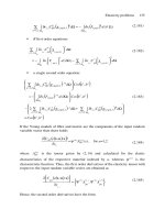
Consider now the equilibrium of an arbitrary finite part C of the body (see Fig. 2.1).
If we single this part out of the body, we should apply to it body forces q
v
and surface
tractions p
i
whose coordinate components p
x
, p
y
, and p
z
can be expressed, obviously,
by Eq. (2.2) in terms of stresses acting inside the volume C. Because the sum of the
s
z
s
y
n(l
x
, l
y
, l
z
)
p
s
(p
x
, p

y
, p
z
)
q
v
(q
x
, q
y
, q
z
)
t
yz
t
zx
t
xz
s
x
t
xy
t
yx
t
zy
dy
dz
dx

B
Fig. 2.3. Forces acting on an elementary tetrahedron.
34 Advanced mechanics of composite materials
components corresponding, for example, to the x-axis must be equal to zero, we have

v
q
x
dv +

s
p
x
ds = 0
where v and s are the volume and the surface area of the part of the body under
consideration. Substituting p
x
from Eq. (2.2) we get

s
(σ
x
l
x
+τ
yx
l
y
+τ
zx

l
z
)ds +

v
q
x
dv = 0 (x,y,z) (2.3)
Thus, we have three integral equilibrium equations, Eq. (2.3), which are valid for any
finite part of the body. To convert them into the corresponding differential equations, we
use Green’s integral transformation

s
(f
x
l
x
+f
y
l
y
+f
z
l
z
)ds =

v

∂f

x
∂x
+
∂f
y
∂y
+
∂f
z
∂z

dv (2.4)
which is valid for any three continuous, finite, and single-valued functions f(x, y,z) and
allows us to transform a surface integral into a volume one. Taking f
x
= σ
x
, f
y
= τ
yx
,
and f
z
= τ
zx
in Eq. (2.4) and using Eq. (2.3), we arrive at

v


∂σ
x
∂x
+
∂τ
yx
∂y
+
∂τ
zx
∂z
+q
x

dv = 0 (x,y,z)
Since these equations hold true for whatever the part of the solid may be, provided only
that it is within the solid, they yield
∂σ
x
∂x
+
∂τ
yx
∂y
+
∂τ
zx
∂z
+q
x

= 0 (x,y,z) (2.5)
Thus, we have arrived at three differential equilibrium equations that could also be derived
from the equilibrium conditions for the infinitesimal element shown in Fig. 2.2.
However, in order to keep part C of the body in Fig. 2.1 in equilibrium the sum of
the moments of all the forces applied to this part about any axis must be zero. By taking
moments about the z-axis we get the following integral equation

v
(q
x
y −q
y
x)dv +

s
(p
x
y −p
y
x)ds = 0
Using again Eqs. (2.2), (2.4), and taking into account Eq. (2.5) we finally arrive at the
symmetry conditions for shear stresses, i.e.,
τ
xy
= τ
yx
(x,y,z) (2.6)
Chapter 2. Fundamentals of mechanics of solids 35
So, we have three equilibrium equations, Eq. (2.5) which include six unknown stresses
σ

x
,σ
y
,σ
z
and τ
xy
,τ
xz
,τ
yz
.
Eq. (2.2) can be treated as force boundary conditions for the stressed state of a solid.
2.3. Stress transformation
Consider the transformation of a stress system from one Cartesian coordinate frame
to another. Suppose that the elementary tetrahedron shown in Fig. 2.3 is located inside
the body and that point B coincides with the origin 0 of Cartesian coordinates x, y,
and z in Fig. 2.1. Then, the oblique plane of the tetrahedron can be treated as a coor-
dinate plane z

= 0 of a new coordinate frame x

, y

, z

shown in Fig. 2.4 and such
that the normal element to the oblique plane coincides with the z

-axis, whereas axes

x

and y

are located in this plane. Component p
x
of the surface traction in Eq. (2.2)
can be treated now as the projection on the x-axis of stress σ acting on plane z

= 0.
Then, Eq. (2.2) can be presented in the following explicit form specifying projections of
stress σ
p
x
= σ
x
l
z

x
+τ
yx
l
z

y
+τ
zx
l
z


z
p
y
= σ
y
l
z

y
+τ
zy
l
z

z
+τ
xy
l
z

x
p
z
= σ
z
l
z

z

+τ
xz
l
z

x
+τ
yz
l
z

y
(2.7)
Y
Z
X
Y′(l
y
′
x
, l
y
′
y
, l
y
′
z
)
X′(l

x
′
x
, l
x
′
y
, l
x
′
z
)
Z′(l
z
′
x
, l
z
′
y
, l
z
′
z
)
s (p
x
, p
y
, p

z
)
t
z
′
y
′
t
z
′
x
′
s
z
′
Fig. 2.4. Rotation of the coordinate frame.
36 Advanced mechanics of composite materials
Here, l are directional cosines of axis z

with respect to axes x, y, and z (see Fig. 2.4 in
which the corresponding cosines of axes x

and y

are also presented). The normal stress
σ
z

can be found now as
σ

z

= p
x
l
z

x
+p
y
l
z

y
+p
z
l
z

z
= σ
x
l
2
z

x
+σ
y
l

2
z

y
+σ
z
l
2
z

z
+2τ
xy
l
z

x
l
z

y
+2τ
xz
l
z

x
l
z


z
+2τ
yz
l
z

y
l
z

z
(x

,y

,z

)
(2.8)
The final result was obtained with the aid of Eqs. (2.6) and (2.7). Changing x

for y

, y

for z

, and z

for x


, i.e., performing the appropriate permutation in Eq. (2.8) we can write
similar expressions for σ
x

and σ
y

.
The shear stress in the new coordinates is
τ
z

x

= p
x
l
x

x
+p
y
l
x

y
+p
z
l

x

z
= σ
x
l
x

x
l
z

x
+σ
y
l
x

y
l
z

y
+σ
z
l
x

z
l

z

z
+τ
xy
(l
x

x
l
z

y
+l
x

y
l
z

x
)
+τ
xz
(l
x

x
l
z


z
+l
x

z
l
z

x
) +τ
yz
(l
x

y
l
z

z
+l
x

x
l
z

y
)(x


,y

,z

) (2.9)
Permutation yields expressions for τ
x

y

and τ
y

z

.
2.4. Principal stresses
The foregoing equations, Eqs. (2.8) and (2.9), demonstrate stress transformations under
rotation of a coordinate frame. There exists a special position of this frame in which the
shear stresses acting on the coordinate planes vanish. Such coordinate axes are called the
principal axes, and the normal stresses that act on the corresponding coordinate planes
are referred to as the principal stresses.
To determine the principal stresses, assume that coordinates x

,y

, and z

, in Fig. 2.4 are
the principal coordinates. Then, according to the aforementioned property of the principal

coordinates, we should take τ
z

x

= τ
z

y

= 0 and σ
z

= σ for the plane z

= 0. This means
that p
x
= σl
z

x
,p
y
= σl
z

y
, and p
z

= σl
z

z
in Eqs. (2.7). Introducing new notations for
directional cosines of the principal axis, i.e., taking l
z

x
= l
px
,l
z

y
= l
py
,l
z

z
= l
pz
we
have from Eqs. (2.7)
(σ
x
−σ)l
px
+τ

xy
l
py
+τ
xz
l
pz
= 0
τ
xy
l
px
+(σ
y
−σ)l
py
+τ
yz
l
pz
= 0
τ
xz
l
px
+τ
yz
l
py
+(σ

z
−σ)l
pz
= 0
(2.10)
These equations were transformed with the aid of symmetry conditions for shear stresses,
Eq. (2.6). For some specified point of the body in the vicinity of which the principal
stresses are determined in terms of stresses referred to some fixed coordinate frame x, y, z
Chapter 2. Fundamentals of mechanics of solids 37
and known, Eqs. (2.10) comprise a homogeneous system of linear algebraic equations.
Formally, this system always has the trivial solution, i.e., l
px
= l
py
= l
pz
= 0 which we
can ignore because directional cosines should satisfy an evident condition following from
Eqs. (2.1), i.e.,
l
2
px
+l
2
py
+l
2
pz
= 1 (2.11)
So, we need to find a nonzero solution of Eqs. (2.10) which can exist if the determinant

of the set is zero. This condition yields the following cubic equation for σ
σ
3
−I
1
σ
2
−I
2
σ − I
3
= 0 (2.12)
in which
I
1
= σ
x
+σ
y
+σ
z
I
2
=−σ
x
σ
y
−σ
x
σ

z
−σ
y
σ
z
+τ
2
xy
+τ
2
xz
+τ
2
yz
I
3
= σ
x
σ
y
σ
z
+2τ
xy
τ
xz
τ
yz
−σ
x

τ
2
yz
−σ
y
τ
2
xz
−σ
z
τ
2
xy
(2.13)
are invariant characteristics (invariants) of the stressed state. This means that if we refer
the body to any Cartesian coordinate frame with directional cosines specified by Eqs. (2.1),
take the origin of this frame at some arbitrary point and change stresses in Eqs. (2.13)
with the aid of Eqs. (2.8) and (2.9), the values of I
1
,I
2
,I
3
at this point will be the same
for all such coordinate frames. Eq. (2.12) has three real roots that specify three principal
stresses σ
1
,σ
2
, and σ

3
. There is a convention according to which σ
1
≥ σ
2
≥ σ
3
, i.e.,
σ
1
is the maximum principal stress and σ
3
is the minimum one. If, for example, the
roots of Eq. (2.12) are 100 MPa, −200 MPa, and 0, then σ
1
= 100 MPa,σ
2
= 0, and
σ
3
=−200 MPa.
To demonstrate the procedure, consider a particular state of stress relevant to several
applications, namely, pure shear in the xy-plane. Let a thin square plate referred to coordi-
nates x, y, z be loaded with shear stresses τ uniformly distributed over the plate thickness
and along the edges (see Fig. 2.5).
One principal plane is evident – it is plane z = 0, which is free of shear stresses. To find
the other two planes, we should take in Eqs. (2.13) σ
x
= σ
y

= σ
z
= 0,τ
xz
= τ
yz
= 0,
and τ
xy
= τ. Then, Eq. (2.12) takes the form
σ
3
−τ
2
σ = 0
The first root of this equation gives σ = 0 and corresponds to plane z = 0. The other two
roots are σ =±τ . Thus, we have three principal stresses, i.e., σ
1
= τ, σ
2
= 0,σ
3
=−τ.
To find the planes corresponding to σ
1
and σ
3
we should put l
pz
= 0, substitute σ =±τ

into Eqs. (2.10), write them for the state of stress under study, and supplement this set
with Eq. (2.11). The final equations allowing us to find l
px
and l
py
are
±τl
px
+τl
py
= 0,l
2
px
+l
2
py
= 1
38 Advanced mechanics of composite materials
Y
t
t
t
s
1
s
3
x
1
x
3

x
2
t
45°
45°
Z
X
Fig. 2.5. Principal stresses under pure shear.
Solution of these equations yields l
px
=±1/
√
2 and l
py
=±1/
√
2, and means that
principal planes (or principal axes) make 45
◦
angles with axes x and y. Principal stresses
and principal coordinates x
1
, x
2
, and x
3
are shown in Fig. 2.5.
2.5. Displacements and strains
For any point of a solid (e.g., L or M in Fig. 2.1) coordinate component displacements
u

x
,u
y
, and u
z
can be introduced which specify the point displacements in the directions
of coordinate axes.
Consider an arbitrary infinitely small element LM characterized with its directional
cosines
l
x
=
dx
ds
,l
y
=
dy
ds
,l
z
=
dz
ds
(2.14)
The positions of this element before and after deformation are shown in Fig. 2.6. Suppose
that the displacements of the point L are u
x
,u
y

, and u
z
. Then, the displacements of the
point M should be
u
(1)
x
= u
x
+du
x
,u
(1)
y
= u
y
+du
y
,u
(1)
z
= u
z
+du
z
(2.15)
Since u
x
, u
y

, and u
z
are continuous functions of x, y, z,weget
du
x
=
∂u
x
∂x
dx +
∂u
y
∂y
dy +
∂u
z
∂z
dz (x,y, z) (2.16)
Chapter 2. Fundamentals of mechanics of solids 39
Y
dx
dx
1
M
1
N
1
L
1
ds′

1
ds
1
X
u
x
u
x
(1)
Z
L
ds′
ds
N
M
90°
a
Fig. 2.6. Displacement of an infinitesimal linear element.
It follows from Fig. 2.6 and Eqs. (2.15) and (2.16) that,
dx
1
= dx +u
(1)
x
−u
x
= dx +du
x
=


1 +
∂u
x
∂x

dx +
∂u
x
∂y
dy +
∂u
x
∂z
dz (x,y,z)
(2.17)
Introduce the strain of element LM as
ε =
ds
1
−ds
ds
(2.18)
After some rearrangements we arrive at
ε +
1
2
ε
2
=
1

2


ds
1
ds

2
−1

where
ds
2
1
= (dx
1
)
2
+(dy
1
)
2
+(dz
1
)
2
Substituting for dx
1
,dy
1

,dz
1
in their expressions from Eq. (2.17) and taking into account
Eqs. (2.14), we finally get
ε +
1
2
ε
2
= ε
xx
l
2
x
+ε
yy
l
2
y
+ε
zz
l
2
z
+ε
xy
l
x
l
y

+ε
xz
l
x
l
z
+ε
yz
l
y
l
z
(2.19)
40 Advanced mechanics of composite materials
where
ε
xx
=
∂u
x
∂x
+
1
2


∂u
x
∂x


2
+

∂u
y
∂x

2
+

∂u
z
∂x

2

(x,y,z)
ε
xy
=
∂u
x
∂y
+
∂u
y
∂x
+
∂u
x

∂x
∂u
x
∂y
+
∂u
y
∂x
∂u
y
∂y
+
∂u
z
∂x
∂u
z
∂y
(x,y,z)
(2.20)
Assuming that the strain is small, we can neglect the second term in the left-hand side of
Eq. (2.19). Moreover, we further suppose that the displacements are continuous functions
that change rather slowly with the change of coordinates. This allows us to neglect the
products of derivatives in Eqs. (2.20). As a result, we arrive at the following equation
ε = ε
x
l
2
x
+ε

y
l
2
y
+ε
z
l
2
z
+γ
xy
l
x
l
y
+γ
xz
l
x
l
z
+γ
yz
l
y
l
z
(2.21)
in which
ε

x
=
∂u
x
∂x
,ε
y
=
∂u
y
∂y
,ε
z
=
∂u
z
∂z
γ
xy
=
∂u
x
∂y
+
∂u
y
∂x
,γ
xz
=

∂u
x
∂z
+
∂u
z
∂x
,γ
yz
=
∂u
y
∂z
+
∂u
z
∂y
(2.22)
can be treated as linear strain–displacement equations. Taking l
x
= 1,l
y
= l
z
= 0in
Eqs. (2.22), i.e., directing element LM in Fig. 2.6 along the x-axis we can readily see
that ε
x
is the strain along the same x-axis. Similar reasoning shows that ε
y

and ε
z
in
Eqs. (2.22) are strains in the directions of axes y and z. To find out the physical meaning
of strains γ in Eqs. (2.22), consider two orthogonal line elements LM and LN and find
angle α that they make with each other after deformation (see Fig. 2.6), i.e.,
cos α =
dx
1
dx

1
+dy
1
dy

1
+dz
1
dz

1
ds
1
ds

1
(2.23)
Here, dx
1

,dy
1
, and dz
1
are specified with Eq. (2.17), ds
1
can be found from Eq. (2.18), and
dx

1
=

1 +
∂u
x
∂x

dx

+
∂u
x
∂y
dy

+
∂u
x
∂z
dz


(x,y,z)
ds

1
= ds

(1 +ε

)
(2.24)
Introduce directional cosines of element LN as
l

x
=
dx

ds

,l

y
=
dy

ds

,l


z
=
dz

ds

(2.25)
Chapter 2. Fundamentals of mechanics of solids 41
Since elements LM and LN are orthogonal, we have
l
x
l

x
+l
y
l

y
+l
z
l

z
= 0
Using Eqs. (2.14), (2.18), (2.24)–(2.26) and introducing the shear strain γ as the difference
between angles M
1
L
1

N
1
and MLN, i.e., as
γ =
π
2
−α
we can write Eq. (2.23) in the following form
sin γ =
1
(1 +ε)(1 +ε

)

2(ε
xx
l
x
l

x
+ε
yy
l
y
l

y
+ε
zz

l
z
l

z
) +ε
xy
(l
x
l

y
+l

x
l
y
)
+ε
xz
(l
x
l

z
+l

x
l
z

) + ε
yz
(l
y
l

z
+l

y
l
z
)

(2.26)
Linear approximation of Eq. (2.26) similar to Eq. (2.21) yields
γ = 2(ε
x
l
x
l

x
+ε
y
l
y
l

y

+ε
z
l
z
l

z
) +γ
xy
(l
x
l

y
+l

x
l
y
) +γ
xz
(l
x
l

z
+l

x
l

z
)
+γ
yz
(l
y
l

z
+l

y
l
z
) (2.27)
Here, ε
x
,ε
y
,ε
z
and γ
xy
,γ
xz
,γ
yz
components are determined with Eqs. (2.22). If we
now direct element LM along the x-axis and element LN along the y-axis putting
l

x
= 1,l
y
= l
z
= 0 and l

y
= 1,l

x
= l

z
= 0, Eq. (2.27) yields γ = γ
xy
. Thus,
γ
xy
,γ
xz
, and γ
yz
are shear strains that are equal to the changes of angles between axes
x and y, x and z, y and z, respectively.
2.6. Transformation of small strains
Consider small strains in Eqs. (2.22) and study their transformation under rotation of
the coordinate frame. Suppose that x

,y


,z

in Fig. 2.4 form a new coordinate frame
rotated with respect to original frame x, y, z. Since Eqs. (2.22) are valid for any Cartesian
coordinate frame, we have
ε
x

=
∂u
x

∂x

,γ
x

y

=
∂u
x

∂y

+
∂u
y


∂x

(x,y,z) (2.28)
Here, u
x

,u
y

, and u
z

are displacements along the axes x

,y

,z

which can be related to
displacements u
x
,u
y
, and u
z
of the same point by the following linear equations
u
x

= u

x
l
x

x
+u
y
l
x

y
+u
z
l
x

z
(x,y,z) (2.29)
42 Advanced mechanics of composite materials
Similar relations can be written for the derivatives of displacement with respect to variables
x

,y

,z

and x, y, z, i.e.,
∂u
∂x


=
∂u
∂x
l
x

x
+
∂u
∂y
l
x

y
+
∂u
∂z
l
x

z
(x,y,z) (2.30)
Substituting displacements, Eq. (2.29), into Eqs. (2.28), and transforming to variables x,
y, z with the aid of Eqs. (2.30), and taking into account Eqs. (2.22), we arrive at
ε
x

= ε
x
l

2
x

x
+ε
y
l
2
x

y
+ε
z
l
2
x

z
+γ
xy
l
x

x
l
x

y
+γ
xz

l
x

x
l
x

z
+γ
yz
l
x

y
l
x

z
(x,y,z)
γ
x

y

= 2ε
x
l
x

x

l
y

x
+2ε
y
l
x

y
l
y

y
+2ε
z
l
x

z
l
y

z
+γ
xy
(l
x

x

l
y

y
+l
x

y
l
y

x
) (2.31)
+γ
xz
(l
x

x
l
y

z
+l
x

z
l
y


x
) +γ
yz
(l
x

y
l
y

z
+l
x

z
l
y

y
) (x,y, z)
These strain transformations are similar to the stress transformations determined by
Eqs. (2.8) and (2.9).
2.7. Compatibility equations
Consider strain–displacement equations, Eqs. (2.22), and try to determine displacements
u
x
, u
y
, and u
z

in terms of strains ε
x
, ε
y
, ε
z
and γ
xy
, γ
xz
γ
yz
. As can be seen, there are six
equations containing only three unknown displacements. In the general case, such a set
of equations is not consistent, and some compatibility conditions should be imposed on
the strains to provide the existence of a solution. To derive these conditions, decompose
derivatives of the displacements as follows
∂u
x
∂x
= ε
x
,
∂u
x
∂y
=
1
2
γ

xy
−ω
z
,
∂u
x
∂z
=
1
2
γ
xz
+ω
y
(x,y,z) (2.32)
Here
ω
z
=
1
2

∂u
y
∂x
−
∂u
x
∂y


(x,y,z) (2.33)
is the angle of rotation of a body element (such as the cubic element shown in Fig. 2.1)
around the z-axis. Three Eqs. (2.32) including one and the same displacement u
x
allow
us to construct three couples of mixed second-order derivatives of u
x
with respect to x
and y or y and x, x and z or z and x, y and z or z and y. As long as the sequence
of differentiation does not influence the result and since there are two other groups of
Chapter 2. Fundamentals of mechanics of solids 43
equations in Eqs. (2.32), we arrive at nine compatibility conditions that can be presented as
∂ω
x
∂x
=
1
2

∂γ
xz
∂y
−
∂γ
xy
∂z

(x,y,z)
∂ω
x

∂y
=
1
2
∂γ
yz
∂y
−
∂ε
y
∂z
(x,y,z),
∂ω
x
∂z
=−
1
2
∂γ
yz
∂z
+
∂ε
z
∂y
(x,y,z)
(2.34)
These equations are similar to Eqs. (2.32), i.e., they allow us to determine rotation angles
only if some compatibility conditions are valid. These conditions compose the set of
compatibility equations for strains and have the following final form

k
xy
(ε, γ ) = 0,r
x
(ε, γ ) = 0 (x,y,z) (2.35)
where
k
xy
(ε, γ ) =
∂
2
ε
x
∂y
2
+
∂
2
ε
y
∂x
2
−
∂
2
γ
xy
∂x∂y
(x,y,z)
r

x
(ε, γ ) =
∂
2
ε
x
∂y∂z
−
1
2
∂
∂x

∂γ
xy
∂z
+
∂γ
xz
∂y
−
∂γ
yz
∂x

(x,y,z)
(2.36)
If strains ε
x
,ε

y
,ε
z
and γ
xy
,γ
xz
,γ
yz
satisfy Eqs. (2.35), we can find rotation angles
ω
x
,ω
y
,ω
z
integrating Eqs. (2.34) and then determine displacements u
x
,u
y
,u
z
integrating
Eqs. (2.32).
The six compatibility equations, Eqs. (2.35), derived formally as compatibility condi-
tions for Eqs. (2.32), have a simple physical meaning. Suppose that we have a continuous
solid as shown in Fig. 2.1 and divide it into a set of pieces that perfectly match each
other. Now, apply some strains to each of these pieces. Obviously, for arbitrary strains,
the deformed pieces cannot be assembled into a continuous deformed solid. This will
happen only under the condition that the strains satisfy Eqs. (2.35). However, even if the

strains do not satisfy Eqs. (2.35), we can assume that the solid is continuous but in a more
general Riemannian (curved) space rather than in traditional Euclidean space in which the
solid existed before the deformation (Vasiliev and Gurdal, 1999). Then, six quantities k
and r in Eqs. (2.36), being nonzero, specify curvatures of the Riemannian space caused by
small strains ε and γ . The compatibility equations, Eqs. (2.35), require these curvatures
to be equal to zero which means that the solid should remain in the Euclidean space under
deformation.
2.8. Admissible static and kinematic fields
In solid mechanics, we introduce static field variables which are stresses and kinematic
field variables which are displacements and strains.
44 Advanced mechanics of composite materials
The static field is said to be statically admissible if the stresses satisfy equilibrium
equations, Eq. (2.5), and are in equilibrium with surface tractions on the body surface S
σ
where these tractions are given (see Fig. 2.1), i.e., if Eq. (2.2) are satisfied on S
σ
.
The kinematic field is referred to as kinematically admissible if displacements and
strains are linked by strain–displacement equations, Eqs. (2.22), and displacements satisfy
kinematic boundary conditions on the surface S
u
where displacements are prescribed (see
Fig. 2.1).
Actual stresses and displacements belong, naturally, to the corresponding admissi-
ble fields though actual stresses must in addition provide admissible displacements,
whereas actual displacements should be associated with admissible stresses. Mutual cor-
respondence between static and kinematic variables is established through the so-called
constitutive equations that are considered in the next section.
2.9. Constitutive equations for an elastic solid
Consider a solid loaded with body and surface forces as in Fig. 2.1. These forces

induce some stresses, displacements, and strains that compose the fields of actual static
and kinematic variables. Introduce some infinitesimal additional displacements du
x
,du
y
,
and du
z
such that they belong to a kinematically admissible field. This means that there
exist equations that are similar to Eqs. (2.22), i.e.,
dε
x
=
∂
∂x
(du
x
), dγ
xy
=
∂
∂y
(du
x
) +
∂
∂x
(du
y
) (x,y, z) (2.37)

and specify additional strains.
Since additional displacements are infinitely small, we can assume that external forces
do not change under such variation of the displacements (here we do not consider special
cases in which external forces depend on displacements of the points at which these forces
are applied). Then we can calculate the work performed by the forces by multiplying forces
by the corresponding increments of the displacements and writing the total work of body
forces and surface tractions as
dW =

V
(q
x
du
x
+q
y
du
y
+q
z
du
z
)dV +

S
(p
x
du
x
+p

y
du
y
+p
z
du
z
)dS
(2.38)
Here, V and S are the body volume and external surface of the body in Fig. 2.1. Actu-
ally, we must write the surface integral in Eq. (2.38) only for the surface S
σ
on which
the forces are given. However, since the increments of the displacements belong to a
kinematically admissible field, they are equal to zero on S
u
, and the integral can be
written for the whole surface of the body. To proceed, we express p
x
, p
y
, and p
z
in
terms of stresses with the aid of Eq. (2.2) and transform the surface integral into a
Chapter 2. Fundamentals of mechanics of solids 45
volume one using Eq. (2.4). For the sake of brevity, consider only x-components of
forces and displacement in Eq. (2.38). We have in several steps

V

q
x
du
x
+

S
p
x
du
x
ds =

V
q
x
du
x
+

S
(σ
x
l
x
+τ
yx
l
y
+τ

zx
l
z
)du
x
dS
=

V

q
x
du
x
+
∂
∂x
(σ
x
du
x
) +
∂
∂y
(τ
yx
du
x
) +
∂

∂z
(τ
zx
du
x
)

dV
=

V

q
x
+
∂σ
x
∂x
+
∂τ
yx
∂y
+
∂τ
zx
∂z

du
x
+σ

x
∂
∂x
(du
x
)
+τ
yx
∂
∂y
(du
x
) +τ
zx
∂
∂z
(du
x
)

dV
=

V

σ
x
dε
x
+τ

xy
∂
∂y
(du
x
) +τ
xz
∂
∂z
(du
x
)

dV
The last transformation step has been performed with due regard to Eqs. (2.5), (2.6), and
(2.37). Finally, Eq. (2.38) takes the form
dW =

V
(σ
x
dε
x
+σ
y
dε
y
+σ
z
dε

z
+τ
xy
dγ
xy
+τ
xz
dγ
xz
+τ
yz
dγ
yz
)dV (2.39)
Since the right-hand side of this equation includes only internal variables, i.e., stresses
and strains, we can conclude that the foregoing formal rearrangement actually allows us
to transform the work of external forces into the work of internal forces or into potential
energy accumulated in the body. For further derivation, let us introduce for the sake
of brevity new notations for coordinates and use subscripts 1, 2, 3 instead of x, y, z,
respectively. We also use the following notations for stresses and strains
σ
x
= σ
11
,σ
y
= σ
22
,σ
z

= σ
33
τ
xy
= σ
12
= σ
21
,τ
xz
= σ
13
= σ
31
,τ
yz
= σ
23
= σ
32
ε
x
= ε
11
,ε
y
= ε
22
,ε
z

= ε
33
γ
xy
= 2ε
12
= 2ε
21
,γ
xz
= 2ε
13
= 2ε
31
,γ
yz
= 2ε
23
= 2ε
32
Then, Eq. (2.39) can be written as
dW =

V
dUdV (2.40)
46 Advanced mechanics of composite materials
where
dU = σ
ij
dε

ij
(2.41)
This form of equation implies summation over repeated subscripts i, j = 1, 2, 3.
It should be emphasized that by now dU is just a symbol, which does not mean that
there exists function U and that dU is its differential. This meaning for dU is correct only
if we restrict ourselves to the consideration of an elastic material described in Section 1.1.
For such a material, the difference between the body potential energy corresponding to
some initial state A and the energy corresponding to some other state B does not depend
on the way used to transform the body from state A to state B. In other words, the
integral

B
A
σ
ij
dε
ij
= U(B)− U(A)
does not depend on the path of integration. This means that the element of integration is
a complete differential of function U depending on ε
ij
, i.e., that
dU =
∂U
∂ε
ij
dε
ij
Comparing this result with Eq. (2.41) we arrive at Green’s formulas
σ

ij
=
∂U
∂ε
ij
(2.42)
that are valid for any elastic material. The function U(ε
ij
) can be referred to as specific
strain energy (energy accumulated in the unit of body volume) or elastic potential. The
potential U can be expanded into a Taylor series with respect to strains, i.e.,
U(ε
ij
) = s
0
+s
ij
ε
ij
+
1
2
s
ij kl
ε
ij
ε
kl
+··· (2.43)
where

s
0
= U(ε
ij
= 0), s
ij
=
∂U
∂ε
ij




ε
ij
=0
,s
ij kl
=
∂
2
U
∂ε
ij
∂ε
kl





ε
ij
=0,ε
kl
=0
(2.44)
Assume that for the initial state of the body, corresponding to zero external forces, we
have ε
ij
= 0,σ
ij
= 0,U= 0. Then, s
0
= 0 and s
ij
= 0 according to Eq. (2.42).