ADVANCED MECHANICS OF COMPOSITE MATERIALS Episode 5 potx

Chapter 3. Mechanics of a unidirectional ply 127
0
400
800
1200
0 0.2
0.4
0.8 1
s
1
, MPa
w
f
(2)
w
f
(2)
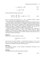
Fig. 3.71. Dependence of the longitudinal strength of unidirectional carbon–glass epoxy composite on the
volume fraction of glass fibers.
The threshold value of w
(2)
f
indicating the minimum amount of the second-type fibers
that is sufficient to withstand the load after the failure of the first-type fibers can be found
from the condition
ε
∗
1
= ε
(2)
f

(Skudra et al., 1989). The final result is as follows
w
(2)
f
=
E
(1)
f
v
f
ε
(1)
f
−(1 −v
f
)E
m

ε
(2)
f
−ε
(1)
f

v
f

E
(1)

f
ε
(1)
f
+E
(2)
f

ε
(2)
f
−ε
(1)
f

For w
(2)
f
< w
(2)
f
, material strength can be calculated as σ
1
= E
1
ε
(1)
f
whereas for w
(2)

f
>
w
(2)
f
, σ
1
= E
∗
1
ε
(2)
f
. The corresponding theoretical prediction of the dependence of material
strength on w
(2)
f
is shown in Fig. 3.71 (Skudra et al., 1989).
3.6. Composites with high fiber fraction
We now return to Fig. 3.44, which shows the dependence of the tensile longitudinal
strength of unidirectional composites on the fiber volume fraction v
f
. As follows from
this figure, the strength increases up to v
f
, which is close to 0.7 and becomes lower for
higher fiber volume fractions. This is a typical feature of unidirectional fibrous composites
(Andreevskaiya, 1966). However, there are some experimental results (e.g., Roginskii
and Egorov, 1966) showing that material strength can increase up to v
f

= 0.88, which
corresponds to the maximum theoretical fiber volume fraction discussed in Section 3.1.
The reason that the material strength usually starts to decrease at higher fiber volume
fractions is associated with material porosity, which becomes significant for materials
with a shortage of resin. By reducing the material porosity, we can increase material
tensile strength for high fiber volume fractions.
128 Advanced mechanics of composite materials
(a) (b)
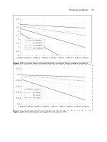
Fig. 3.72. Cross-section of aramid–epoxy composite with high fiber fraction: (a) initial structure; (b) structure
with delaminated fibers.
Moreover, applying the correct combination of compacting pressure and temperature to
composites with organic (aramid or polyethylene) fibers, we can deform the fiber cross-
sections and reach a value of v
f
that would be close to unity. Such composite materials
studied by Golovkin (1985), Kharchenko (1999), and other researchers are referred to as
composites with high fiber fraction (CHFF). The cross-section of a typical CHFF is shown
in Fig. 3.72.
Table 3.7
Properties of aramid–epoxy composites with high fiber fraction.
Property Fiber volume fraction, v
f
0.65 0.92 0.96
Density, ρ (g/cm
3
) 1.33 1.38 1.41
Longitudinal modulus, E
1
(GPa) 85 118 127
Transverse modulus, E

2
(GPa) 3.3 2.1 4.5
Shear modulus, G
12
(GPa) 1.6 1.7 —
Longitudinal tensile strength,
σ
+
1
(MPa) 2200 2800 2800
Longitudinal compressive strength,
σ
−
1
(MPa) 293 295 310
Transverse tensile strength,
σ
+
2
(MPa) 22 12 —
Transverse compressive strength,
σ
−
2
(MPa) 118 48 —
In-plane shear strength,
τ
12
(MPa) 41 28 18
Chapter 3. Mechanics of a unidirectional ply 129

The properties of aramid–epoxy CHFF are listed in Table 3.7 (Kharchenko, 1999).
Comparing traditional composites (v
f
= 0.65) with CHFF, we can conclude that CHFF
have significantly higher longitudinal modulus (up to 50%) and longitudinal tensile
strength (up to 30%), whereas the density is only 6% higher. However, the transverse
and shear strengths of CHFF are lower than those of traditional composites. Because of
this, composites with high fiber fraction can be efficient in composite structures whose
loading induces high tensile stresses acting mainly along the fibers, e.g., in cables, pressure
vessels, etc.
3.7. Phenomenological homogeneous model of a ply
It follows from the foregoing discussion that micromechanical analysis provides very
approximate predictions for the ply stiffness and only qualitative information concerning
the ply strength. However, the design and analysis of composite structures require quite
accurate and reliable information about the properties of the ply as the basic element
of composite structures. This information is provided by experimental methods as dis-
cussed above. As a result, the ply is presented as an orthotropic homogeneous material
possessing some apparent (effective) mechanical characteristics determined experimen-
tally. This means that, on the ply level, we use a phenomenological model of a composite
material (see Section 1.1) that ignores its actual microstructure.
It should be emphasized that this model, being quite natural and realistic for the majority
of applications, sometimes does not allow us to predict actual material behavior. To demon-
strate this, consider a problem of biaxial compression of a unidirectional composite in the
23-plane as in Fig. 3.73. Testing a glass–epoxy composite material described by Koltunov
et al. (1977) shows a surprising result – its strength is about
σ = 1200 MPa, which is
quite close to the level of material strength under longitudinal tension, and material failure
is accompanied by fiber breakage typical for longitudinal tension.
The phenomenological model fails to predict this mode of failure. Indeed, the average
stress in the longitudinal direction specified by Eq. (3.75) is equal to zero under loading

shown in Fig. 3.73, i.e.,
σ
1
= σ
f
1
v
f
+σ
m
1
v
m
= 0 (3.127)
To apply the first-order micromechanical model considered in Section 3.3, we generalize
constitutive equations, Eqs. (3.63), for the three-dimensional stress state of the fibers and
the matrix as
ε
f,m
1
=
1
E
f,m

σ
f,m
1
−ν
f,m


σ
f,m
2
+σ
f,m
3

(1, 2, 3) (3.128)
Changing 1 for 2, 2 for 3, and 3 for 1, we can write the corresponding equations for ε
2
and ε
3
.
130 Advanced mechanics of composite materials
Suppose that the stresses acting in the fibers and in the matrix in the plane of loading
are the same, i.e.,
σ
f
2
= σ
f
3
= σ
m
2
= σ
m
3
=−σ (3.129)

and that ε
f
1
= ε
m
1
. Substituting ε
f
1
and ε
m
1
from Eqs. (3.128), we get with due regard to
Eqs. (3.129)
1
E
f

σ
f
1
+2ν
f
σ

=
1
E
m


σ
m
1
+2ν
m
σ

In conjunction with Eq. (3.127), this equation allows us to find σ
f
1
, which has the form
σ
f
1
=
2σ(E
f
ν
m
−E
m
ν
f
)v
m
E
f
v
f
+E

m
v
m
Simplifying this result for the situation E
f
 E
m
, we arrive at
σ
f
1
= 2σ
ν
m
v
m
v
f
Thus, the loading shown in Fig. 3.73 indeed induces tension in the fibers as can be revealed
using the micromechanical model. The ultimate stress can be expressed in terms of the
fibers’ strength
σ
f
as
σ =
1
2
σ
f
v

f
ν
m
v
m
1
s
s
s
s
3
2
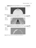
Fig. 3.73. Biaxial compression of a unidirectional composite.
Chapter 3. Mechanics of a unidirectional ply 131
The actual material strength is not as high as follows from this equation, which is
derived under the condition that the adhesive strength between the fibers and the matrix is
infinitely high. Tension of fibers is induced by the matrix that expands in the 1-direction
(see Fig. 3.73) due to Poisson’s effect and interacts with fibers through shear stresses
whose maximum value is limited by the fiber–matrix adhesion strength. Under high shear
stress, debonding of the fibers can occur, reducing the material strength, which is, nev-
ertheless, very high. This effect is utilized in composite shells with radial reinforcement
designed to withstand an external pressure of high intensity (Koltunov et al., 1977).
3.8. References
Abu-Farsakh, G.A., Abdel-Jawad, Y.A. and Abu-Laila, Kh.M. (2000). Micromechanical characterization of
tensile strength of fiber composite materials. Mechanics of Composite Materials Structures, 7(1), 105–122.
Andreevskaya, G.D. (1966). High-strength Oriented Fiberglass Plastics. Nauka, Moscow (in Russian).
Bogdanovich, A.E. and Pastore, C.M. (1996). Mechanics of Textile and Laminated Composites. Chapman &
Hall, London.
Chiao, T.T. (1979). Some interesting mechanical behaviors of fiber composite materials. In Proc. of 1st USA-
USSR Symposium on Fracture of Composite Materials, Riga, USSR, 4–7 September, 1978 (G.C. Sih and

V.P. Tamuzh eds.). Sijthoff and Noordhoff, Alphen aan den Rijn., pp. 385–392.
Crasto, A.S. and Kim, R.Y. (1993). An improved test specimen to determine composite compression strength.
In Proc. 9th Int. Conf. on Composite Materials (ICCM/9), Madrid, 12–16 July 1993, Vol. 6, Composite
Properties and Applications. Woodhead Publishing Ltd., pp. 621–630.
Fukuda, H., Miyazawa, T. and Tomatsu, H. (1993). Strength distribution of monofilaments used for advanced
composites. In Proc. 9th Int. Conf. on Composite Materials (ICCM/9), Madrid, 12–16 July 1993, Vol. 6,
Composite Properties and Applications. Woodhead Publishing Ltd., pp. 687–694.
Gilman, J.J. (1959). Cleavage, Ductility and Tenacity in Crystals. In Fracture. Wiley, New York.
Golovkin, G.S. (1985). Manufacturing parameters of the formation process for ultimately reinforced organic
plastics. Plastics, 4, 31–33 (in Russian).
Goodey, W.J. (1946). Stress diffusion problems. Aircraft Eng. June 1946, 195–198; July 1946, 227–234; August
1946, 271–276; September 1946, 313–316; October 1946, 343–346; November 1946, 385–389.
Griffith, A.A. (1920). The phenomenon of rupture and flow in solids. Philosophical Transactions of the Royal
Society,A221, 147–166.
Gunyaev, G.M. (1981). Structure and Properties of Polymeric Fibrous Composites. Khimia, Moscow
(in Russian).
Hashin, Z. and Rosen, B.W. (1964). The elastic moduli of fiber reinforced materials. Journal of Applied
Mechanics, 31E, 223–232.
Jones, R.M. (1999). Mechanics of Composite Materials, 2nd edn. Taylor & Francis, Philadelphia, PA.
Kharchenko, E.F. (1999). High-strength Ultimately Reinforced Organic Plastics. Moscow (in Russian).
Koltunov, M.A., Pleshkov, L.V., Kanovich, M.Z., Roginskii, S.L. and Natrusov, V.I. (1977). High-strength
glass-reinforced plastic shells with radial orientation of the reinforcement. Polymer Mechanics/Mechanics of
Composite Materials, 13(6), 928–930.
Kondo, K. and Aoki, T. (1982). Longitudinal shear modulus of unidirectional composites. In Proc. 4th Int. Conf.
on Composite Materials (ICCM-IV), Vol. 1, Progr. in Sci. and Eng. of Composites (Hayashi, Kawata and
Umeka eds.). Tokyo, 1982, pp. 357–364.
Lagace, P.A. (1985). Nonlinear stress–strain behavior of graphite/epoxy laminates. AIAA Journal, 223(10),
1583–1589.
Lee, D.J., Jeong, T.H. and Kim, H.G. (1995). Effective longitudinal shear modulus of unidirectional composites.
In Proc. 10th Int. Conf. on Composite Materials (ICCM-10), Vol. 4, Characterization and Ceramic Matrix

Composites
, Canada, 1995, pp. 171–178.
132 Advanced mechanics of composite materials
Mikelsons, M.Ya. and Gutans, Yu.A. (1984). Failure of the aluminum–boron plastic in static and cyclic tensile
loading. Mechanics of Composite Materials, 20(1), 44–52.
Mileiko, S.T. (1982). Mechanics of metal-matrix fibrous composites. In Mechanics of Composites (Obraztsov, I.F.
and Vasiliev, V.V. eds.). Mir, Moscow, pp. 129–165.
Peters, S.T. (1998). Handbook of Composites. 2nd edn. (S.T. Peters ed.). Chapman & Hall, London.
Roginskii, S.L. and Egorov, N.G. (1966). Effect of prestress on the strength of metal shells reinforced with a
glass-reinforced plastic. Polymer Mechanics/Mechanics of Composite Materials, 2(2), 176–178.
Skudra, A.M., Bulavs, F.Ya., Gurvich, M.R. and Kruklinsh, A.A. (1989). Elements of Structural Mechanics of
Composite Truss Systems. Riga, Zinatne, (in Russian).
Tarnopol’skii, Yu.M. and Roze, A.V. (1969). Specific Features of Analysis for Structural Elements of Reinforced
Plastics, Riga, Zinatne, (in Russian).
Tarnopol’skii, Yu.M. and Kincis, T.Ya. (1985). Static Test Methods for Composites. Van Nostrand Reinhold,
New York.
Tikhomirov, P.V. and Yushanov, S.P. (1980). Stress distribution after the fracture of fibers in a unidirectional
composite. In Mechanics of Composite Materials, Riga, pp. 28–43 (in Russian).
Timoshenko, S.P. and Gere, J.M. (1961). Theory of Elastic Stability, 2nd edn. McGraw-Hill, New York.
Van Fo Fy (Vanin), G.A. (1966). Elastic constants and state of stress of glass-reinforced strip. Journal of Polymer
Mechanics, 2(4), 368–372.
Vasiliev, V.V. and Tarnopol’skii, Yu.M. (1990). Composite Materials. Handbook (V.V. Vasiliev, and
Yu.M. Tarnopol’skii eds.). Mashinostroenie, Moscow, (in Russian).
Woolstencroft, D.H., Haresceugh, R.I. and Curtis, A.R. (1982). The compressive behavior of carbon fiber
reinforced plastic. In Proc. 4th Int. Conf. on Composite Materials (ICCM-IV), Vol. 1, Progr. in Sci. and Eng.
of Composites (Hayashi, Kawata and Umeka eds.). Tokyo, 1982, pp. 439–446.
Zabolotskii, A.A. and Varshavskii, V.Ya. (1984). Multireinforced (Hybrid) composite materials. In Science and
Technology Reviews, Composite Materials, Part 2, Moscow.
Chapter 4
MECHANICS OF A COMPOSITE LAYER

A typical composite laminate consists of individual layers (see Fig. 4.1) which are
usually made of unidirectional plies with the same or regularly alternating orientation.
A layer can also be made from metal, thermosetting or thermoplastic polymer, or fabric
or can have a spatial three-dimensionally reinforced structure. In contrast to a ply as
considered in Chapter 3, a layer is generally referred to the global coordinate frame x, y,
and z of the structural element rather than to coordinates 1, 2, and 3 associated with the
ply orientation. Usually, a layer is much thicker than a ply and has a more complicated
structure, but this structure does not change through its thickness, or this change is ignored.
Thus, a layer can be defined as a three-dimensional structural element that is uniform in
the transverse (normal to the layer plane) direction.
4.1. Isotropic layer
The simplest layer that can be observed in composite laminates is an isotropic layer of
metal or thermoplastic polymer that is used to protect the composite material (Fig. 4.2)
and to provide tightness. For example, filament-wound composite pressure vessels usually
have a sealing metal (Fig. 4.3) or thermoplastic (Fig. 4.4) internal liner, which can also be
used as a mandrel for winding. Since the layer is isotropic, we need only one coordinate
system and let it be the global coordinate frame as in Fig. 4.5.
4.1.1. Linear elastic model
The explicit form of Hooke’s law in Eqs. (2.48) and (2.54) can be written as
ε
x
=
1
E
(σ
x
−νσ
y
−νσ
z

), γ
xy
=
τ
xy
G
ε
y
=
1
E
(σ
y
−νσ
x
−νσ
z
), γ
xz
=
τ
xz
G
ε
z
=
1
E
(σ
z

−νσ
x
−νσ
y
), γ
yz
=
τ
yz
G
(4.1)
133
Fig. 4.1. Laminated structure of a composite pipe.
Fig. 4.2. Composite drive shaft with external metal protection layer. Courtesy of CRISM.
Chapter 4. Mechanics of a composite layer 135
Fig. 4.3. Aluminum liner for a composite pressure vessel.
Fig. 4.4. Filament-wound composite pressure vessel with a polyethylene liner. Courtesy of CRISM.
136 Advanced mechanics of composite materials
s
z
s
x
s
y
t
yz
t
yz
t
xy

t
xy
t
xz
t
xz
x
y
z
Fig. 4.5. An isotropic layer.
where E is the modulus of elasticity, ν the Poisson’s ratio, and G is the shear modulus
which can be expressed in terms of E and ν with Eq. (2.57). Adding Eqs. (4.1) for normal
strains we get
ε
0
=
1
K
σ
0
(4.2)
where
ε
0
= ε
x
+ε
y
+ε
z

(4.3)
is the volume deformation. For small strains, the volume dV
1
of an infinitesimal material
element after deformation can be found knowing the volume dV before the deformation
and ε
0
as
dV
1
= (1 + ε
0
)dV
Volume deformation is related to the mean stress
σ
0
=
1
3
(σ
x
+σ
y
+σ
z
) (4.4)
through the volume or bulk modulus
K =
E
3(1 −2ν)

(4.5)
For ν = 1/2, K →∞, ε
0
= 0, and dV
1
= dV for any stress. Such materials are called
incompressible – they do not change their volume under deformation and can change only
their shape.
Chapter 4. Mechanics of a composite layer 137
The foregoing equations correspond to the general three-dimensional stress state of a
layer. However, working as a structural element of a thin-walled composite laminate, a
layer is usually loaded with a system of stresses one of which, namely, transverse normal
stress σ
z
is much less than the other stresses. Bearing this in mind, we can neglect the
terms in Eqs. (4.1) that include σ
z
and write these equations in a simplified form
ε
x
=
1
E
(σ
x
−νσ
y
), ε
y
=

1
E
(σ
y
−νσ
x
)
γ
xy
=
τ
xy
G
,γ
xz
=
τ
xz
G
,γ
yz
=
τ
yz
G
(4.6)
or
σ
x
= E(ε

x
+νε
y
), σ
y
= E(ε
y
+νε
x
)
τ
xy
= Gγ
xy
,τ
xz
= Gγ
xz
,τ
yz
= Gγ
yz
(4.7)
where
E = E/(1 −ν
2
).
4.1.2. Nonlinear models
Materials of metal and polymeric layers considered in this section demonstrate linear
response only under moderate stresses (see Figs. 1.11 and 1.14). Further loading results

in nonlinear behavior, to describe which we need to apply one of the nonlinear material
models discussed in Section 1.1.
A relatively simple nonlinear constitutive theory suitable for polymeric layers can be
constructed using a nonlinear elastic material model (see Fig. 1.2). In the strict sense,
this model can be applied to materials whose stress–strain curves are the same for active
loading and unloading. However, normally structural analysis is undertaken only for active
loading. If unloading is not considered, an elastic model can be formally used for materials
that are not perfectly elastic.
There exist a number of models developed to describe the nonlinear behavior of highly
deformable elastomers such as rubber (Green and Adkins, 1960). Polymeric materials
used to form isotropic layers of composite laminates admitting, in principal, high strains
usually do not demonstrate them in composite structures whose deformation is governed
by fibers with relatively low ultimate elongation (1–3%). So, creating the model, we can
restrict ourselves to the case of small strains, i.e., to materials whose typical stress–strain
diagram is shown in Fig. 4.6.
A natural way is to apply Eqs. (2.41) and (2.42), i.e., (we use tensor notations for
stresses and strains introduced in Section 2.9 and the rule of summation over repeated
subscripts)
dU = σ
ij
dε
ij
,σ
ij
=
∂
U
∂
ε
ij

(4.8)
138 Advanced mechanics of composite materials
0
0 0.5 1 1.5 2 2.5
10
20
30
40
50
s, MPa
e, %
Fig. 4.6. A typical stress–strain diagram (circles) for a polymeric film and its cubic approximation (solid line).
Approximation of elastic potential U as a function of ε
ij
with some unknown parameters
allows us to write constitutive equations directly using the second relation in Eqs. (4.8).
However, the polynomial approximation similar to Eq. (2.43), which is the most simple
and natural results in a constitutive equation of the type σ = Sε
n
, in which S is some
stiffness coefficient and n is an integer. As can be seen in Fig. 4.7, the resulting stress–
strain curve is not typical for the materials under study. Better agreement with nonlinear
experimental diagrams presented, e.g., in Fig. 4.6, is demonstrated by the curve specified
by the equation ε = Cσ
n
, in which C is some compliance coefficient. To arrive at this
form of a constitutive equation, we need to have a relationship similar to the second one in
Eqs. (4.8) but allowing us to express strains in terms of stresses. Such relationships exist
and are known as Castigliano’s formulas. To derive them, introduce the complementary
elastic potential U

c
in accordance with the following equation
dU
c
= ε
ij
dσ
ij
(4.9)
The term ‘complementary’ becomes clear if we consider a bar in Fig. 1.1 and the corre-
sponding stress–strain curve in Fig. 4.8. The area 0BC below the curve represents U in
accordance with the first equation in Eqs. (4.8), whereas the area 0AC above the curve is
equal to U
c
. As shown in Section 2.9, dU in Eqs. (4.8) is an exact differential. To prove
the same for dU
c
, consider the following sum
dU +dU
c
= σ
ij
dε
ij
+ε
ij
dσ
ij
= d(σ
ij

ε
ij
)
Chapter 4. Mechanics of a composite layer 139
s
s = Se
n
e = Cs
n
e
Fig. 4.7. Two forms of approximation of the stress–strain curve.
A
ds
s
s
0
B
U
c
U
dee
e
C
Fig. 4.8. Geometric interpretation of elastic potential, U, and complementary potential, U
c
.
140 Advanced mechanics of composite materials
which is obviously an exact differential. Since dU in this sum is also an exact differential,
dU
c

should have the same property and can be expressed as
dU
c
=
∂
U
c
∂
σ
ij
dσ
ij
Comparing this result with Eq. (4.9), we arrive at Castigliano’s formulae
ε
ij
=
∂
U
c
∂
σ
ij
(4.10)
which are valid for any elastic solid (for a linear elastic solid, U
c
= U).
The complementary potential, U
c
, in general, depends on stresses, but for an isotropic
material, Eq. (4.10) should yield invariant constitutive equations that do not depend on the

direction of coordinate axes. This means that U
c
should depend on stress invariants I
1
, I
2
,
and I
3
in Eqs. (2.13). Using different approximations for the function U
c
(I
1
, I
2
, I
3
), we
can construct different classes of nonlinear elastic models. Existing experimental verifi-
cation of such models shows that the dependence of U
c
on I
3
can be neglected. Thus, we
can present the complementary potential in a simplified form U
c
(I
1
, I
2

) and expand this
function as a Taylor series as
U
c
= c
0
+c
11
I
1
+
1
2
c
12
I
2
1
+
1
3!
c
13
I
3
1
+
1
4!
c

14
I
4
1
+···
+c
21
I
2
+
1
2
c
22
I
2
2
+
1
3!
c
23
I
3
2
+
1
4!
c
24

I
4
2
+···
+
1
2
c
1121
I
1
I
2
+
1
3!
c
1221
I
2
1
I
2
+
1
3!
c
1122
I
1

I
2
2
+···
+
1
4!
c
1321
I
3
1
I
2
+
1
4!
c
1222
I
2
1
I
2
2
+
1
4!
c
1123

I
1
I
3
2
+···
(4.11)
where
c
in
=
∂
n
U
c
∂
I
n
i




σ
ij
=0
,c
injm
=
∂

n+m
U
c
∂
I
n
i
∂
I
m
j





σ
ij
=0
Constitutive equations follow from Eq. (4.10) and can be written in the form
ε
ij
=
∂
U
c
∂
I
1
∂

I
1
∂
σ
ij
+
∂
U
c
∂
I
2
∂
I
2
∂
σ
ij
(4.12)
Assuming that for zero stresses U
c
= 0 and ε
ij
= 0 we should take c
0
= 0 and c
11
= 0
in Eq. (4.11).
Chapter 4. Mechanics of a composite layer 141

Consider a plane stress state with stresses σ
x
, σ
y
, τ
xy
shown in Fig. 4.5. The stress
invariants in Eqs. (2.13) to be substituted into Eq. (4.12) are
I
1
= σ
x
+σ
y
,I
2
=−σ
x
σ
y
+τ
2
xy
(4.13)
A linear elastic material model is described with Eq. (4.11) if we take
U
c
=
1
2

c
12
I
2
1
+c
21
I
2
(4.14)
Using Eqs. (4.12)–(4.14) and engineering notations for stresses and strains, we arrive at
ε
x
= c
12
(σ
x
+σ
y
) −c
21
σ
y
,ε
y
= c
12
(σ
x
+σ

y
) −c
21
σ
x
,γ
xy
= 2c
21
τ
xy
These equations coincide with the corresponding equations in Eqs. (4.6) if we take
c
12
=
1
E
,c
21
=
1 +ν
E
To describe a nonlinear stress–strain diagram of the type shown in Fig. 4.6, we can
generalize Eq. (4.14) as
U
c
=
1
2
c

12
I
2
1
+c
21
I
2
+
1
4!
c
14
I
4
1
+
1
2
c
22
I
2
2
Then, Eq. (4.12) yields the following cubic constitutive law
ε
x
= c
12
(σ

x
+σ
y
) −c
21
σ
y
+
1
6
c
14
(σ
x
+σ
y
)
3
+c
22
(σ
x
σ
y
−τ
2
xy
)σ
y
ε

y
= c
12
(σ
x
+σ
y
) −c
21
σ
x
+
1
6
c
14
(σ
x
+σ
y
)
3
+c
22
(σ
x
σ
y
−τ
2

xy
)σ
x
γ
xy
= 2

c
21
−c
22

σ
x
σ
y
−τ
2
xy

τ
xy
The corresponding approximation is shown in Fig. 4.6 with a solid line. Retaining more
higher order terms in Eq. (4.11), we can describe the nonlinear behavior of any isotropic
polymeric material.
To describe the nonlinear elastic–plastic behavior of metal layers, we should use consti-
tutive equations of the theory of plasticity. There exist two basic versions of this theory –
the deformation theory and the flow theory which are briefly described below.
According to the deformation theory of plasticity, the strains are decomposed into two
components – elastic strains (with superscript ‘e’) and plastic strains (superscript ‘p’), i.e.,

ε
ij
= ε
e
ij
+ε
p
ij
(4.15)
142 Advanced mechanics of composite materials
We again use the tensor notations of strains and stresses (i.e., ε
ij
and σ
ij
) introduced in
Section 2.9. Elastic strains are related to stresses by Hooke’s law, Eqs. (4.1), which can
be written with the aid of Eq. (4.10) in the form
ε
e
ij
=
∂
U
e
∂
σ
ij
(4.16)
where U
e

is the elastic potential that for a linear elastic solid coincides with the comple-
mentary potential U
c
in Eq. (4.10). An explicit expression for U
e
can be obtained from
Eq. (2.51) if we change strains for stresses with the aid of Hooke’s law, i.e.,
U
e
=
1
2E

σ
2
11
+σ
2
22
+σ
2
33
−2ν(σ
11
σ
22
+σ
11
σ
33

+σ
22
σ
33
)

+
1
2G

σ
2
12
+σ
2
13
+σ
2
23

(4.17)
Now describing the plastic strains in Eq. (4.15) in a form similar to Eq. (4.16)
ε
p
ij
=
∂
U
p
∂

σ
ij
(4.18)
where U
p
is the plastic potential. To approximate the dependence of U
p
on stresses,
a special generalized stress characteristic, i.e., the so-called stress intensity σ , is introduced
in the classical theory of plasticity as
σ =
1
√
2

(σ
11
−σ
22
)
2
+(σ
22
−σ
33
)
2
+(σ
11
−σ

33
)
2
+ 6

σ
2
12
+σ
2
13
+σ
2
23

1
2
(4.19)
Transforming Eq. (4.19) with the aid of Eqs. (2.13), we can reduce it to the following form
σ =

I
2
1
+3I
2
This means that σ is an invariant characteristic of a stress state, i.e., that it does not depend
on the orientation of a coordinate frame. For unidirectional tension as in Fig. 1.1, we have
only one nonzero stress, e.g., σ
11

. Then, Eq. (4.19) yields σ = σ
11
. In a similar way, the
strain intensity ε can be introduced as
ε =
√
2
3

(ε
11
−ε
22
)
2
+(ε
22
−ε
33
)
2
+(ε
11
−ε
33
)
2
+ 6

ε

2
12
+ε
2
13
+ε
2
23

1
2
(4.20)
The strain intensity is also an invariant characteristic. For uniaxial tension (Fig. 1.1) with
stress σ
11
and strain ε
11
in the loading direction, we have ε
22
= ε
33
=−ν
p
ε
11
, where
Chapter 4. Mechanics of a composite layer 143
ν
p
is the elastic–plastic Poisson’s ratio which, in general, depends on σ

11
. For this case,
Eq. (4.20) yields
ε =
2
3
(1 +ν
p
)ε
11
(4.21)
For an incompressible material (see Section 4.1.1), ν
p
= 1/2 and ε = ε
11
. Thus, the
numerical coefficients in Eqs. (4.19) and (4.20) provide σ = σ
11
and ε = ε
11
for uniaxial
tension of an incompressible material. The stress and strain intensities in Eqs. (4.19) and
(4.20) have an important physical meaning. As known from experiments, metals do not
demonstrate plastic properties under loading with stresses σ
x
= σ
y
= σ
z
= σ

0
resulting
only in a change of material volume. Under such loading, materials exhibit only elastic
volume deformation specified by Eq. (4.2). Plastic strains occur in metals if we change
the material shape. For a linear elastic material, the elastic potential U in Eq. (2.51) can
be reduced after rather cumbersome transformation with the aid of Eqs. (4.3), (4.4) and
(4.19), (4.20) to the following form
U =
1
2
σ
0
ε
0
+
1
2
σε (4.22)
The first term in the right-hand side part of this equation is the strain energy associated with
the volume change, whereas the second term corresponds to the change of material shape.
Thus, σ and ε in Eqs. (4.19) and (4.20) are stress and strain characteristics associated with
the change of material shape under which it demonstrates the plastic behavior.
In the theory of plasticity, the plastic potential U
p
is assumed to be a function of stress
intensity σ , and according to Eq. (4.18), the plastic strains are given by
ε
p
ij
=

dU
p
dσ
∂
σ
∂
σ
ij
(4.23)
Consider further a plane stress state with stresses σ
x
, σ
y
, and τ
xy
in Fig. 4.5. For this case,
Eq. (4.19) takes the form
σ =

σ
2
x
+σ
2
y
−σ
x
σ
y
+3τ

2
xy
(4.24)
Using Eqs. (4.15)–(4.17), (4.23), and (4.24), we finally arrive at the following constitutive
equations
ε
x
=
1
E
(σ
x
−νσ
y
) +ω(σ)

σ
x
−
1
2
σ
y

ε
y
=
1
E
(σ

y
−νσ
x
) +ω(σ)

σ
y
−
1
2
σ
x

γ
xy
=
1
G
τ
xy
+3ω(σ)τ
xy
(4.25)
144 Advanced mechanics of composite materials
in which
ω(σ) =
1
σ
dU
p

dσ
(4.26)
To find ω(σ), we need to specify the dependence of U
c
on σ. The most simple and suitable
for practical applications is the power approximation
U
p
= Cσ
n
(4.27)
where C and n are some experimental constants. As a result, Eq. (4.26) yields
ω(σ) = Cnσ
n−2
(4.28)
To determine coefficients C and n, we introduce the basic assumption of the plasticity
theory concerning the existence of a universal stress–strain diagram (master curve).
According to this assumption, for any particular material, there exists a relationship
between stress and strain intensities, i.e., σ = ϕ(ε) (or ε = f(σ)), that is one and
the same for all loading cases. This fact enables us to find coefficients C and n from a test
under uniaxial tension and thus extend the obtained results to an arbitrary state of stress.
Indeed, consider uniaxial tension as in Fig. 1.1 with stress σ
11
. For this case, σ = σ
x
,
and Eqs. (4.25) yield
ε
x
=

σ
x
E
+ω(σ
x
)σ
x
(4.29)
ε
y
=−
ν
E
σ
x
−
1
2
ω(σ
x
)σ
x
(4.30)
γ
xy
= 0
Solving Eq. (4.29) for ω(σ
x
),weget
ω(σ

x
) =
1
E
s
(σ
x
)
−
1
E
(4.31)
where E
s
= σ
x
/ε
x
is the secant modulus introduced in Section 1.1 (see Fig. 1.4). Using
now the existence of the universal diagram for stress intensity σ and taking into account
that σ = σ
x
for uniaxial tension we can generalize Eq. (4.31) and write it for an arbitrary
state of stress as
ω(σ) =
1
E
s
(σ )
−

1
E
(4.32)
To determine E
s
(σ ) = σ/ε, we need to plot the universal stress–strain curve. For this
purpose, we can use an experimental diagram σ
x
(ε
x
) for the case of uniaxial tension, e.g.,
the one shown in Fig. 4.9 for an aluminum alloy with a solid line. To plot the universal
Chapter 4. Mechanics of a composite layer 145
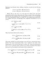
0
01 2 3 4
50
100
150
200
250
s
x
, s, MPa
e
x
, e, %
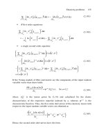
Fig. 4.9. Experimental stress–strain diagram for an aluminum alloy under uniaxial tension (solid line), the
universal stress–strain curve (dashed line) and its power approximation (dots).
curve σ(ε), we should put σ = σ
x

and change the scale on the strain axis in accordance
with Eq. (4.21). To do this, we need to know the plastic Poisson’s ratio ν
p
which can be
found from ν
p
=−ε
y
/ε
x
. Using Eqs. (4.29) and (4.30), we arrive at
ν
p
=
1
2
−
E
s
E

1
2
−ν

It follows from this equation that, ν
p
= ν if E
s
= E and ν

p
→ 1/2 for E
s
→ 0. The
dependencies of E
s
and ν
p
on ε for the aluminum alloy under consideration are presented
in Fig. 4.10. With the aid of this figure and Eq. (4.21) in which we should take ε
11
= ε
x
we can calculate ε and plot the universal curve shown in Fig. 4.9 with a dashed line. As
can be seen, this curve is slightly different from the diagram corresponding to a uniaxial
tension. For the power approximation in Eq. (4.27), we get from Eqs. (4.26) and (4.32)
the following equations
ω(σ) = Cnσ
n−2
, ω(σ) =
ε
σ
−
1
E
Matching these results, we find
ε =
σ
E
+Cnσ

n−1
(4.33)
146 Advanced mechanics of composite materials
0
01234
20
40
60
80
100
0
0.1
0.2
0.3
0.4
0.5
E
E
s
E
t
n
p
e
x
, %
n
p
Fig. 4.10. Dependencies of the secant modulus (E
s

), tangent modulus (E
t
), and the plastic Poisson’s ratio (ν
p
),
on strain for an aluminum alloy.
This is a traditional approximation for a material with a power hardening law. Now, we
can find C and n using Eq. (4.33) to approximate the dashed line in Fig. 4.9. The results
of this approximation are shown in this figure with dots that correspond to E = 71.4 GPa,
n = 6, and C = 6.23 ×10
−15
(MPa)
−5
.
Thus, constitutive equations of the deformation theory of plasticity are specified by
Eqs. (4.25) and (4.32). These equations are valid only for active loading that can be iden-
tified by the condition dσ>0. Being applied for unloading (i.e., for dσ<0), Eqs. (4.25)
correspond to nonlinear elastic material with stress–strain diagram shown in Fig. 1.2. For
an elastic–plastic material (see Fig. 1.5), the unloading diagram is linear. So, if we reduce
the stresses by some decrements σ
x
, σ
y
, and τ
xy
, the corresponding decrements of
strains will be
ε
x
=

1
E
(σ
x
−νσ
y
), ε
y
=
1
E
(σ
y
−νσ
x
), γ
xy
=
1
G
τ
xy
Direct application of the nonlinear equations (4.25) substantially hinders the problem of
stress–strain analysis because these equations include function ω(σ) in Eq. (4.32) which,
in turn, contains the secant modulus E
s
(σ ). For the power approximation corresponding
to Eq. (4.33), E
s
can be expressed analytically, i.e.,

1
E
s
=
1
E
+Cnσ
n−2
Chapter 4. Mechanics of a composite layer 147
However, in many cases E
s
is given graphically as in Fig. 4.10 or numerically in the
form of a table. Thus, Eqs. (4.25) sometimes cannot be even written in an explicit ana-
lytical form. This implies application of numerical methods in conjunction with iterative
linearization of Eqs. (4.25).
There exist several methods of such linearization that will be demonstrated using the
first equation in Eqs. (4.25), i.e.,
ε
x
=
1
E
(σ
x
−νσ
y
) +ω(σ)

σ
x

−
1
2
σ
y

(4.34)
In the method of elastic solutions (Ilyushin, 1948), Eq. (4.34) is used in the following
form
ε
s
x
=
1
E
(σ
s
x
−νσ
s
y
) +η
s−1
(4.35)
where s is the number of the iteration step and
η
s−1
= ω(σ
s−1
)


σ
s−1
x
−
1
2
σ
s−1
y

For the first step (s = 1), we take η
0
= 0 and solve the problem of linear elasticity with
Eq. (4.35) in the form
ε
1
x
=
1
E
(σ
1
x
−νσ
1
y
) (4.36)
Finding the stresses, we calculate η
1

and write Eq. (4.35) as
ε
2
x
=
1
E
(σ
2
x
−νσ
2
y
) +η
1
where the first term is linear, whereas the second term is a known function of coordinates.
Thus, we have another linear problem resolving which we find stresses, calculate η
2
, and
switch to the third step. This process is continued until the strains corresponding to some
step become sufficiently close within the stipulated accuracy to the results found at the
previous step.
Thus, the method of elastic solutions reduces the initial nonlinear problem to a sequence
of linear problems of the theory of elasticity for the same material but with some initial
strains that can be transformed into initial stresses or additional loads. This method read-
ily provides a nonlinear solution for any problem that has a linear solution, analytical
or numerical. The main shortcoming of the method is its poor convergence. Graphical
interpretation of this process for the case of uniaxial tension with stress σ is presented in
Fig. 4.11a. This figure shows a simple way to improve the convergence of the process.
148 Advanced mechanics of composite materials

(a) (b)
A
ee
s
A
s
(c) (d)
ee
A
s
A
s
Fig. 4.11. Geometric interpretation of (a) the method of elastic solutions, (b) the method of variable elasticity
parameters, (c) Newton’s method, and (d) method of successive loading.
If we need to find the strain at the point of the curve that is close to point A,itisnot
necessary to start the process with initial modulus E. Taking E

<Ein Eq. (4.36) we can
reach the result with much fewer steps.
According to the method of elastic variables (Birger, 1951), we should present
Eq. (4.34) as
ε
s
x
=
1
E
(σ
s
x

−νσ
s
y
) +ω(σ
s−1
)

σ
s
x
−
1
2
σ
s
y

(4.37)
In contrast to Eq. (4.35), stresses σ
s
x
and σ
s
y
in the second term correspond to the current
step rather than to the previous one. This enables us to write Eq. (4.37) in a form analogous
to Hooke’s law, i.e.,
ε
s
x

=
1
E
s−1
(σ
s
x
−ν
s−1
σ
s
y
) (4.38)
Chapter 4. Mechanics of a composite layer 149
where
E
s−1
=

1
E
+ω(σ
s−1
)

−1
,ν
s−1
= E
s−1


ν
E
+
1
2
ω(σ
s−1
)

(4.39)
are elastic variables corresponding to the step with number s −1. The iteration procedure
is similar to that described above. For the first step we take E
0
= E and ν
0
= ν in
Eq. (4.38). We then find σ
1
x
, σ
1
y
, and σ
1
, determine E
1
, ν
1
, switch to the second step

and so on. Graphical interpretation of the process is shown in Fig. 4.11b. Convergence of
this method is by an order faster than that of the method of elastic solutions. However,
elastic variables in the linear constitutive equation of the method, Eq. (4.38), depend
on stresses and hence, on coordinates whence the method has obtained its name. This
method can be efficiently applied in conjunction with the finite element method according
to which the structure is simulated with the system of elements with constant stiffness
coefficients. Being calculated for each step with the aid of Eqs. (4.39), these stiffnesses
will change only with transition from one element to another, which is as apparent would
not practically hinder the calculation procedure for the finite element method.
The iteration process having the best convergence is provided by the classical Newton’s
method requiring the following form of Eq. (4.34)
ε
s
x
= ε
s−1
x
+c
s−1
11

σ
s
x
−σ
s−1
x

+c
s−1

12

σ
s
y
−σ
s−1
y

+c
s−1
13

τ
s
xy
−τ
s−1
xy

(4.40)
where
c
s−1
11
=
1
E
+ω(σ
s−1

) +

σ
s−1
x
−
1
2
σ
s−1
y

∂
∂
σ
s−1
x
ω(σ
s−1
)
c
s−1
12
=−
ν
E
−
1
2
ω(σ

s−1
) +

σ
s−1
x
−
1
2
σ
s−1
y

∂
∂
σ
s−1
y
ω(σ
s−1
)
c
s−1
13
=

σ
s−1
x
−

1
2
σ
s−1
y

∂
∂
τ
s−1
xy
ω(σ
s−1
)
Since coefficients c are known from the previous step (s − 1), Eq. (4.40) is linear with
respect to stresses and strains corresponding to step number s. Graphical interpretation
of this method is presented in Fig. 4.11c. In contrast to the methods discussed above,
Newton’s method has no physical interpretation and being characterized with very high
convergence, is rather cumbersome for practical applications.
The iteration methods discussed above are used to solve direct problems of stress
analysis, i.e., to find stresses and strains induced by a given load. However, there
exists another class of problems requiring us to evaluate the load-carrying capacity of
the structure. To solve these problems, we need to trace the evolution of stresses while
the load increases from zero to some ultimate value. To do this, we can use the method of
150 Advanced mechanics of composite materials
successive loading. According to this method, the load is applied with some increments,
and for each s-step of loading the strain is determined as
ε
s
x

= ε
s−1
x
+
1
E
s−1

σ
s
x
−ν
s−1
σ
s
y

(4.41)
where E
s−1
and ν
s−1
are specified by Eqs. (4.39) and correspond to the previous loading
step. Graphical interpretation of this method is shown in Fig. 4.11d. To obtain reliable
results, the load increments should be as small as possible, because the error of calculation
is cumulative in this method. To avoid this effect, the method of successive loading can
be used in conjunction with the method of elastic variables. Being applied after several
loading steps (black circles in Fig. 4.11d) the latter method allows us to eliminate the
accumulated error and to start again the process of loading from a ‘correct’ initial state
(light circles in Fig. 4.11d).

Returning to the constitutive equations of the deformation theory of plasticity,
Eq. (4.25), it is important to note that these equations are algebraic. This means that strains
corresponding to some combination of loads are determined by the stresses induced by
these loads and do not depend on the history of loading, i.e., on what happened to the
material before this combination of loads was reached.
However, existing experimental data show that, in general, strains should depend on
the history of loading. This means that constitutive equations should be differential rather
than algebraic as they are in the deformation theory. Such equations are provided by the
flow theory of plasticity. According to this theory, decomposition in Eq. (4.15) is used for
infinitesimal increments of stresses, i.e.,
dε
ij
= dε
e
ij
+dε
p
ij
(4.42)
Here, increments of elastic strains are related to the increments of stresses by Hooke’s
law, e.g., for the plane stress state
dε
e
x
=
1
E
(dσ
x
−νdσ

y
), dε
e
y
=
1
E
(dσ
y
−νdσ
x
), dγ
xy
=
1
G
dτ
xy
(4.43)
whereas increments of plastic strains
dε
p
ij
=
∂
U
p
∂
σ
ij

dλ
are expressed in the form of Eq. (4.18) but include a parameter λ which characterizes the
loading process.
Assuming that U
p
= U
p
(σ ), where σ is the stress intensity specified by Eq. (4.19) or
(4.24), we get
dε
p
ij
=
dU
p
dσ
∂
σ
∂
σ
ij
dλ
Chapter 4. Mechanics of a composite layer 151
The explicit form of these equations for the plane stress state is
dε
p
x
= dω(σ)

σ

x
−
1
2
σ
y

dε
p
y
= dω(σ)

σ
y
−
1
2
σ
x

(4.44)
dγ
p
xy
= 3dω(σ)τ
xy
where
dω(σ) =
1
σ

dU
p
dσ
dλ (4.45)
To determine the parameter λ, assume that the plastic potential U
p
, being on the one hand
a function of σ , can be treated as the work performed by stresses on plastic strains, i.e.,
dU
p
=
∂
U
p
∂
σ
dσ
= σ
x
dε
p
x
+σ
y
dε
p
y
+τ
xy
dγ

p
xy
Substituting strain increments from Eqs. (4.44) and taking into account Eq. (4.24) for σ ,
we have
∂
U
p
∂
σ
dσ = σ
2
dω(σ)
With due regard to Eq. (4.45), we arrive at the following simple and natural relationship
dλ = dσ/σ. Thus, Eq. (4.45) takes the form
dω(σ) =
dσ
σ
2
dU
p
dσ
(4.46)
and Eqs. (4.42)–(4.44) result in the following constitutive equations for the flow theory
dε
x
=
1
E
(dσ
x

−νdσ
y
) +dω(σ)

σ
x
−
1
2
σ
y

dε
y
=
1
E
(dσ
y
−νdσ
x
) +dω(σ)

σ
y
−
1
2
σ
x


dγ
xy
=
1
G
dτ
xy
+3dω(σ)τ
xy
(4.47)
As can be seen, in contrast to the deformation theory, stresses govern the increments of
plastic strains rather than the strains themselves.