ADVANCED MECHANICS OF COMPOSITE MATERIALS Episode 6 ppt

162 Advanced mechanics of composite materials
As an example, consider a boron–aluminum unidirectional composite whose experi-
mental stress–strain diagrams (Herakovich, 1998) are shown in Fig. 4.17 (circles) along
with the corresponding approximations (solid lines) plotted with the aid of Eqs. (4.65).
4.3. Unidirectional anisotropic layer
Consider now a unidirectional layer studied in the previous section and assume that its
principal material axis 1 makes some angle φ with the x-axis of the global coordinate
frame (see Fig. 4.18). An example of such a layer is shown in Fig. 4.19.
4.3.1. Linear elastic model
Constitutive equations of the layer under study referred to the principal material coor-
dinates are given by Eqs. (4.55) and (4.56). We need now to derive such equations for
the global coordinate frame x, y, and z (see Fig. 4.18). To do this, we should transfer
stresses σ
1
, σ
2
, τ
12
, τ
13
, τ
23
acting in the layer and the corresponding strains ε
1
, ε
2
, γ
12
,
γ
13

, γ
23
into stress and strain components σ
x
, σ
y
, τ
xy
, τ
xz
, τ
yz
and ε
x
, ε
y
, γ
xy
, γ
xz
, γ
yz
using Eqs. (2.8), (2.9) and (2.21), (2.27) for coordinate transformation of stresses and
strains. According to Fig. 4.18, the directional cosines, Eqs. (2.1), for this transformation
are (we take x

= 1, y

= 2, z


= 3)
l
x
1
x
= c, l
x
1
y
= s, l
x
1
z
= 0
l
y
1
x
=−s, l
y
1
y
= c, l
y
1
z
= 0
l
z
1

x
= 0,l
z
1
y
= 0,l
z
1
z
= 1
(4.66)
where c = cos φ and s = sin φ. Using Eqs. (2.8) and (2.9), we get
σ
1
= σ
x
c
2
+σ
y
s
2
+2τ
xy
cs
σ
2
= σ
x
s

2
+σ
y
c
2
−2τ
xy
cs
τ
12
= (σ
y
−σ
x
)cs +τ
xy

c
2
−s
2

τ
13
= τ
xz
c +τ
yz
s
τ

12
=−τ
xz
s +τ
yz
c
(4.67)
The inverse form of these equations is
σ
x
= σ
1
c
2
+σ
2
s
2
−2τ
12
cs
σ
y
= σ
1
s
2
+σ
2
c

2
+2τ
12
cs
Chapter 4. Mechanics of a composite layer 163
−300
−250
−200
−150
−100
−50
50
100
150
−2 −1.8 −1.6 −1.4 −1.2 −1 −0.8 −0.6 −0.4 −0.2
0
0.2
(a)
(b)
0
012345678
20
40
60
80
100
120
140
t
12

, MPa
g
12
, %
e
2
, %
s
2
, MPa
Fig. 4.17. Calculated (solid lines) and experimental (circles) stress–strain diagrams for a boron–aluminum
composite under transverse loading (a) and in-plane shear (b).
164 Advanced mechanics of composite materials
t
23
t
yz
t
xz
t
xy
t
13
s
1
s
y
s
x
s

2
t
12
f
2
3
1
z
y
x
Fig. 4.18. A composite layer consisting of a system of unidirectional plies with the same orientation.
Fig. 4.19. An anisotropic outer layer of a composite pressure vessel. Courtesy of CRISM.
τ
xy
= (σ
1
−σ
2
)cs +τ
12

c
2
−s
2

(4.68)
τ
xz
= τ

13
c −τ
23
s
τ
yz
= τ
13
s +τ
23
c
The corresponding transformation for strains follows from Eqs. (2.21) and (2.27), i.e.,
ε
1
= ε
x
c
2
+ε
y
s
2
+γ
xy
cs
ε
2
= ε
x
s

2
+ε
y
c
2
−γ
xy
cs
Chapter 4. Mechanics of a composite layer 165
γ
12
= 2(ε
y
−ε
x
)cs +γ
xy

c
2
−s
2

(4.69)
γ
13
= γ
xz
c +γ
yz

s
γ
23
=−γ
xz
s +γ
yz
c
or
ε
x
= ε
1
c
2
+ε
2
s
2
−γ
12
cs
ε
y
= ε
1
s
2
+ε
2

c
2
+γ
12
cs
γ
xy
= 2(ε
1
−ε
2
)cs +γ
12

c
2
−s
2

γ
xz
= γ
13
c −γ
23
s
γ
yz
= γ
13

s +γ
23
c
(4.70)
To derive constitutive equations for an anisotropic unidirectional layer, we substitute
strains, Eqs. (4.69), into Hooke’s law, Eqs. (4.56), and the derived stresses – into
Eqs. (4.68). The final result is as follows
σ
x
= A
11
ε
x
+A
12
ε
y
+A
14
γ
xy
σ
y
= A
21
ε
x
+A
22
ε

y
+A
24
γ
xy
τ
xy
= A
41
ε
x
+A
42
ε
y
+A
44
γ
xy
τ
xz
= A
55
γ
xz
+A
56
γ
yz
τ

yz
= A
65
γ
xz
+A
66
γ
yz
(4.71)
The stiffness coefficients in these equations are
A
11
= E
1
c
4
+E
2
s
4
+2E
12
c
2
s
2
A
12
= A

21
= E
1
ν
12
+(E
1
+E
2
−2E
12
)c
2
s
2
A
14
= A
41
=

E
1
c
2
−E
2
s
2
−E

12

c
2
−s
2


cs
A
22
= E
1
s
4
+E
2
c
4
+2E
12
c
2
s
2
A
24
= A
42
=


E
1
s
2
−E
2
c
2
+E
12

c
2
−s
2


cs (4.72)
A
44
= (E
1
+E
2
−2E
1
ν
12
)c

2
s
2
+G
12

c
2
−s
2

2
A
55
= G
13
c
2
+G
23
s
2
A
56
= A
65
= (G
13
−G
23

)cs
A
66
= G
13
s
2
+G
23
c
2
166 Advanced mechanics of composite materials
where
E
1, 2
=
E
1, 2
1 −ν
12
ν
21
,E
12
= E
1
ν
12
+2G
12

,c= cos φ, s = sin φ
The dependence of stiffness coefficients A
mn
in Eqs. (4.72) on φ has been studied by
Tsai and Pagano (see, e.g., Tsai, 1987; Verchery, 1999). Changing the powers of sin φ
and cos φ in Eqs. (4.72) for multiple-angle trigonometric functions, we can reduce these
equations to the following form (Verchery, 1999)
A
11
= S
1
+S
2
+2S
3
cos 2φ +S
4
cos 4φ
A
12
=−S
1
+S
2
−S
4
cos 4φ
A
14
= S

3
sin 2φ +S
4
sin 4φ
A
22
= S
1
+S
2
− 2S
3
cos 2φ +S
4
cos 4φ
A
24
= S
3
sin 2φ −S
4
sin 4φ
A
44
= S
1
−S
4
cos 4φ
A

55
= S
5
+S
6
cos 2φ
A
56
= 4S
6
sin 2φ
A
66
= S
5
−S
6
cos 2φ
(4.73)
In these equations,
S
1
=
1
8

A
0
11
+A

0
22
−2A
0
12
+4A
0
44

S
2
=
1
4

A
0
11
+A
0
22
+2A
0
12

S
3
=
1
4


A
0
11
−A
0
22

S
4
=
1
8

A
0
11
+A
0
22
−2A
0
12
−4A
0
44

S
5
=

1
2

A
0
55
+A
0
66

S
6
=
1
2

A
0
55
−A
0
66

Chapter 4. Mechanics of a composite layer 167
where A
0
n
are stiffness coefficients corresponding to φ = 0. It follows from Eqs. (4.72)
that,
A

0
11
= E
1
,A
0
12
= E
1
ν
12
,A
0
14
= A
0
24
= A
0
56
= 0
A
0
22
= E
2
,A
0
44
= G

12
,A
0
55
= G
13
,A
0
66
= G
23
As can be seen in Eqs. (4.73), there exist the following differential relationships between
tensile and coupling stiffnesses (Verchery and Gong, 1999)
dA
11
dφ
=−4A
14
,
dA
22
dφ
= 4A
24
It can be directly checked that Eqs. (4.73) provide three invariant stiffness characteristics
whose forms do not depend on φ, i.e.,
A
11
(φ) +A
22

(φ) +2A
12
(φ) = A
0
11
+A
0
22
+2A
0
12
A
44
(φ) −A
12
(φ) = A
0
44
−A
0
12
A
55
(φ) +A
66
(φ) = A
0
55
+A
0

66
(4.74)
Any linear combination of these equations is also an invariant combination of stiffness
coefficients.
The inverse form of Eqs. (4.71) can be obtained if we substitute stresses, Eqs. (4.67),
into Hooke’s law, Eqs. (4.55), and the derived strains in Eqs. (4.70). As a result, we arrive
at the following particular form of Eqs. (2.48) and (2.49)
ε
x
=
σ
x
E
x
−ν
xy
σ
y
E
y
+η
x,xy
τ
xy
G
xy
,ε
y
=
σ

y
E
y
−ν
yx
σ
x
E
x
+η
y,xy
τ
xy
G
xy
γ
xy
=
τ
xy
G
xy
+η
xy, x
σ
x
E
x
+η
xy, y

σ
y
E
y
,γ
xz
=
τ
xz
G
xz
+λ
xz,yz
τ
yz
G
yz
γ
yz
=
τ
yz
G
yz
+λ
yz,xz
τ
xz
G
xz

(4.75)
in which the compliance coefficients are
1
E
x
=
c
4
E
1
+
s
4
E
2
+

1
G
12
−
2ν
21
E
1

c
2
s
2

ν
xy
E
y
=
ν
yx
E
x
=
ν
21
E
1
−

1
E
1
+
1
E
2
+
ν
21
E
1
−
1

G
12

c
2
s
2
η
x,xy
G
xy
=
η
xy,x
E
x
=2

c
2
E
1
−
s
2
E
2
−

1

2G
12
−
ν
21
E
1


c
2
−s
2


cs
168 Advanced mechanics of composite materials
1
E
y
=
s
4
E
1
+
c
4
E
2

+

1
G
12
−
2ν
21
E
1

c
2
s
2
(4.76)
η
y,xy
G
xy
=
η
xy,y
E
y
=2

s
2
E

1
−
c
2
E
2
+

1
2G
12
−
ν
21
E
1


c
2
−s
2


cs
1
G
xy
=4


1
E
1
+
1
E
2
+
2ν
21
E
1

c
2
s
2
+
1
G
12

c
2
−s
2

2
1
G

xz
=
c
2
G
13
+
s
2
G
23
,
λ
xz,yz
G
yz
=
λ
yz,xz
G
xz
=

1
G
13
−
1
G
23


cs,
1
G
yz
=
s
2
G
13
+
c
2
G
23
There exist the following dependencies between the coefficients of Eqs. (4.71) and (4.75)
1
E
x
=
1
D
1

A
22
A
44
−A
2

24

,
ν
xy
E
y
=
ν
yx
E
x
=
1
D
1
(A
12
A
44
−A
14
A
24
)
η
x,xy
G
xy
=

η
xy,x
E
x
=
1
D
1
(
A
12
A
24
−A
22
A
14
)
,
1
E
y
=
1
D
1

A
11
A

44
−A
2
14

η
y,xy
G
xy
=
η
xy,y
E
y
=
1
D
1
(A
12
A
14
−A
11
A
24
),
1
G
xy

=
1
D
1

A
11
A
22
−A
2
12

1
G
xz
=
A
66
D
2
,
1
G
yz
=
A
55
D
2

,
λ
xz,yz
G
yz
=
λ
yz,xz
G
xz
=−
A
56
D
2
Here,
D
1
= A
11
A
22
A
44
−A
11
A
2
24
−A

22
A
2
14
−A
44
A
2
12
+2A
12
A
14
A
24
D
2
= A
55
A
66
−A
2
56
and
A
11
=
1 −η
y,xy

η
xy, y
D
3
E
y
G
xy
,A
12
=
ν
xy
−η
x,xy
η
xy, y
D
3
E
y
G
xy
A
14
=−
η
x,xy
+ν
xy

η
y,xy
D
3
E
y
G
xy
,A
22
=
1 −η
x,xy
η
xy, y
D
3
E
x
G
xy
A
24
=−
η
y,xy
+ν
yx
η
x,xy

D
3
E
x
G
xy
,A
44
=
1 −ν
xy
ν
yx
D
3
E
x
E
y
A
55
=
1
D
4
G
yz
,A
56
=−

λ
xz,yz
D
4
G
yz
,A
66
=
1
D
4
G
xz
Chapter 4. Mechanics of a composite layer 169
where
D
3
=
1
E
x
E
y
G
xy
(1 −ν
xy
ν
yx

−η
x,xy
η
xy, x
−η
y,xy
η
xy, y
−ν
xy
η
y,xy
η
xy, x
−ν
yx
η
x,xy
η
xy, y
)
D
4
=
1
G
xz
G
yz
(1 −λ

xz,yz
λ
yz,xz
)
As can be seen in Eqs. (4.71) and (4.75), the layer under study is anisotropic in plane
xy because the constitutive equations include shear–extension and shear–shear coupling
coefficients η and λ. For φ = 0, the foregoing equations degenerate into Eqs. (4.55) and
(4.56) for an orthotropic layer.
The dependencies of stiffness coefficients on the orientation angle for a carbon–epoxy
composite with properties listed in Table 3.5 are presented in Figs. 4.20 and 4.21.
Uniaxial tension of the anisotropic layer (the so-called off-axis test of a unidirectional
composite) is often used to determine material characteristics that cannot be found in
tests with orthotropic specimens or to evaluate constitutive and failure theories. Such a
0
0 153045607590
20
40
60
80
100
120
140
A
mn
, GPa
A
11
A
22
A

44
f°
Fig. 4.20. Dependencies of tensile (A
11
, A
22
) and shear (A
44
) stiffnesses of a unidirectional carbon–epoxy layer
on the orientation angle.
170 Advanced mechanics of composite materials
0
0 153045607590
10
20
30
40
A
12
A
14
A
mn
, GPa
A
24

f°
Fig. 4.21. Dependencies of coupling stiffnesses of a unidirectional carbon–epoxy layer on the orientation angle.
test is shown in Fig. 4.22. To study this loading case, we should take σ

y
= τ
xy
= 0in
Eqs. (4.75). Then,
ε
x
=
σ
x
E
x
,ε
y
=−ν
xy
σ
x
E
x
,γ
xy
= η
xy, x
σ
x
E
x
(4.77)
As can be seen in these equations, tension in the x-direction is accompanied not only

with transverse contraction, as in orthotropic materials, but also with shear. This results
in the deformed shape of the sample shown in Fig. 4.23. This shape is natural because
the material stiffness in the fiber direction is much higher than that across the fibers.
Such an experiment, in cases where it can be performed, allows us to determine the
in-plane shear modulus, G
12
in principle material coordinates using a simple tensile test
rather than the much more complicated tests described in Section 3.4.3 and shown in
Figs. 3.54 and 3.55. Indeed, if we know E
x
from the tensile test in Fig. 4.23 and find E
1
,
E
2
, and ν
21
from tensile tests along and across the fibers (see Sections 3.4.1 and 3.4.2),
we can use the first equation of Eqs. (4.76) to determine
G
12
=
sin
2
φ cos
2
φ
(
1/E
x

)
−

cos
4
φ/E
1

−

sin
4
φ/E
2

+
(
2ν
21
/E
1
)
sin
2
φ cos
2
φ
(4.78)
In connection with this, a question arises as to what angle should be substituted into this
equation to provide the most accurate result. The answer is given in Fig. 4.24, which

displays the strains in principal material coordinates for a carbon–epoxy layer calculated
with the aid of Eqs. (4.69) and (4.77). As can be seen in this figure, the most appropriate
angle is about 10
◦
. At this angle, the shear strain γ
12
is much higher than normal strains
ε
1
and ε
2
, so that material deformation is associated mainly with shear. An off-axis test
Chapter 4. Mechanics of a composite layer 171
Fig. 4.22. An off-axis test.
s
x
s
x
g
g

Fig. 4.23. Deformation of a unidirectional layer loaded at an angle to fiber orientation.
172 Advanced mechanics of composite materials
0
0 153045607590
0.5
1
1.5
2
2.5

3
e
1
/e
x
, e
2
/e
x
, g
12
/e
x
e
2
/e
x
e
1
/e
x
g
12
/e
x
f°
Fig. 4.24. Dependencies of normalized strains in the principle material coordinates on the angle of the
off-axis test.
with φ = 10
◦

can also be used to evaluate material strength in shear τ
12
(Chamis, 1979).
Stresses acting under off-axis tension in the principal material coordinates are statically
determinate and can be found directly from Eqs. (4.67) as
σ
1
= σ
x
cos
2
φ, σ
2
= σ
x
sin
2
φ, τ
12
=−σ
x
sin φ cos φ (4.79)
Thus, applying stress σ
x
and changing φ we can induce proportional loading with different
combinations of stresses σ
1
, σ
2
, and τ

12
to evaluate putative constitutive or failure theories
for a material under study.
However, the test shown in Fig. 4.23 can hardly be performed because the test fixture
(see Fig. 4.22) restrains the shear deformation of the specimen and induces a corresponding
shear stress. The constitutive equations for the specimen loaded with uniaxial tension as
in Fig. 4.23 and fixed as in Fig. 4.22 follow from Eqs. (4.75) if we take σ
y
= 0, i.e.,
ε
x
=
σ
x
E
x
+η
x, xy
τ
xy
G
xy
(4.80)
γ
xy
=
τ
xy
G
xy

+η
xy, x
σ
x
E
x
(4.81)
Chapter 4. Mechanics of a composite layer 173
in which elastic constants are specified by Eqs. (4.76). The shear stress, being of a reactive
nature, can be found from Eq. (4.81) if we put γ
xy
= 0. Then,
τ
xy
=−η
xy, x
G
xy
E
x
σ
x
Substituting this result into Eq. (4.80), we arrive at
ε
x
=
σ
x
E
a

x
(4.82)
Here,
E
a
x
=
E
x
1 −η
x, xy
η
xy, x
(4.83)
is the apparent elastic modulus that can be found from the test shown in Fig. 4.22. As
follows from Eq. (4.83), E
a
x
, in general, does not coincide with E
x
as used in Eq. (4.78)
for G
12
.
Thus, measuring σ
x
and ε
x
we can determine E
x

from Eq. (4.82) only under the condi-
tion E
a
x
= E
x
, which means that the shear–extension coupling coefficient η must be zero.
Applying Eqs. (4.76) and assuming that φ = 0 and φ = 90
◦
, we arrive at the following
condition providing η = 0
sin
2
φ
0
=
e
1
e
2
(4.84)
in which
e
1
=
1 +ν
21
E
1
−

1
2G
12
,e
2
=
1 +ν
21
E
1
+
1 +ν
12
E
2
−
1
G
12
Since 0 ≤ sin
2
φ ≤ 1, there exist two cases in which Eq. (4.84) is valid. The first case
corresponds to the following set of inequalities
e
1
≥ 0,e
2
> 0,e
2
≥ e

1
(4.85)
whereas for the second case,
e
1
≤ 0,e
2
< 0,e
2
≤ e
1
(4.86)
To be specific, suppose that E
1
>E
2
. Then, taking into account the symmetry condition
ν
12
E
1
= ν
21
E
2
we have
1 +ν
12
E
2

>
1 +ν
21
E
1
(4.87)
174 Advanced mechanics of composite materials
Consider the first set of inequalities in Eqs. (4.85) and assume that the first of them, which
has the following explicit form
1 +ν
21
E
1
≥
1
2G
12
(4.88)
is valid. Then, Eq. (4.87) yields
1 +ν
12
E
2
>
1 +ν
21
E
1
≥
1

2G
12
or
1 +ν
12
E
2
>
1
2G
12
Matching this result with the last inequality in Eqs. (4.85) presented in the form
1 +ν
12
E
2
≥
1
2G
12
(4.89)
we can conclude that if the first condition in Eqs. (4.85) is valid, then the last of these
conditions is valid too.
Consider the second condition in Eqs. (4.85) and write it in explicit form, i.e.,
1 +ν
12
E
2
+
1 +ν

21
E
1
≥
1
G
12
(4.90)
Transforming Eq. (4.87) and using Eq. (4.89), we have
1 +ν
12
E
2
+
1 +ν
21
E
1
> 2
1 +ν
21
E
1
≥
1
G
12
which means that the condition in Eq. (4.90) is valid.
So, the set of conditions in Eqs. (4.85) can be reduced to one inequality in Eq. (4.88),
which can be written in a final form as

G
12
≥
E
1
2(1 +ν
21
)
(4.91)
Consider conditions (4.86) and assume that the last of them, which can be presented in
the following explicit form
1 +ν
12
E
2
≤
1
2G
12
(4.92)
is valid. Using Eqs. (4.87) and (4.92), we get
1 +ν
21
E
1
<
1 +ν
12
E
2

≤
1
2G
12
or
1 +ν
21
E
1
<
1
2G
12
Chapter 4. Mechanics of a composite layer 175
Since the first condition in Eqs. (4.86) can be presented as
1 +ν
21
E
1
≤
1
2G
12
we can conclude that it is satisfied.
Consider the second inequality in Eqs. (4.86) and write it in an explicit form, i.e.,
1 +ν
21
E
1
+

1 +ν
12
E
2
<
1
G
12
(4.93)
Using Eqs. (4.87) and (4.92), we get
1 +ν
21
E
1
+
1 +ν
12
E
2
< 2
1 +ν
12
E
2
≤
1
G
12
which means that the condition in Eq. (4.93) is satisfied.
So, the set of conditions in Eqs. (4.86) is reduced to one inequality in Eq. (4.92), which

can be written in the following final form
G
12
≤
E
2
2(1 +ν
12
)
(4.94)
Thus, Eq. (4.84) determines the angle φ
0
for the orthotropic materials whose mechanical
characteristics satisfy the conditions in Eqs. (4.91) or (4.94). Such materials, being loaded
at an angle φ = φ
0
, do not experience shear–stretching coupling. The shear modulus can
be found from Eq. (4.78) in which E
x
= σ
x
/ε
x
, where σ
x
and ε
x
are the stress and the
strain determined in the off-axis tension test shown in Fig. 4.22.
Consider as examples unidirectional composites with typical properties (Table 3.5).

(1) For fiberglass–epoxy composite, we have E
1
= 60 GPa, E
2
= 13 GPa,
G
12
= 3.4 GPa, ν
12
= 0.065, ν
21
= 0.3
Calculation in accordance with Eqs. (4.91) and (4.94) yields
E
1
2(1 +ν
21
)
= 23.08 GPa,
E
2
2(1 +ν
12
)
= 6.1 GPa
Thus, the condition in Eq. (4.94) is satisfied, and Eq. (4.84) gives φ
0
= 54.31
◦
.

(2) For aramid–epoxy composite, E
1
= 95 GPa, E
2
= 5.1 GPa, G
12
= 1.8 GPa,
ν
12
= 0.018, ν
21
= 0.34
E
1
2(1 +ν
21
)
= 36.45 GPa,
E
2
2(1 +ν
12
)
= 2.5 GPa, and φ
0
= 61.45
◦
(3) For carbon–epoxy composite with E
1
= 140 GPa, E

2
= 11 GPa, G
12
= 5.5 GPa,
ν
12
= 0.021, ν
21
= 0.27, we have
E
1
2(1 +ν
21
)
= 55.12 GPa,
E
2
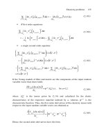
2(1 +ν
12
)
= 5.39 GPa
176 Advanced mechanics of composite materials
As can be seen, the conditions in Eqs. (4.91) and (4.94) are not satisfied, and angle φ
0
does not exist for this material.
As can be directly checked with the aid of Eqs. (4.76), there exists the following rela-
tionship between the elastic constants of anisotropic materials (Verchery and Gong, 1999)
d
dφ


1
E
x

=−2
η
x, xy
G
xy
This equation means that η
x, xy
= 0 for materials whose modulus E
x
reaches the extremum
value in the interval 0 <φ<90
◦
. The dependencies of E
x
/E
1
on φ for the materials
considered above as examples, are shown in Fig. 4.25.
As can be seen, curves 1 and 2 corresponding to glass and aramid composites reach
the minimum value at φ
0
= 54.31
◦
and φ
0
= 61.45

◦
, respectively, whereas curve 3 for
carbon composite does not have a minimum at 0 <φ<90
◦
.
The dependence E
x
(φ) with the minimum value of E
x
reached at φ = φ
0
, where
0 <φ<90
◦
, is typical for composites reinforced in two orthogonal directions. For
example, for a fabric composite having E
1
= E
2
and ν
12
= ν
21
, Eq. (4.84) yields the
well-known result φ
0
= 45
◦
. For a typical fiberglass fabric composite with E
1

= 26 GPa,
E
2
= 22 GPa, G
12
= 7.2 GPa, ν
12
= 0.11, ν
21
= 0.13, we have
E
1
2(1 +ν
21
)
= 11.5 GPa,
E
2
2(1 +ν
12
)
= 9.9 GPa, and φ
0
= 49.13
◦
0
0 102030405060708090
0.1
0.2
0.3

0.4
0.5
0.6
0.7
0.8
0.9
1
E
1
E
x
1
2
f = 54.31° f = 61.45°
f
°
3
Fig. 4.25. Dependencies of E
x
/E
1
on φ for fiberglass (1), aramid (2) and carbon (3) epoxy composites.
Chapter 4. Mechanics of a composite layer 177
In conclusion, it should be noted that the actual application of Eq. (4.78) is hindered by
the fact that the angle φ
0
specified by Eq. (4.84) depends on G
12
, which is not known and
needs to be determined from Eq. (4.78). To find G

12
, we actually need to perform several
tests for several values of G
12
in the vicinity of the expected value and the corresponding
values of φ
0
following from Eq. (4.84) and to select the correct value of G
12
, which
satisfies in conjunction with the corresponding value of φ
0
, both equations – Eqs. (4.78)
and (4.84) (Morozov and Vasiliev, 2003).
Consider the general case of an off-axis test (see Fig. 4.22) for a composite specimen
with an arbitrary fiber orientation angle φ (see Fig. 4.26). To describe this test, we need
to study the coupled problem for an anisotropic strip in which shear is induced by tension
but is restricted at the strip ends by the jaws of a test frame as in Figs. 4.22 and 4.26.
As follows from Fig. 4.26, the action of the grip can be simulated if we apply a bending
moment M and a transverse force V such that the rotation of the strip ends (γ in Fig. 4.23)
will become zero. As a result, bending normal and shear stresses appear in the strip that
can be analyzed with the aid of composite beam theory (Vasiliev, 1993).
To derive the corresponding equations, introduce the conventional assumptions of beam
theory according to which axial, u
x
, and transverse, u
y
, displacements can be presented as
u
x

= u(x) +yθ, u
y
= v(x)
where u and θ are the axial displacement and the angle of rotation of the strip cross section
x = constant and v is the strip deflection in the xy-plane (see Fig. 4.26). The strains
corresponding to these displacements follow from Eqs. (2.22), i.e.,
ε
x
=
∂
u
x
∂
x
= u

+yθ

= ε + yθ

γ
xy
=
∂
u
x
∂
y
+
∂

u
y
∂
x
= θ +v

(4.95)
where
()

= d
()
/dx and ε is the elongation of the strip axis. These strains are related
to stresses by Eqs. (4.75) which reduce to
ε
x
=
σ
x
E
x
+η
x, xy
τ
xy
G
xy
γ
xy
=

τ
xy
G
xy
+η
xy, x
σ
x
E
x
(4.96)
y
x
a
l
V
M
ss
Fig. 4.26. Off-axis tension of a strip fixed at the ends.
178 Advanced mechanics of composite materials
The inverse form of these equations is
σ
x
= B
11
ε
x
+B
14
γ

xy
,τ
xy
= B
41
ε
x
+B
44
γ
xy
(4.97)
where
B
11
=
E
x
1 −η
x, xy
η
xy,x
,B
44
=
G
xy
1 −η
x, xy
η

xy, x
B
14
= B
41
=−
E
x
η
x, xy
1 −η
x, xy
η
xy, x
=−
G
xy
η
xy, x
1 −η
x, xy
η
xy, x
(4.98)
Now, decompose the strip displacements, strains, and stresses into two components
corresponding to
(1) free tension (see Fig. 4.23), and
(2) bending.
For free tension, we have τ
xy

= 0 and v = 0. So, Eqs. (4.95) and (4.96) yield
ε
(1)
x
= ε
1
+yθ

1
,γ
(1)
xy
= θ
1
ε
(1)
x
=
σ
(1)
x
E
x
,γ
(1)
xy
= η
xy, x
σ
(1)

x
E
x
(4.99)
Here, ε
1
= u

1
and σ
(1)
x
= σ = F/ah, where F is the axial force applied to the strip,
a the strip width, and h is its thickness. Since σ
(1)
x
= constant, Eqs. (4.99) give
θ
1
= η
xy, x
σ
E
x
= constant, ε
1
x
= ε
1
=

σ
E
x
=
F
ah
(4.100)
Adding components corresponding to bending (with index 2), we can write the total
displacements and strains as
u
x
= u
1
+u
2
+y(θ
1
+θ
2
), u
y
= v
2
ε
x
= ε
1
+ε
2
+yθ


2
,γ
xy
= θ
1
+θ
2
+v

2
The total stresses can be expressed with the aid of Eqs. (4.97), i.e.,
σ
x
= B
11

ε
1
+ε
2
+yθ

2

+B
14

θ
1

+θ
2
+v

2

τ
xy
= B
41

ε
1
+ε
2
+yθ

2

+B
44

θ
1
+θ
2
+v

2


Transforming these equations with the aid of Eqs. (4.98) and (4.100), we arrive at
σ
x
= σ + B
11

ε
2
+yθ

2

+B
14

θ
2
+v

2

τ
xy
= B
41

ε
2
+yθ


2

+B
44
(θ
2
+v

2
)
(4.101)
Chapter 4. Mechanics of a composite layer 179
These stresses are statically equivalent to the axial force P , the bending moment M, and
the transverse force V , which can be introduced as
P = h

a/2
−a/2
σ
x
dy, M = h

a/2
−a/2
σ
x
ydy, V = h

a/2
−a/2

τ
xy
dy
Substitution of Eqs. (4.101) and integration yields
P = ah

σ + B
11
ε
2
+B
14

θ
2
+v

2

, (4.102)
M = B
11
h
a
3
12
θ

2
(4.103)

V = ah

B
41
ε
2
+B
44

θ
2
+v

2

(4.104)
These forces and moments should satisfy the equilibrium equation that follows from
Fig. 4.27, i.e.,
P

= 0,V

= 0,M

= V (4.105)
Solution of the first equation is P = F = σah. Then, Eq. (4.102) gives
ε
2
=−
B

14
B
11

θ
2
+v

2

(4.106)
The second equation of Eqs. (4.105) shows that V = C
1
, where C
1
is a constant of
integration. Then, substituting this result into Eq. (4.104) and eliminating ε
2
with the aid
of Eq. (4.106), we have
θ
2
+v

2
=
C
1
ahB
44

(4.107)
where
B
44
= B
44
−B
14
B
41
.
Taking in the third equation of Eqs. (4.105) V = C
1
and substituting M from
Eq. (4.103), we arrive at the following equation for θ
2
θ

2
=
12C
1
a
3
hB
11
P
M
V
dx

P + P ′ d
x
V + V ′ dx
M + M ′ dx
Fig. 4.27. Forces and moments acting on the strip element.
180 Advanced mechanics of composite materials
Integration yields
θ
2
=
6C
1
a
3
hB
11
+C
2
x +C
3
The total angle of rotation θ = θ
1
+θ
2
, where θ
1
is specified by Eqs. (4.100), should be
zero at the ends of the strip, i.e., θ(x =±l/2) = 0. Satisfying these conditions, we have
θ
2

=
3C
1
a
3
hB
11

2x
2
−
l
2
2

−η
xy, x
σ
E
x
(4.108)
Substitution into Eq. (4.107) and integration allows us to find the deflection
v
2
=
C
1
x
ahB
44

−
3C
1
x
a
3
hB
11

2x
2
3
−
l
2
2

+η
xy, x
σ
0
x
E
x
+C
4
(4.109)
This expression includes two constants, C
1
and C

4
, which can be determined from the
boundary conditions v
2
(x =±l/2) = 0. The final result, following from Eqs. (4.100),
(4.108), and (4.109), is
v = lη
xy, x
σ x
E
x

1 −
B
11
+l
2
B
44

3/2 −2
x
2

B
11
+l
2
B
44


θ = η
xy, x
3σ l
2
E
x
B
44

2
x
2
−1/2

B
11
+l
2
B
44
(4.110)
where
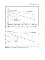
l = l/a and x = x/l. The deflection of a carbon–epoxy strip having φ = 45
◦
and
l = 10 is shown in Fig. 4.28.
0
−0.1
−0.05

0.05
0.1
−0.5 −0.4 −0.3 −0.2 −0.1 0.1 0.2 0.3 0.4 0.5
vE
x
ls
x
l
Fig. 4.28. Normalized deflection of a carbon–epoxy strip (φ = 45
◦
, l = 10).
Chapter 4. Mechanics of a composite layer 181
Now, we can write the relationship between modulus E
x
corresponding to the ideal test
shown in Fig. 4.23 and apparent modulus E
a
x
that can be found from the real test shown
in Figs. 4.22 and 4.26. Using Eqs. (4.98), (4.100), (4.106), and (4.110), we finally get
σ = E
a
x
ε
where
E
a
x
=
E

x
1 −

E
x
η
x, xy
η
xy, x

E
x
+l
2
G
xy
(1 −η
x, xy
η
xy, x
)

Consider two limiting cases. For an infinitely long strip (
l →∞), we have E
a
x
= E
x
. This
result corresponds to the case of free shear deformation specified by Eqs. (4.77). For an

infinitely short strip (
l → 0), taking into account Eqs. (4.98), we get
E
a
x
=
E
x
1 −η
x,xy
η
xy, x
= B
11
In accordance with Eq. (4.97), this result corresponds to a restricted shear deformation
(γ
xy
= 0). For a strip with finite length, E
x
<E
a
x
<B
11
. The dependence of the normalized
apparent modulus on the length-to-width ratio for a 45
◦
carbon–epoxy layer is shown in
Fig. 4.29. As can be seen, the difference between E
a

x
and E
x
becomes less than 5%
for l>3a.
1
1.1
1.2
1.3
1.4
02468
E
x
a
E
x
l
Fig. 4.29. Dependence of the normalized apparent modulus on the strip length-to-width ratio for a 45
◦
carbon–
epoxy layer.
182 Advanced mechanics of composite materials
4.3.2. Nonlinear models
Nonlinear deformation of an anisotropic unidirectional layer can be studied rather
straightforwardly because stresses σ
1
, σ
2
, and τ
12

in the principal material coordinates
(see Fig. 4.18) are statically determinate and can be found using Eqs. (4.67). Substituting
these stresses into the nonlinear constitutive equations, Eqs. (4.60) or Eqs. (4.64), we can
express strains ε
1
, ε
2
, and γ
12
in terms of stresses σ
x
, σ
y
, and τ
xy
. Further substitution of
the strains ε
1
, ε
2
, and γ
12
into Eqs. (4.70) yields constitutive equations that link strains
ε
x
, ε
y
, and γ
xy
with stresses σ

x
, σ
y
, and τ
xy
thus allowing us to find strains in the global
coordinates x, y, and z if we know the corresponding stresses.
As an example of the application of a nonlinear elastic material model described by
Eqs. (4.60), consider a two-matrix fiberglass composite (see Section 4.4.3) whose stress–
strain curves in the principal material coordinates are presented in Fig. 4.16. These curves
allowed us to determine coefficients ‘b’ and ‘c’ in Eqs. (4.60). To find the coupling
coefficients ‘m,’ we use a 45
◦
off-axis test. Experimental results (circles) and the corre-
sponding approximation (solid line) are shown in Fig. 4.30. Thus, the constructed model
can be used now to predict material behavior under tension at any other (different from 0,
45, and 90
◦
) angle (the corresponding results are given in Fig. 4.31 for 60
◦
) or to study
more complicated material structures and loading cases (see Section 4.5).
As an example of the application of the elastic–plastic material model specified by
Eq. (4.64), consider a boron–aluminum composite whose stress–strain diagrams in prin-
cipal material coordinates are shown in Fig. 4.17. Theoretical and experimental curves
(Herakovich, 1998) for 30 and 45
◦
off-axis tension of this material are presented in
Fig. 4.32.

0
4
8
12
16
0246
s
x
, MPa
e
x
, %
Fig. 4.30. Calculated (solid line) and experimental (circles) stress–strain diagram for 45
◦
off-axis tension of a
two-matrix unidirectional composite.
Chapter 4. Mechanics of a composite layer 183
0
4
8
12
16
01234
s
x
, MPa
e
x
, %
Fig. 4.31. Theoretical (solid line) and experimental (dashed line) stress–strain diagrams for 60

◦
off-axis tension
of a two-matrix unidirectional composite.
0
40
80
120
160
200
0 0.2 0.4 0.6 0.8 1 1.2 1.4 1.6 1.8
30°
45°
s
x
, MPa
e
x
, %
Fig. 4.32. Theoretical (solid lines) and experimental (dashed lines) stress–strain diagrams for 30
◦
and 45
◦
off-axis tension of a boron–aluminum composite.
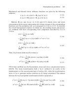
4.4. Orthogonally reinforced orthotropic layer
The simplest layer reinforced in two directions is the so-called cross-ply layer that
consists of alternating plies with 0 and 90
◦
orientations with respect to the global coordi-
nate frame x, y, and z as in Fig. 4.33. Actually, this is a laminated structure, but being
formed with a number of plies, it can be treated as a homogeneous orthotropic layer (see

Section 5.4.2).
184 Advanced mechanics of composite materials
1
2
3
x
y
z
h
1
2
3
t
yz
t
xz
t
xz
t
xy
t
yz
s
y
s
z
s
x
t
xy

Fig. 4.33. A cross-ply layer.
4.4.1. Linear elastic model
Let the layer consist of m longitudinal (0
◦
) plies with thicknesses h
(i)
0
(i = 1,
2, 3, ,m)and n transverse (90
◦
) plies with thicknesses h
(j)
90
(j = 1, 2, 3, ,n)made
from one and the same composite material. Then, stresses σ
x
, σ
y
, and τ
xy
that comprise
the plane stress state in the global coordinate frame can be expressed in terms of stresses
in the principal material coordinates of the plies as
σ
x
h =
m

i=1
σ

(i)
1
h
(i)
0
+
n

j=1
σ
(j)
2
h
(j)
90
σ
y
h =
m

i=1
σ
(i)
2
h
(i)
0
+
n


j=1
σ
(j)
1
h
(j)
90
τ
xy
h =
m

i=1
τ
(i)
12
h
(i)
0
+
n

j=1
τ
(j)
12
h
(j)
90
(4.111)

Here, h is the total thickness of the layer (see Fig. 4.33), i.e.,
h = h
0
+h
90
where
h
0
=
m

i=1
h
(i)
0
,h
90
=
n

j=1
h
(j)
90
are the total thicknesses of the longitudinal and transverse plies.
Chapter 4. Mechanics of a composite layer 185
The stresses in the principal material coordinates of the plies are related to the
corresponding strains by Eqs. (3.59) or Eqs. (4.56)
σ
(i, j )

1
= E
1

ε
(i, j )
1
+ν
12
ε
(i, j )
2

σ
(i, j )
2
= E
2

ε
(i, j )
2
+ν
21
ε
(i, j )
1

τ
(i, j )

12
= G
12
γ
(i, j )
12
(4.112)
in which, as earlier
E
1, 2
= E
1, 2
/(1 − ν
12
ν
21
) and E
1
ν
12
= E
2
ν
21
. Now assume that
the deformation of all the plies is the same as that of the deformation of the whole layer,
i.e., that
ε
(i)
1

= ε
(j)
2
= ε
x
,ε
(i)
2
= ε
(j)
1
= ε
y
,γ
(i)
12
= γ
(j)
12
= γ
xy
Then, substituting the stresses, Eqs. (4.112), into Eqs. (4.111), we arrive at the following
constitutive equations
σ
x
= A
11
ε
x
+A

12
ε
y
σ
y
= A
21
ε
x
+A
22
ε
y
τ
xy
= A
44
γ
xy
(4.113)
in which the stiffness coefficients are
A
11
= E
1
h
0
+E
2
h

90
,A
22
= E
1
h
90
+E
2
h
0
A
12
= A
21
= E
1
ν
12
= E
2
ν
21
,A
44
= G
12
(4.114)
and
h

0
=
h
0
h
,
h
90
=
h
90
h
The inverse form of Eqs. (4.113) is
ε
x
=
σ
x
E
x
−ν
xy
σ
y
E
y
,ε
y
=
σ

y
E
y
−ν
yx
σ
x
E
x
,γ
xy
=
τ
xy
G
xy
(4.115)
where
E
x
= A
11
−
A
2
12
A
22
,E
y

= A
22
−
A
2
12
A
11
,G
xy
= A
44
ν
xy
=
A
12
A
11
,ν
yx
=
A
12
A
22
(4.116)
186 Advanced mechanics of composite materials
t
xz

t
x
z
t
xz
t
xz
t
23
t
13
t
23
t
13
Fig. 4.34. Pure transverse shear of a cross-ply layer.
To determine the transverse shear moduli G
xz
and G
yz
, consider, e.g., pure shear in the
xz-plane (see Fig. 4.34). It follows from the equilibrium conditions for the plies that
τ
(i)
13
= τ
(j)
23
= τ
xz

,τ
(i)
23
= τ
(j)
13
= τ
yz
(4.117)
The total shear strains can be found as
γ
xz
=
1
h
⎛
⎝
m

i=1
γ
(i)
13
h
0
+
n

j=1
γ

(j)
23
h
90
⎞
⎠
γ
yz
=
1
h
⎛
⎝
m

i=1
γ
(i)
23
h
0
+
n

j=1
γ
(j)
13
h
90

⎞
⎠
(4.118)
where in accordance with Eqs. (4.56)
γ
(i, j )
13
=
τ
(i, j )
13
G
13
,γ
(i, j )
23
=
τ
(i, j )
23
G
23
(4.119)
Substituting Eqs. (4.119) into Eqs. (4.118) and using Eqs. (4.117), we arrive at
γ
xz
=
τ
xz
G

xz
,γ
yz
=
τ
yz
G
yz
where
1
G
xz
=
h
0
G
13
+
h
90
G
23
,
1
G
yz
=
h
0
G

23
+
h
90
G
13