The boundary element method with programming for engineers and scientists - phần 1 pps

W
/MZVW\*MMZ
1IV;UQ\P
+PZQ[\QIV,]MV[MZ
<PM*W]VLIZa
-TMUMV\5M\PWL_Q\P
8ZWOZIUUQVO
.WZMVOQVMMZ[IVL[KQMV\Q[\[
;XZQVOMZ?QMV6M_AWZS
Univ Prof. DI Dr. Gernot Beer
1V[\Q\]\MNWZ;\Z]K\]ZIT)VITa[Q[
/ZIb=VQ^MZ[Q\aWN<MKPVWTWOa)][\ZQI
8ZWN1IV5;UQ\P
=VQ^MZ[Q\aWN5IVKPM[\MZ=VQ\ML3QVOLWU
DI Dr. Christian Duenser
1V[\Q\]\MNWZ;\Z]K\]ZIT)VITa[Q[
/ZIb=VQ^MZ[Q\aWN<MKPVWTWOa)][\ZQI
<PQ[_WZSQ[[]JRMK\\WKWXaZQOP\
)TTZQOP\[IZMZM[MZ^ML_PM\PMZ\PM_PWTMWZXIZ\WN\PMUI\MZQITQ[
KWVKMZVML[XMKQâKITTa\PW[MWN\ZIV[TI\QWVZMXZQV\QVOZM][MWN
QTT][\ZI\QWV[JZWILKI[\QVOZMXZWL]K\QWVJaXPW\WKWXaQVOUIKPQVM[WZ
[QUQTIZUMIV[IVL[\WZIOMQVLI\IJIVS[
8ZWL]K\4QIJQTQ\a"<PMX]JTQ[PMZKIVOQ^MVWO]IZIV\MMNWZITT\PM
QVNWZUI\QWVKWV\IQVMLQV\PQ[JWWS<PQ[LWM[IT[WZMNMZ\WQVNWZUI\QWV
IJW]\LZ]OLW[IOMIVLIXXTQKI\QWV\PMZMWN1VM^MZaQVLQ^QL]ITKI[M\PM
ZM[XMK\Q^M][MZU][\KPMKSQ\[IKK]ZIKaJaKWV[]T\QVOW\PMZXPIZUIKM]\QKIT
TQ\MZI\]ZM<PM][MWNZMOQ[\MZMLVIUM[\ZILMUIZS[M\KQV\PQ[X]JTQKI\QWV
LWM[VW\QUXTaM^MVQV\PMIJ[MVKMWNI[XMKQâK[\I\MUMV\\PI\[]KP
VIUM[IZMM`MUX\NZWU\PMZMTM^IV\XZW\MK\Q^MTI_[IVLZMO]TI\QWV[IVL
\PMZMNWZMNZMMNWZOMVMZIT][M

 ;XZQVOMZ>MZTIO?QMV
8ZQV\MLQV/MZUIVa
;XZQVOMZ?QMV6M_AWZSQ[XIZ\WN;XZQVOMZ;KQMVKM*][QVM[[5MLQI
[XZQVOMZI\
<aXM[M\\QVO"+IUMZIZMILaJa\PMI]\PWZ[
8ZQV\QVO";\ZI][[/UJ0!!5ÕZTMVJIKP/MZUIVa
8ZQV\MLWVIKQLNZMMIVLKPTWZQVMNZMMJTMIKPMLXIXMZ
?Q\PâO]ZM[IVL\IJTM[
;816"!!
4QJZIZaWN+WVOZM[[+WV\ZWT6]UJMZ" !!
1;*6! ;XZQVOMZ?QMV6M_AWZS

Contents


Preface xiii

Acknowledgements xiv

1 Preliminaries 1

1.1 Introduction 1
1.2 Overview of book 4
1.3 Mathematical preliminaries 6
1.3.1 Vector algebra 7
1.3.2 Stress and strain 10
1.4 Conclusions 11
1.5 References 11

2 Programming 13

2.1 Strategies 13
2.2 FORTAN 90/95/2000 features 14
2.2.1 Representation of numbers 14
2.2.2 Arrays 15
2.2.3 Array operations 16
2.2.4 Control 20
2.2.5 Subroutines and functions 21
2.2.6 Subprogram libraries and common variables 23
2.3 Charts and pseudo code 24
2.4 Parallel programming 25
2.5 BLAS libraries 27
2.6 Pre- and Postprocessing 27
2.7 Conclusions 27
2.8 Exercises 28
2.9 References 29

3 Discretisation and Interpolation 31

3.1 Introduction 32
vi The Boundary Element Method with Programming
3.2 One-dimensional boundary elements 32
3.3 Two-dimesional elements 36
3.4 Three-dimensional cells 44
3.5 Elements of infinite extent 44
3.6 Subroutines for shape functions 46
3.7 Interpolation 47
3.7.1 Isoparametric elements 47
3.7.2 Infinite elements 49
3.7.3 Discontinuous elements 50

3.8 Coordinate transformation 53
3.9 Differential geometry 54
3.10 Integration over elements 59
3.10.1 Integration over boundary elements 59
3.10.2 Integration over cells 59
3.10.3 Numerical integration 60
3.11 PROGRAM 3.1: Calculation of surface area 64
3.12 Concluding remarks 65
3.13 Exercises 65
3.14 References 67

4 Material Modelling and Fundamental Solutions 69

4.1. Introduction 69
4.2. Steady state potential problems 70
4.3. Static elasticity problems 76
4.3.1 Constitutive equations 82
4.3.2 Fundamental solutions 85
4.4. Conclusions 94
4.5. References 94

5 Boundary Integral Equations 95

5.1 Introduction 95
5.2 Trefftz method 96
5.3 PROGRAM 5.1: Flow around cylinder, Trefftz method 99
5.3.1 Sample input and output 102
5.4 Direct method 104
5.4.1 Theorem of Betti and integral equations 104
5.4.2 Limiting values of integrals as P coincides with Q 107

5.4.3 Solution of integral equations 110
5.5 Computation of results inside the domain 116
5.6 PROGRAM 5.2: Flow around cylinder, direct method 118
5.6.1 Sample input and output 122
5.7 Conclusions 125
5.8 Exercises 127
5.9 References 127

CONTENTS vii
6 Boundary Element Methods – Numerical Implementation 129

6.1 Introduction 129
6.2 Discretisation with isoparametric elements 130
6.3 Integration of kernel shape function products 133
6.3.1 Singular integrals 134
6.3.2 Rigid body motion 135
6.3.3 Numerical integration 139
6.3.4 Numerical integration over one-dimensional elements 142
6.3.5 Subdivision of region of integration 146
6.3.6 Implementation for plane problems 148
6.3.7 Numerical integration for two-dimensional elements 155
6.3.8 Subdivision of region of integration 159
6.3.9 Infinite elements 160
6.3.10 Implementation for three-dimensional problems 161
6.4 Conclusions 166
6.5 Exercises 167
6.6 References 168

7 Assembly and Solution 169

7.1 Introduction 169
7.2 Assembly of system of equations 170
7.2.1 Symmetry 176
7.2.2 Subroutine MIRROR 180
7.2.3 Subroutine Assembly 183
7.3 Solution of system of equations 184
7.3.1 Gauss elimination 185
7.3.2 Scaling 187
7.4 PROGRAM 7.1: general purpose program, direct method, one region 187
7.4.1 User’s manual 195
7.4.2 Sample input file 198
7.5 Conclusions 199
7.6 Exercises 200
7.7 References 202

8 Element-by-element techniques and Parallel Programming 203

8.1 Introduction 203
8.1 The Element by Element Concept 204
8.1.1 Element-by-element storage requirements 206
8.2 PROGRAM 8.1 : Replacing direct by iterative solution 206
8.2.1 Sample input file 211
8.2.2 Sample output file 212
8.3 PROGRAM 8.2 : Replacing assembly by element-by-element procedure 213
8.3.1 Sample input file 219
8.3.2 Sample output file 219
viii The Boundary Element Method with Programming
8.4 PROGRAM 8.3 : Parallelising the element-by-element procedure 220
8.4.1 Sample input file 227
8.4.2 Sample output file 227

8.4.3 Results from larger analyses 228
8.5 Conclusions 229
8.6 References 229

9 Postprocessing 231

9.1 Introduction 231
9.2 Computation of boundary results 232
9.2.1 Potential problems 232
9.2.2 Elasticity problems 236
9.3 Computation of internal results 241
9.3.1 Potential problems 241
9.3.2 Elasticity problems 245
9.4 PROGRAM 9.1: Postprocessor 250
9.4.1 Input specification 258
9.5 Graphical display of results 259
9.6 Conclusions 261
9.7 Exercises 262
9.8 References 262

10 Test Examples 263

10.1. Introduction 263
10.2. Cantilever beam 264
10.2.1 Problem statement 264
10.2.2 Boundary element discretisation and input 264
10.2.3 Results 266
10.2.4 Comparison with FEM 269
10.2.5 Conclusions 271
10.3. Circular excavation in infinite domain 271

10.3.1 Problem statement 271
10.3.2 Boundary element discretisation and input 272
10.3.3 Results 274
10.3.4 Comparison with FEM 275
10.3.5 Conclusions 276
10.4. Square excavation in infinite elastic space 276
10.4.1 Problem statement 276
10.4.2 Boundary element discretisation and input 277
10.4.3 “Quarter point” elements 281
10.4.4 Comparison with finite elements 282
10.4.5 Conclusions 282
10.5. Spherical excavation 283
10.5.1 Problem statement 283
10.5.2 Boundary element discretisation and input 283
CONTENTS ix
10.5.3 Results 289
10.5.4 Comparison with FEM 290
10.6. Conclusions 290
10.7. References 291

11 Multiple regions 293

11.1 Introduction 293
11.2 Stiffness matrix assembly 294
11.2.1 Partially coupled problems 296
11.2.2 Example 299
11.3 Computer implementation 304
11.3.1 Subroutine Stiffness_BEM 306
11.4 Program 11.1: General purpose program, direct method, multiple regions 311
11.4.1 User’s manual 321

11.4.2 Sample problem 323
11.5 Conclusions 326
11.6 Exercises 327
11.7 References 328

12 Dealing with corners and changing geometry 329

12.1 Introduction 329
12.2 Corners and edges 330
12.2.1 Discontinuous elements 331
12.2.2 Numerical integration for one-dimensional elements 331
12.2.3 Numerical implementation 335
12.2.4 Test example – single region 343
12.2.5 Test example – multi region 344
12.3 Dealing with changing geometry 346
12.3.1 Example 348
12.4 Alternative Strategy 351
12.5 Conclusions 353
12.6 References 353

13 Body Forces 355

13.1 Introduction 355
13.2 Gravity 356
13.2.1 Post-processing 358
13.3 Internal concentrated forces 361
13.3.1 Post-processing 363
13.4 Internal distributed line forces 363
13.4.1 Post-processing 365
13.5 Initial strains 365

13.5.1 Post-processing 369
13.6 Initial stresses 372
x The Boundary Element Method with Programming
13.7 Numerical integration over cells 373
13.8 Implementation 374
13.8.1 Input data specification for Body_force 377
13.9 Sample input file and results 378
13.10 Conclusions 381
13.11 Exercises 382
13.12 References 383

14 Dynamic Analysis 385

14.1 Introduction 385
14.2 Scalar wave equation, frequency domain 385
14.2.1 Fundamental solutions 387
14.2.2 Boundary Integral Equations 388
14.2.3 Numerical Implementation 389
14.3 Scalar wave equation, time domain 390
14.3.1 Fundamental solutions 390
14.3.2 Boundary integral equations 392
14.3.3 Numerical implementation 395
14.4 Elastodynamics 398
14.4.1 Fundamental solutions 399
14.4.2 Boundary integral equations 399
14.4.3 Numerical implementation 400
14.5 Multiple regions 401
14.6 Examples 403
14.6.1 Test example 403
14.6.2 Practical application 405

14.7 References 406

15 Nonlinear Problems 407

15.1 Introduction 407
15.2 General solution procedure 408
15.3 Plasticity 410
15.3.1 Elasto-plasticity 410
15.3.2 Visco-plasticity 413
15.3.3 Method of solution 415
15.3.4 Calculation of residual {R} 417
15.3.5 Computation of stresses at cell nodes 421
15.3.6 Computation of boundary stresses 423
15.3.7 Example 425
15.4 Contact problems 427
15.4.1 Method of analysis 427
15.4.2 Solution procedure 430
15.4.3 Example of application 431
15.5 Conclusions 433
15.6 References 433
CONTENTS xi

16 Coupled Boundary Element/ Finite Element Analysis 435

16.1 Introduction 435
16.2 Coupling theory 436
16.2.1 Coupling to finite elements 436
16.2.2 Coupling to boundary elements 443
16.3 Example 444
16.4 Dynamics 446

16.4.1 Example 447
16.5 Conclusion 447
16.6 References 449

17 Industrial Applications 451

17.1 Introduction 451
17.2 Mechanical engineering 453
17.2.1 A cracked extrusion press causes concern 453
17.3 Geotechnical Engineering 457
17.3.1 CERN Caverns 457
17.4 Geological engineering 461
17.4.1 How to find gold with boundary elements 461
17.5 Civil engineering 464
17.5.1 Masjed-o-Soleiman underground power house 464
17.6 Reservoir engineering 470
17.6.1 Borehole stability 470
17.7 Conclusions 472
17.8 References 473

18 Advanced topics 475

18.1 Introduction 475
18.2 Heterogeneous Domains 476
18.2.1 Theory 476
18.2.2 Example 477
18.3 Linear inclusions 479
18.3.1 Theory 479
18.3.2 Example 484
18.4 Piezo-electricity 485

18.4.1 Changes required in General_Purpose_BEM 487
18.5 Conclusions 488
18.6 References 489

Appendix 491


xiii
Preface

This is a sequel to the book “Programming the Boundary Element Method” by G. Beer
published by Wiley in 2001. The scope of this book is different however and this is
reflected in the title. Whereas the previous book concentrated on explaining the
implementation of a limited range of problems into computer code and the emphasis was
on programming, in the current book the problems covered are extended, the emphasis is
on explaining the theory and computer code is not presented for all topics. The new topics
covered range from dynamics to piezo-electricity. However, the main idea, to provide an
explanation of the Boundary Element Method (BEM), that is easy for engineers and
scientists to follow, is retained. This is achieved by explaining some aspects of the method
in an engineering rather than mathematical way.
Another new feature of the book is that it deals with the implementation of the method
on parallel processing hardware. I. M. Smith, who has been involved in programming the
finite element method for decades, illustrates that the BEM is “embarrassingly
parallelisable”. It is shown that the conversion of the BEM programs to run efficiently on
parallel processing hardware is not too difficult and the results are very impressive, such
as solving a 20 000 element problem during a “coffee break”.
Due to the fact that, compared to the Finite Element Method, a significantly smaller
group of people are working in this field the development of the method is lagging
considerably behind. The often quoted comparison that the method is a “Cinderella”,
dominated by her “big sister”, the Finite Element Method, and whose beauty is hidden

away, is still true and we hope that the reader will see the beauty of the method in the
examples on industrial applications and the advanced topics presented at the end.
The book includes some innovative development work carried out by the small but
very active group at the Institute for Structural Analysis, Graz University of Technology,
Austria under the leadership of G. Beer. The main scope of their research is to further
develop the method, so that it can be applied to a much wider range of practical problems
in engineering, one particular application of interest being in the field of geotechnical
engineering, especially underground excavation.
COMPUTER PROGRAMS
All software (libraries and programs) can be downloaded free of charge from the website
/>



xiv
Acknowledgements

This book would not have been possible without the research effort by the small but very
active group of scientists working on boundary element methods at the Institute for
Structural Analysis, Graz University of Technology (Katherina Riederer, Andre Maues
Brabo Pereira, Klaus Thöni, Plinio Glauber Carvalho de Prazeres, Thomas Rüberg and
Jürgen Zechner). The Austrian Science Fund (FWF) and the European Commission
(under its framework program for research and technical development) contributed
significantly to the funding of the research effort.The complete set of fundamental
solutions presented in the Appendix has been supplied by Tatiana Souza Antunes Ribeiro
a former PhD student at the institute. Katherina Riederer supplied the two examples for
Chapter 18 (Advanced topics) on heterogeneous domains and linear inclusions. Andre
Periera made significant contributions to Chapter 14 (Dynamic Analysis).
The authors are grateful to Sylvia Beer for proofreading the manuscript and for her
valuable suggestions. Thanks are also due to the companies that gave the opportunity to

apply the method to the real engineering problems reported in Chapter 17: Lahmeyer
International (Bernhard Stabel), Geoconsult and Schoeller Bleckmann Austria. The
cooperation with Kuwait University (Abdullah Ebrahim) led to the application in
reservoir engineering. Last but not least our thanks go to our families for their support.



1
Preliminaries

A journey of a thousand miles
begins with a single step
Lao-tzu, Chinese philosopher
1.1 INTRODUCTION
Nearly all physical phenomena occurring in nature can be described by differential
equations and boundary conditions. In the solution of these boundary value problems
we aim to determine a response to given boundary conditions. For example we may be
interested in determining the response of the rock mass due to the excavation of a tunnel,
or the response of a structure to dynamic excitations of its foundations (caused by an
earthquake). Analytical solutions of boundary value problems, i.e. solutions that satisfy
both the differential equations (DE) and the boundary conditions (BCs), can only be
obtained for few problems with very simple boundary conditions. For example,
analytical solutions exist for the excavation of a circular tunnel in a homogeneous rock
mass, not really a realistic scenario for practical tunnelling. To be able to solve real life
problems, the engineer must revert to approximate solutions. Two approaches can be
taken: instead of satisfying both the DE and the BCs, one can attempt to satisfy only one
of the two and minimise the error in satisfying the other one. In the first approach (based
on the original idea of Ritz
1
) solutions are proposed that satisfy the boundary conditions

exactly. The error in satisfying the differential equation is then minimised. This is the
well known Finite Element Method. In the alternative (proposed by Trefftz
2
), the
assumed functions satisfy the DE exactly and the error in the satisfaction of the
boundary conditions is minimised.
Most readers of this book will be familiar with the finite element method. In the most
common version of this method we subdivide the domain into elements and approximate
2 The Boundary Element Method with Programming
the response to a specified loading with functions which are defined at element level,
i.e., are piecewise continuous. This subdivision is necessary because in practice it is
impossible to determine functions that cover the whole domain and at the same time
satisfy the boundary conditions (as originally proposed by Ritz). The parameters of these
functions, which are the values of the unknowns at the nodes where elements are
connected to each other, are determined by minimising the error in satisfying the DE.
This can be done using residual methods, where the integral of the error is minimised
and this involves a domain integral. A violation of the DE may occur at any point in the
domain, but the variation of the unknown is chosen in such a way that the error in the
satisfaction of the DE over the whole domain is a minimum. In continuum mechanics,
for example, this means that the chosen functions will usually not satisfy exactly the
equilibrium conditions at specified points.
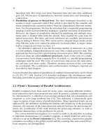
Figure 1.1 shows an example of a finite element mesh for the three-dimensional
analysis of sequential excavation and construction of a tunnel. A plane of symmetry is
applied, so that only half of the tunnel is discretised. Note that to model the rock mass
through which the tunnel is driven, which for all practical purposes can be assumed to be
infinite, we must make a 'box' of solid elements. At the outer boundaries of this box,
unless we use infinite elements, we either set displacements to zero or apply stress
boundary conditions, which represent the in situ stress. The mesh shown here has
approximately 100 000 degrees of freedom and a solution took several hours on a PC.
Note that small jumps occur in the contours of maximum compressive stress, between

elements indicating a lack of satisfaction of equilibrium locally.
The second approach to solving this problem (based on the original idea of Trefftz)
does not require the subdivision of the domain into elements because the functions used
for approximating the solution inside the domain are chosen to be those which exactly
satisfy the governing differential equations. In a similar way as with the FEM the error
in satisfying the boundary conditions is minimised and this now involves a boundary
integral. Numerically, this integral can be evaluated by subdividing the boundary into
elements over which the values (for example, tractions or displacements in the case of
continuum mechanics) are interpolated, much in the same way as with the FEM. The
advantage of the method is obvious: the dimensionality of the problem is reduced by one
order, i.e. only a surface instead of a volume integral is required. This means that the
number of unknowns is reduced dramatically, especially for three-dimensional
problems, because unknowns occur only on the problem boundary. Other advantages are
that the DE is satisfied exactly everywhere in the domain and that infinite domain
problems are easy to deal with.
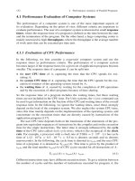
As an example, Figure 1.2 shows the boundary element mesh for the same tunnel as
analysed by the FEM in Figure 1.1. This mesh has approx. 1000 degrees of freedom and
took 3 minutes to solve on a PC. The stress contours computed and drawn on the
excavation surface and a user defined plane inside the rock mass show no jumps as they
are seen in FEM results. Since functions must be found which exactly satisfy the
governing differential equation (DE) the BEM requires a solution of the DE. This
solution must be as simple as possible because, as will be seen in the chapter on
implementation, this is crucial for efficiency. Unfortunately, the simplest solutions
which we can find (fundamental solutions) are due to concentrated loads or sources and
PRELIMINARIES 3
are singular, i.e., have infinite values at certain points. This property has to be taken into
account when integrating these functions over boundary elements. This will make the
numerical integration procedure more complicated than is the case with finite elements.

Figure 1.1 Finite element mesh for the analysis of tunnel excavation. Left side: mesh

with contours of z-displacement; right side: detail with contours of
maximum compressive stress
Figure 1.2 Boundary element mesh for the simulation of tunnel excavation with
contours of maximum compressive stress plotted

on excavation surface
and result planes
4 The Boundary Element Method with Programming

There has been a general misconception that because a fundamental solution of the
problem must exist for the BEM to work, the method can only be applied to linear
problems with homogeneous material. As will be shown in this book, non-linear
problems can almost as easily be solved as with the FEM, by the repeated solution of
linear problems and special methods may be employed to solve problems with
heterogeneous material properties.
1.2 OVERVIEW OF BOOK
This book is designed to be used as basis for a course on the BEM or for self study.
It is recommended that chapters be read consecutively as later chapters build on material
discussed earlier. Throughout the book, the reader will build a suite of subprograms,
which perform the various tasks needed for the numerical implementation of the BEM.
Various exercises are included which allow the reader to test the programs written and
experience how the method works.
We start with an introduction to the FORTRAN 95 programming language.
FORTRAN, which stands for FORMula TRANslation is still the most widely used
language for programming engineering applications and is easier to learn and more
efficient than other high level languages such as C++. However, there is no reason why
the procedures outlined in some detail in this book could not be implemented in another
language.
The next chapter deals with the way in which we can describe the geometrical
boundary of a problem and boundary conditions in a numerical way. This is done by

subdividing the surface into small elements and by interpolating between nodal values.
This is essential for the later treatment of integral equations. With the aid of the
examples we can not only test the subroutines developed but also get an understanding
of the error introduced by the approximations used to describe boundaries.
Another fundamental building block is the description of the material response. In
Chapter 4 we introduce basic concepts of elasticity and potential flow and develop
fundamental solutions, that is, simple solutions which satisfy the governing differential
equations. These will be central to our subsequent deliberations.
Next we introduce the concepts of boundary element methods using the method
originally proposed by Trefftz. Although this very simple method cannot be used for
general purpose programs, it serves very well to explain the fundamental ideas of the
method. A small computer program can be developed to solve some simple problems.
Again, this will serve as a tool for learning by experience.
The direct boundary element method used in the majority of BEM software is
introduced next. Here we will use the reciprocal theorem by Betti, which is well known
to engineers to obtain an integral equation. The major task in the implementation
however, is to solve the integral equations numerically.
The next chapter on numerical implementation therefore deals with the evaluation of
integrals using numerical integration. Those familiar with isoparametric finite elements
will recognise the Guass Quadrature method used. However, in contrast to its use in the
PRELIMINARIES 5
FEM, one must be very careful to select the number of integration points, as they are
dependent on how close the singularity is to the integration region. This is the most
difficult and crucial part in the implementation of the BEM. The integration over the
boundary surface is carried out over a boundary element and the contributions of all
elements which describe a boundary are then added. We will see that this is very similar
to the assembly procedure in the FEM.
After the numerical treatment of the integral equations we end up with a system of
equations. In contrast to the FEM, the coefficient matrix is fully populated and
unsymmetrical. Standard Gauss elimination can be used but, for large systems, the

storage requirement and the computation times may be reduced considerably by iterative
solvers, such as conjugate gradient methods. Such special solution techniques are
introduced in the next chapter. Here we also find that the method is “embarrassingly
parallelisable” i.e. that excellent speed up rates can be achieved with special hardware.
The primary results obtained from the analysis are values of displacement or traction
at the boundary depending on the boundary condition specified. In contrast to the FEM,
primary results do not include values in the interior of the domain but these are
computed by post-processing. In Chapter 9 it is explained how the stresses at the
boundary and in the interior can be obtained from boundary displacements and tractions.
This is indeed an advantage of the method, because the user has free choice of the
locations where results are obtained.
We now have all the building blocks together and are able to compile a computer
program that is able to solve two and three-dimensional problems in elasticity and
potential flow, depending on which fundamental solution is used. In Chapter 10 we
apply the program developed to test examples and find out what level of accuracy can be
obtained in comparison with the FEM.
For inhomogeneous domains, where we can not obtain a fundamental solution, we
introduce the concept of multiple regions, where the domain is subdivided into sub-
regions, similar to the FEM. There is an additional advantage in this concept, because
sparseness is introduced in the system of equations. We will also find out in a later
chapter that the multi-region method allows contact and excavation problems to be
solved in an elegant way.
In the next chapter we deal with problems that involve corners and geometry which
changes with time, as is the application to sequential excavation/construction of a tunnel.
Because elements only exist on the boundary the BEM has difficulty dealing with
problems where forces are applied inside the domain. These forces can be loosely
termed “body forces”. It will be shown that an additional volume integral has to be
considered. For body forces that are constant the volume integral can be transformed
into a surface integral. However, if the body forces are not constant throughout the
domain the volume integral needs to be evaluated numerically. This can be done by

using internal cells, which look like finite elements, but do not involve any additional
degrees of freedom, as they are only used for integration. The implementation of this
procedure, discussed in chapter 13 also allows the solution of problems in elasto- and
visco-plasticity. Body forces of a different kind (mass forces) occur in the case of
dynamics, but their treatment with the BEM is quite different to the FEM and this is
discussed in Chapter 14.
6 The Boundary Element Method with Programming
In Chapter 15 we show that the solution of non-linear problems follows similar
procedures as in the FEM and that the general solution algorithm is similar. Here two
types of non-linear problems are discussed in more detail: plasticity and contact
problems.
It is possible to couple the BEM with the FEM thus getting the ‘best of both worlds’.
In Chapter 16, methods of coupling are presented. Basically, a stiffness matrix of the BE
region is obtained and assembled with the FEM stiffness matrices. Since many general
purpose programs allow the input of a user defined element stiffness matrix this may be
used to extend the capabilities of a reader’s FEM code.
To demonstrate that the method also works for large scale industrial problems,
Chapter 17 shows some applications of the boundary and coupled method in
engineering. The purpose of this chapter is twofold: firstly it shows how complex
problems, as they invariably occur in real life, can be simplified and how a suitable
boundary element mesh is obtained. Secondly it shows the advantage of the BEM and
the coupled BEM/FEM in terms of user friendliness and computing time.
The last chapter deals with topics which were still subject to research at the writing
of the book. The first deals with the efficient treatment of heterogeneous ground
conditions the other with the consideration of linear inclusions such as reinforcement
and rock bolts. The application in piezo-electricity shows the flexibility of the method to
deal with any problem whose fundamental solution is known.
By the end of this book the reader should have an understanding of how the method
works, of its potential and how it can be implemented into a computer program.
1.3 MATHEMATICAL PRELIMINARIES

A good consistent notation is essential to any textbook. For the development and
explanation of numerical methods two notations are used by engineers: matrix and
tensor notation. Traditionally, textbooks on the BEM have use tensor notation, whereas
those about the FEM have used matrices, although this is rapidly changing. The main
notation chosen for this book is the matrix notation.
There are two reasons for this: firstly, the book which is probably still the most
widely read on numerical modelling, “The Finite Element Method”, by O.C.
Zienkiewicz and R.L Taylor
3
, uses matrix notation throughout. Since we hope to attract
more engineers to the BEM, this was one motivation. The other reason is that books on
the BEM that use tensor notation have to revert to matrix notation at some stage, for
example when discussing the assembly of the system of equations. Thus the book
attempts to avoid two different notations.
However, when discussing fundamental solutions and their derivatives it transpires
that tensor notation is much easier to use. Therefore in this book we have made a
compromise in that for this case only we revert to a simplified version of the tensor
notation.
In the following we discuss some basic mathematics which will be used in this book
and also attempt a comparison of matrix and tensor notation.

PRELIMINARIES 7
1.3.1 Vector algebra

Vectors are used to represent a displacement/force or to define the position of a point
relative to a set of Cartesian axes. We define the position of a point in 3-D space with
respect to Cartesian axes x, y, z (Figure 1.3) as


(2.1)

Figure 1.3 Position vector x defining a point in space
Alternatively, we may represent the point in terms of Cartesian coordinates x
i
, where
i=1,2,3 (the last number is also referred to as range).
The components are specified with respect to a set of orthogonal coordinate axes,
which are defined by base vectors of unit length, i
i
and which have the property:

(2.2)
where
 
x
denotes the scalar (dot) product
(2.3)
and
G
ij
is known as the Kronecker delta.
Vector x may then be represented in indicial notation as
(2.4)
°
¿
°
¾
½
°
¯
°

®

z

x
ji
ji
ijji
for 0
for 1
G
ii
ii
i
ii
xx iix
¦

3
1
x
x
y
z
1
i
2
i
3
i

°
°
¿
°
°
¾
½
°
°
¯
°
°
®


z
y
x
x
12 12 12ij xx yy zz
ii ii iix   ii
8 The Boundary Element Method with Programming
where the Einstein summation convention has been used for the last term. This
convention specifies that for any index which is repeated and which does not appear on
the left hand side, a summation of all terms within the
range is implied.
Another vector quantity is the displacement which can be written either as
(2.5)

in matrix notation or

ii
u ui in indicial notation
Coordinate transformation
If we want to express the location of a point, x in another orthogonal coordinate system
(
x ) the directions of which are given by unit vectors v
1
, v
2
, v
3
then in matrix notation
we write
(2.6)

where the transformation matrix is defined as
(2.7)

Alternatively, we may write in indicial notation
(2.8)

where
(2.9)

Projection of one vector onto another

If we want to compute the projection of a vector onto a direction specified by a unit
vector
v, then it is very convenient to use the dot product. For example, the component,
u

c
of the displacement u in the direction specified by v is given by
(2.10)

The angle
T
between the two vectors is computed by
(2.11)

g
xTx
>@
321
vvvT
g
iijj
x
x /
jiij
iv
x
/

x
y
z
u
u
u
½

°°

®¾
°°
¯¿
u
vux
c
u
vu
u
x
1
T
cos
PRELIMINARIES 9

where the length of vector
u is given by
(2.12)

Figure 1.4
Projection of vector
Derivatives of vectors
The derivatives of the displacement vector may be written as
(2.13)


In indicial notation we simply write
(2.14)

u
v

u
c
T
,,,
;;
x
x
x
yyy
xyz
zz
z
u
uu
y
x
z
uuu
x
xy yz z
uu
u
x
z
y
w

½
ww
½ ½
°°
°° °°
w
ww
°°
°° °°
°°
www
°° °°
www
°°

®¾ ®¾ ®¾
wwwwww
°° °° °°
ww°° °° °°
w
°° °° °°
ww
w
¯¿ ¯¿
°°
¯¿
uuu
uuu
j,i
j

i
u
x
u

w
w
222
zyx
uuu  u
10 The Boundary Element Method with Programming
1.3.2 Stress and strain
Stresses and strains are tensorial quantities. In the indicial notation the strain tensor is
defined by
(2.15)

In this book, however, we use a notation originally proposed by Timoshenko
4
.
We define a
pseudo-vector of strain, i.e., a matrix with one column:
(2.16)

Note that in the pseudo-vector notation we only have 6 strain components, whereas
the symmetric strain tensor has 9. Also note that the ½ term is missing for the shear
strains in order to achieve consistency between the tensor and matrix operations. The
index number of the location of the strain or stress components for matrix notation and
tensor notation is given in Table 1.1

Table 1.1 Index numbering for strain and stress

Notation Index number
Matrix 1 2 3 4 5 6
Tensor 11
xx
22
yy
33
zz
12&21
xy&yx
23&32
yz&zy
31&13
zx&xz

Similarly, the stress tensor
ij
V
can be written as a pseudo-vector
(2.17)


i,jj,iij
uu 
2
1
H
°
°

°
°
°
°
°
¿
°
°
°
°
°
°
°
¾
½
°
°
°
°
°
°
°
¯
°
°
°
°
°
°
°

®

w
w

w
w
w
w

w
w
w
w

w
w
w
w
w
w
w
w

°
°
°
¿
°
°

°
¾
½
°
°
°
¯
°
°
°
®


x
u
z
u
y
u
z
u
x
u
y
u
z
u
y
u
x

u
z
x
z
y
y
x
z
y
x
xz
yz
xy
z
y
x
J
J
J
H
H
H
H
>@
T
xzyzxyzyx
WWWVVV

V
PRELIMINARIES 11

1.4 CONCLUSIONS
At the beginning of this chapter we have shown on an example in geomechanics that
substantial gains can be made with the BEM, in terms of mesh generation and solution
times. These gains are most pronounced for problems involving infinite or semi-infinite
domains. Other examples where the BEM seems to be superior to the FEM is for
problems where boundary stresses are important, e.g. in Mechanical Engineering.
Examples of this will be shown later.
The main purpose of this book is to encourage the use of the method. The simple
computer programs included contain all the necessary building blocks for building more
advanced and more specific computer programs for research or industrial applications.
In conclusion the reader should see this book as an advanced introduction to the
BEM, with some basic building blocks for computer programming.
1.5 REFERENCES

1. Ritz, W. (1909) Über eine Methode zur Lösung gewisser Variations-Probleme der
mathematischen Physik.
Journal für reine und angewandte Mathematik, 135:1-61.
2. Trefftz, E. (1926) Ein Gegenstück zum Ritz’schen Verfahren. Proc. 2
nd
int. Congress
in Applied Mechanics, Zurich, pp 131.
3. Zienkiewicz O.C. and Taylor R.L. (2000) The Finite Element Method - Fifth Edition.
Butterworth-Heinemann, UK.
4. Timoshenko, S.P. and Goodier, J.N. (1970) Theory of Elasticity.
McGraw-Hill,
London.
2
Programming
Art is only pleasing if it
has the character of lightness

J.W. von Goethe

2.1 STRATEGIES
Although the first idea which provided the background for the boundary element method
dates back to the early 1900s, the method only emerged when digital computers became
available. This is because, except for the simplest problems, the number of computations
required is too large for ‘hand calculation’.
The implementation into a computer application basically consists of giving the
processor a series of instructions, or tasks, to perform. In the early days these
instructions had to be given in complicated machine code and writing them was mainly
the domain of specialised programmers. Very soon higher level languages were
developed which made the programming task easier and this had the additional
advantage that code developed could run on any hardware. One of these languages,
especially developed for scientists and engineers, was FORTRAN. In the past decades,
the language has undergone tremendous development. Whereas with FORTRAN IV the
writing of programs was rather lengthy and tedious and the code difficult to follow, the
new facilities of FORTRAN 90/95/2000 (F90) make it suitable for writing short,
readable code. This has mainly to do with features that do away with the need to use
statement numbers and the availability of powerful array and matrix manipulation tools.
Today, any engineer should be able to write a program in a rather short time.
When developing a relatively large program, such as will be attempted in this book, it
is important to use the concept of modular programming. This means that the task has to