The boundary element method with programming for engineers and scientists - phần 2 pptx
Bạn đang xem bản rút gọn của tài liệu. Xem và tải ngay bản đầy đủ của tài liệu tại đây (491.05 KB, 50 trang )
40 The Boundary Element Method with Programming
If the element shape functions for the quadratic element are derived from Lagrange
polynomials, then there is an additional node at the centre of the element (Figure 3.10).
The shape functions are given by
(3.19)
Figure 3.11 Serendipity and Lagrange shape functions
321321, jjjiiijin
BBBAAAL
1
1
1
1
1
DISCRETISATION AND INTERPOLATION 41
A
i,l
is defined in equation (3.12) and
(3.20)
where
i and j are the column and row numbers of the nodes. This numbering is defined
in Figure 3.10. The nodes are given by
n (1,1) = 1 n (2,1) = 2 n (3,1) = 5
n (1,2) = 4 n (2,2) = 3 n (3,2) = 7
n (1,3) = 8 n (2,3) = 6 n (3,3) = 9
The Serendipity and Lagrange shape functions are compared in Figure 3.11
The Lagrange element has an additional ‘bubble mode’ and is, therefore, able to describe
complicated shapes more accurately. Triangular elements can be formed from
quadrilateral elements, by assigning the same global node number to two or three corner
nodes. Such degenerate elements are shown in Figure 3.12.
Figure 3.12 Linear and quadratic degenerate elements
Alternatively triangular elements may be defined using the iso-parametric concept. In
Figure 3.13 we show a triangular element in the global and local coordinate system. The
shape functions for the transformation are defined as
4
(3.21)
1
m
jm
jm
jm
Bifjm
Bifjm
KK
KK
z
8
1
374
6
2
5
ȟ
Ș
2
34
1
Ș
ȟ
1
2
3
(,) 1
(,)
(,)
N
N
N
[
K[K
[K [
[K K
42 The Boundary Element Method with Programming
Figure 3.13 Triangular linear element in global and local coordinate system
As can be seen in Figure 3.14 the shape functions are represented by planes.
Figure 3.14 Shape functions of linear triangular boundary element
It is also possible to define a triangular element with a quadratic shape function. The
shape functions for the mid-side nodes are given by
(3.22)
3
1
2
ȟ
Ș
11
(ȟ 0, Ș 0)
22
(ȟ 1, Ș 0)
33
(ȟ 0, Ș 1)
x
z
y
1
2
3
ȟ
4
5
6
41
4
41
N
N
N
[[K
[K
K[K
DISCRETISATION AND INTERPOLATION 43
The corner node functions are constructed in a similar way as for the previous
elements
(3.23)
Figure 3.15 Triangular quadratic element
3.4 THREE-DIMENSIONAL CELLS
For the description of cells for 3-D problems three-dimensional elements are used.
Their derivation is analogous to that of the two-dimensional elements described
previously, except that now three intrinsic coordinates (
[
,
K
,
]
) are used, as shown in
Figure 3.16. The Cartesian coordinates of a point with intrinsic coordinates (
[
,
K
,
]
) are
obtained by
(3.24)
Bilinear shape functions are used for the quadrilateral element in Figure 3.16
(12.1)
146
245
356
11
1
22
11
22
11
22
NNN
NNN
NNN
[K
[
K
1
2
3
4
5
6
0
[
1
2
[
1
[
1
K
1
2
K
[
K
8
1
,,
e
nn
n
N
[K]
¦
xx
]]KK[[
nnnn
N 111
8
1
44 The Boundary Element Method with Programming
where local coordinates of the nodes are defined in Table 3.2. For the description of cells
with a quadratic shape function, see for example [4].
Figure 3.16 3-D cell element in a) global and b) local coordinate system
Table 3.2 Local coordinates of nodes for 3-D cells
n
n
[
n
K
n
]
n
n
[
n
K
n
]
1 -1.0 -1.0 1.0 5 -1.0 -1.0 -1.0
2 1.0 -1.0 1.0 6 1.0 -1.0 -1.0
3 1.0 1.0 1.0 7 1.0 1.0 -1.0
4 -1.0 1.0 1.0 8 -1.0 1.0 -1.0
3.5 ELEMENTS OF INFINITE EXTENT
It is sometimes necessary to describe surfaces of infinite extent. Examples are found in
geomechanics, where either the surface of the ground extends to infinity or a tunnel can
be assumed to be infinitely long. To describe the geometry of an element of infinite
extent in one intrinsic coordinate direction, we may use special shape functions
5
which
tend to infinity, as the intrinsic coordinate tends to +1. For the one-dimensional element
shown in Figure 3.17 the coordinate transformation
(3.25)
e
n
n
n
N xx )()(
3
1
[ [
¦
f
Ș
4
1
2
ȟ
3
ȟ
Ș
x
z
a)
b
)
y
]
]
5
6
7
8
DISCRETISATION AND INTERPOLATION 45
results in infinite Cartesian coordinates at
[
= 1 if the shape functions are taken to vary
as follows:
(3.26)
Figure 3.17 One-dimensional infinite element in a) global and b) local coordinate space
Note that the element is finite in the local coordinate space and therefore can be treated
the same way as a finite boundary element for the integration.
Figure 3.18 Two-dimensional infinite element in a) global and b) local coordinate space.
The concept can be extended to two-dimensions. The geometry of the two-
dimensional element shown in Figure 3.18, for example, is described by
12
2 /(1 ) and ( 1) /(1 ) NN
[[ [ [
ff
[
x
y
[
[
[
[
a)
b)
1
2
a)
1 at infinity
[
Ș
4
1
2
ȟ
3
ȟ
Ș
x
z
a)
b
)
y
=1 at infinity
K
5
6
46 The Boundary Element Method with Programming
(3.27)
where
()
()
mn
N
[
are linear or quadratic Serendipity shape functions as presented for the
one-dimensional finite boundary elements,
()
()
kn
N
K
f
are the same infinite shape
functions as for the one-dimensional element, with
K
substituted for
[
and the values
for
m(n) and k(n) are given in Table 3.3
Table 3.3 Values for m and k in Equation (3.27)
n m
k
1 1 1
2 2 1
3 2 2
4 1 2
5 3 1
6 3 2
3.6 SUBROUTINES FOR SHAPE FUNCTIONS
Here we start building our library of Subroutines for future use. We create routines for
the calculation of Serendipity, infinite and Lagrange shape functions. Only the listing for
the first one is shown here.
As explained in Chapter 3, some variables will be defined as global, that is, as
accessible to all the subroutines in a MODULE and all programs which use them via the
USE statement. The dimensions for the array Ni, which contains the shape functions,
depend on the type of element and will be set by the main program.
SUBROUTINE Serendip_func(Ni,xsi,eta,ldim,nodes,inci)
!
! Computes Serendipity shape functions Ni(xsi,eta)
! for one and two-dimensional (linear/parabolic) finite
! boundary elements
!
REAL,INTENT(OUT) :: Ni(:) ! Array with shape function
REAL,INTENT(IN) :: xsi,eta! intrinsic coordinates
INTEGER,INTENT(IN):: ldim ! element dimension
INTEGER,INTENT(IN):: nodes ! number of nodes
INTEGER,INTENT(IN):: inci(:)! element incidences
REAL:: mxs,pxs,met,pet ! temporary variables
SELECT CASE (ldim)
CASE(1)! one-dimensional element
4(6)
() ()
1
e
mn kn n
n
NN
[K
f
¦
xx
DISCRETISATION AND INTERPOLATION 47
Ni(1)= 0.5*(1.0 - xsi); Ni(2)= 0.5*(1.0 + xsi)
IF(nodes == 2) RETURN! linear element finished
Ni(3)= 1.0 - xsi*xsi
Ni(1)= Ni(1) - 0.5*Ni(3); Ni(2)= Ni(2) 0.5*Ni(3)
CASE(2)! two-dimensional element
mxs=1.0-xsi; pxs=1.0+xsi; met=1.0-eta; pet=1.0+eta
Ni(1)= 0.25*mxs*met ; Ni(2)= 0.25*pxs*met
Ni(3)= 0.25*pxs*pet ; Ni(4)= 0.25*mxs*pet
IF(nodes == 4) RETURN! linear element finished
IF(Inci(5) > 0) THEN !zero node = node missing
Ni(5)= 0.5*(1.0 -xsi*xsi)*metNi(1)= Ni(1) - 0.5*Ni(5) ;
Ni(2)= Ni(2)0.5*Ni(5)
END IF
IF(Inci(6) > 0) THEN
Ni(6)= 0.5*(1.0 -eta*eta)*pxs
Ni(2)= Ni(2) - 0.5*Ni(6) ; Ni(3)= Ni(3) - 0.5*Ni(6)
END IF
IF(Inci(7) > 0) THEN
Ni(7)= 0.5*(1.0 -xsi*xsi)*pet
Ni(3)= Ni(3) - 0.5*Ni(7) ; Ni(4)= Ni(4)- 0.5*Ni(7)
END IF
IF(Inci(8) > 0) THEN
Ni(8)= 0.5*(1.0 -eta*eta)*mxs
Ni(4)= Ni(4) - 0.5*Ni(8) ; Ni(1)= Ni(1) - 0.5*Ni(8)
END IF
CASE DEFAULT ! error message
CALL Error_message('Element dimension not 1 or 2')
END SELECT
RETURN
END SUBROUTINE Serendip_func
3.7 INTERPOLATION
In addition to defining the shape of the solid to be modelled, we will also need to specify
the variation of physical quantities (displacement, temperature, traction, etc.) in an
element. These can be interpolated from the values at the nodal points.
3.7.1 Isoparametric elements
The value of a quantity q at a point inside an element e can be written as
(3.28)
where
e
n
q is the value of the quantity at the nth node of element e and
n
N
are
interpolation functions (Figure 3.19).
e
nn
qNq
¦
48 The Boundary Element Method with Programming
If for a particular element the same functions are used for the element shape and for the
interpolations of physical quantities inside the element, then the element is called
‘isoparametric’ (i.e., same number of parameters).
Figure 3.19 Variation of q along a quadratic 1-D boundary element (in local coordinate system)
Figure 3.20 Interpolation of q over a linear 2-D element
The variation of physical quantities on the surface of two-dimensional elements or
inside plane elements can be described (Figure 3.20)
(3.29)
Note than
q may be a scalar or a vector (i.e. may refer to tractions t or displacements
u). The physical quantities are defined for each element separately, so they can be
discontinuous at nodes shared by two elements as shown in Figure 3.21. If Serendipity
or Lagrange shape functions are used only
C
0
continuity can be enforced between
elements by specifying the same function value for each element at a shared node.
,,
e
nn
qNq
[K [K
¦
(,)q
[K
[
K
1
2
3
4
1
e
q
2
e
q
3
e
q
4
e
q
[
[
[
[
1
2
3
1
e
q
3
e
q
2
e
q
()q
[
DISCRETISATION AND INTERPOLATION 49
Figure 3.21 Variation of q with discontinuous variation at common element nodes
3.7.2 Infinite elements
For the one-dimensional infinite element we can assume that the displacements and
tractions decay from node 1 to infinity with
o(1/r) and o(1/r
2
) respectively, or that they
remain constant. The former corresponds to a surface that extends to infinity, but the
loading is finite, the latter corresponds to a the case where both the surface and the
loading extends to infinity (this corresponds to
plane strain conditions). For the one-
dimensional “decay” infinite element we have
(3.30)
where
(3.31)
For the “plane strain” infinite element the variation is given simply by
(3.32)
For the two-dimensional “decay” infinite element we have
(3.33)
1
2
3
1
1
q
1
3
q
1
2
q
()q
[
1
2
3
2
1
q
2
3
q
2
2
q
()q
[
Element 1
Element 2
11 11
;
ut
NN
ff
uutt
2
11
11
(1 ) ; (1 )
24
ut
NN
[
[
ff
2(3) 2(3)
11
11
;
ee
nu n ntn
nn
NN NN
[K [K
ff
¦¦
uutt
11
; uu tt
50 The Boundary Element Method with Programming
Where
()
n
N
[
are linear or quadratic Serendipity shape functions as presented for the
one-dimensional finite boundary elements and
1
()
t
N
K
f
and
1
()
u
N
K
f
are the same infinite
shape functions as for the one-dimensional element with
K
substituted for
[
.
For the two-dimensional “plane strain” infinite element we have
(3.34)
3.7.3 Discontinuous elements
Later we will see that in some cases it is convenient to interpolate q not from the nodes
that define the geometry but from other (interpolation) nodes that are moved inside the
element.
Figure 3.22 One dimensional linear discontinuous element
This type of element will be used in the Chapter on corners and edges to avoid a
multiple definition of the traction vector. For the one-dimensional linear element in
Figure 3.22 we have
(3.35)
Where
e
n
q are the values of q at the interpolation nodes and the interpolation functions
are
(3.36)
112 2
12 12
11
() ( ) ; () ( )
() ()
NdN d
dd dd
[
[[ [
() ()
e
nn
qNq
[[
¦
2(3) 2(3)
11
;
ee
nn nn
nn
NN
[[
¦¦
uutt
[
1
e
q
2
e
q
geometric node
interpolation node
1
d
2
d
1
2
()q
[
DISCRETISATION AND INTERPOLATION 51
Here d
1
, d
2
are absolute values of the intrinsic coordinate of the interpolation nodes.
Figure 3.23 One dimensional quadratic discontinuous element
It can be easily verified that for d
1
=d
2
=1 the shape functions for the continuous element
are obtained. For a quadratic element we have
(3.37)
Figure 3.24 Two-dimensional linear discontinuous element
For the two-dimensional linear element shown in Figure 3.24 the shape functions are
given for the corner nodes by
(3.38)
11 2 2
12 2 12 1
312
12
11
() ( )(1 ) ; () ( )(1 )
() ()
1
() ( )( )
NdNd
dd d dd d
Ndd
dd
[
[
[[[[
[[[
1132 23
324414
1234
11
(,) ( )( ) ; (,) ( )( )
11
(,) ( )( ) ; (,) ( )( )
()()
NddN dd
cc
NddNdd
cc
cdddd
[
K[K[K[K
[
K[K[K[K
(,)q
[K
[
K
1
2
3
4
1
e
q
2
e
q
3
e
q
4
e
q
d
2
d
1
d
3
d
4
1
2
3
4
[
1
e
q
2
e
q
3
e
q
1
d
2
d
1
2
3
()q
[
52 The Boundary Element Method with Programming
Figure 3.25 Two-dimensional quadratic discontinuous element
For the quadratic element in Figure 3.25 we have for the corner nodes
(3.39)
and for the mid side nodes:
(3.40)
5123
12 3 4
6234
34 1 2
7124
12 3 4
8134
34 1 2
1
(,) ( )( )( )
()
1
( , ) ( )( )( )
()
1
( , ) ( )( )( )
()
1
( , ) ( )( )( )
()
Nddd
dd d d
Nddd
dd d d
Nddd
dd d d
Nddd
dd d d
[
K[[K
[
K[[K
[
K[[K
[
K[[K
113
1234 2 4
223
1234 1 4
324
1234 1 3
414
1234 2 3
1
(,) ( )( )(1 )
()()
1
(,) ( )( )(1 )
()()
1
(,) ( )( )(1 )
()()
1
( , ) ( )( )( 1 )
()()
Ndd
dddd d d
Ndd
dddd d d
Ndd
dddd d d
Ndd
dddd d d
[
K
[K [ K
[
K
[K [ K
[
K
[K [ K
[
K
[K [ K
(,)q
[K
[
K
1
e
q
2
e
q
3
e
q
4
e
q
d
1
d
2
d
3
d
4
1
2
3
4
5
6
7
8
5
e
q
6
e
q
7
e
q
8
e
q
DISCRETISATION AND INTERPOLATION 53
3.8 COORDINATE TRANSFORMATION
Sometimes it might be convenient to define the coordinates of a node in a local
Cartesian coordinate system. A local coordinate system is defined by the location of its
origin,
x
0
and the direction of the axes. In two dimensions we define the direction with
two vectorsas shown in Figure 3.26a. The global coordinates of a point specified in a
local coordinates system
x are given by
(3.41)
where
x
0
is a vector describing the position of the origin of the local axes. For two-
dimensional problems the geometric transformation matrix is given by
(3.42)
where
12
,vvare orthogonal unit vectors specifying the directions of ,
x
y .
For three-dimensional problems a local (orthogonal) coordinate system is defined by
unit vectors
123
,,vv vas shown in Figure 3.26b. The transformation matrix for a 3-D
coordinate system is given by
(3.43)
The inverse relationship between local and global coordinates is given by
(3.44)
Figure 3.26 Local coordinate systems a) 2-D and b) 3-D
0
g
xx Tx
12
12
x
x
g
yy
vv
vv
ªº
«»
«»
¬¼
T
»
»
»
»
¼
º
«
«
«
«
¬
ª
zzz
yyy
xxx
g
vvv
vvv
vvv
321
321
321
T
0
T
g
xx Tx
x
y
x
y
0
x
1
v
2
v
x
y
x
y
0
x
2
v
1
v
z
z
3
v
)a
)b
54 The Boundary Element Method with Programming
3.9 DIFFERENTIAL GEOMETRY
In the boundary element method it will be necessary to work out the direction normal to
a line or surface element.
Figure 3.27 Vectors normal and tangential to a one-dimensional element
The best way to determine these directions is by using vector algebra. Consider a
one-dimensional quadratic boundary element (Figure 3.27). A vector in the direction of
[
can be obtained by
(3.45)
By the differentiation of equation (3.4) we get
(3.46)
A vector normal to the line element,
V
3
, may then be computed by taking the cross-
product of
V
[
with a unit vector in the z-direction (v
z
):
(3.47)
This vector product can be written as:
(3.48)
3
1
e
n
n
n
N
[
[[
w
w
ww
¦
Vx x
z
vVV u
[
3
°
°
°
¿
°
°
°
¾
½
°
°
°
¯
°
°
°
®
°
¿
°
¾
½
°
¯
°
®
u
°
°
°
¿
°
°
°
¾
½
°
°
°
¯
°
°
°
®
°
¿
°
¾
½
°
¯
°
®
0
1
0
0
3
3
3
3
[
[
[
[
[
d
dx
d
dy
d
dz
d
dy
d
dx
V
V
V
z
y
x
V
xV
[w
w
[
[
[
V
3
v
DISCRETISATION AND INTERPOLATION 55
The length of the vector V
3
is equal to
(3.49)
and therefore the unit vector in the direction normal to a line element is given by
(3.50)
It can be shown that the length of
V
3
represents also the real length of a unit segment
(
1
[
'
) in local coordinate space (this is also known as the Jacobian J of the
transformation from local to global coordinate space).
Figure 3.28 Computation of normal vector for two-dimensional elements
For two-dimensional surface elements (Figure 3.28), there are two tangential vectors,
V
[
in the
[
-direction and
(3.51)
in the
K
-direction, where
(3.52)
The vector normal to the surface may be computed by taking the cross-product of
V
[
and
V
K
:
33
3
1
V
vV
K
K
w
w
Vx
e
n
n
N
xx
¦
w
w
w
w
KK
22
33
V
dy dx
J
dd
[[
V
56 The Boundary Element Method with Programming
(3.53)
that is
(3.54)
As indicated previously the unit normal vector
v
3
is obtained by first computing the
length of the vector:
(3.55)
This is also the real area of a segment of size 1x1 in the local coordinate system, or the
Jacobian of the transformation. The normalised vector in the direction perpendicular to
the surface of the element is given by
(3.56)
It should be noted here that
,
[
K
vvare not orthogonal to each other. An orthogonal
system of axes is required for the definition of strains and stresses needed later. Here we
assume that the first axis defined by vector
v
1
is in the direction of v
[
. The second axis is
defined by:
(3.57)
The computation of the normal vector requires the derivatives of the shape functions.
These are computed by SUBROUTINE Serendip_deriv shown below.
SUBROUTINE Serendip_deriv(DNi,xsi,eta,ldim,nodes,inci)
!
! Computes Derivatives of Serendipity shape functions
! for one and two-dimensional (linear/parabolic)
! finite boundary elements
!
REAL,INTENT(OUT) :: DNi(:,:) ! Derivatives of Ni
REAL, INTENT(IN) :: xsi,eta ! intrinsic coordinates
INTEGER,INTENT(IN):: ldim ! element dimension
INTEGER,INTENT(IN):: nodes ! number of nodes
INTEGER,INTENT(IN):: inci(:) ! element incidences
K[
VVV u
3
222
3333xyz
VVVVJ
3
33
1
V
Vv
3
x
xyzyz
y y zx zx
zz xyxy
[
K[KK[
[
K[KK[
[
K[KK[
½½ ½
w w ww ww
°°°°° °
ww wwww
°°°°° °
°°°°° °
w w ww ww
u
®¾®¾® ¾
ww wwww
°°°°° °
°°°°° °
ww wwww
°°°°° °
ww wwww
¯¿¯¿¯ ¿
V
213
uvvv
DISCRETISATION AND INTERPOLATION 57
REAL:: mxs,pxs,met,pet ! temporary variables
SELECT CASE (ldim)
CASE(1) ! one-dimensional element
DNi(1,1)= -0.5
DNi(2,1)= 0.5
IF(nodes == 2)RETURN ! linear element finished
DNi(3,1)= -2.0*xsi
DNi(1,1)= DNi(1,1) - 0.5*DNi(3,1)
DNi(2,1)= DNi(2,1) - 0.5*DNi(3,1)
CASE(2) ! two-dimensional element
mxs= 1.0-xsi
pxs= 1.0+xsi
met= 1.0-eta
pet= 1.0+eta
DNi(1,1)= -0.25*met
DNi(1,2)= -0.25*mxs
DNi(2,1)= 0.25*met
DNi(2,2)= -0.25*pxs
DNi(3,1)= 0.25*pet
DNi(3,2)= 0.25*pxs
DNi(4,1)= -0.25*pet
DNi(4,2)= 0.25*mxs
IF(nodes == 4) RETURN ! linear element finshed
IF(Inci(5) > 0) THEN ! zero node = node missing
DNi(5,1)= -xsi*met
DNi(5,2)= -0.5*(1.0 -xsi*xsi)
DNi(1,1)= DNi(1,1) - 0.5*DNi(5,1)
DNi(1,2)= DNi(1,2) - 0.5*DNi(5,2)
DNi(2,1)= DNi(2,1) - 0.5*DNi(5,1)
DNi(2,2)= DNi(2,2) - 0.5*DNi(5,2)
END IF
IF(Inci(6) > 0) THEN
DNi(6,1)= 0.5*(1.0 -eta*eta)
DNi(6,2)= -eta*pxs
DNi(2,1)= DNi(2,1) - 0.5*DNi(6,1)
DNi(2,2)= DNi(2,2) - 0.5*DNi(6,2)
DNi(3,1)= DNi(3,1) - 0.5*DNi(6,1)
DNi(3,2)= DNi(3,2) - 0.5*DNi(6,2)
END IF
IF(Inci(7) > 0) THEN
DNi(7,1)= -xsi*pet
DNi(7,2)= 0.5*(1.0 -xsi*xsi)
DNi(3,1)= DNi(3,1) - 0.5*DNi(7,1)
DNi(3,2)= DNi(3,2) - 0.5*DNi(7,2)
DNi(4,1)= DNi(4,1) - 0.5*DNi(7,1)
DNi(4,2)= DNi(4,2) - 0.5*DNi(7,2)
END IF
IF(Inci(8) > 0) THEN
DNi(8,1)= -0.5*(1.0-eta*eta)
DNi(8,2)= -eta*mxs
DNi(4,1)= DNi(4,1) - 0.5*DNi(8,1)
58 The Boundary Element Method with Programming
DNi(4,2)= DNi(4,2) - 0.5*DNi(8,2)
DNi(1,1)= DNi(1,1) - 0.5*DNi(8,1)
DNi(1,2)= DNi(1,2) - 0.5*DNi(8,2)
END IF
CASE DEFAULT ! error message
CALL Error_message('Element dimension not 1 or 2' )
END SELECT
RETURN
END SUBROUTINE Serendip_deriv
The computation of the vector normal to the surface and the Jacobian is combined in
one SUBROUTINE Normal_Jac.
SUBROUTINE Normal_Jac(v3,Jac,xsi,eta,ldim,nodes,inci,coords)
!
! Computes normal vector and Jacobian
!
REAL,INTENT(OUT) :: v3(:) ! Vector normal to point
REAL,INTENT(OUT) :: Jac ! Jacobian
REAL, INTENT(IN) :: xsi,eta ! intrinsic coords of point
INTEGER,INTENT(IN):: ldim ! element dimension
INTEGER,INTENT(IN):: nodes ! number of nodes
INTEGER,INTENT(IN):: inci(:) ! element incidences
REAL, INTENT(IN) :: coords(:,:)! node coordinates
REAL,ALLOCATABLE :: DNi(:,:) ! Derivatives of Ni
REAL,ALLOCATABLE :: v1(:),v2(:)! Vectors in xsi,eta dir
INTEGER :: Cdim ! Cartesian dimension
Cdim= ldim+1
!Allocate temporary arrays
ALLOCATE (DNi(nodes,Cdim),V1(Cdim),V2(Cdim))
!Compute derivatives of shape function
Call Serendip_deriv(DNi,xsi,eta,ldim,nodes,inci)
! Compute vectors in xsi (eta) direction(s)
DO I=1,Cdim
V1(I)= DOT_PRODUCT(DNi(:,1),COORDS(I,:))
IF(ldim == 2) THEN
V2(I)= DOT_PRODUCT(DNi(:,2),COORDS(I,:))
END IF
END DO
!Compute normal vector
IF(ldim == 1) THEN
v3(1)= V1(2)
v3(2)= -v1(1)
ELSE
V3= Vector_ex(v1,v2)
END IF
!Normalise
CAll Vector_norm(V3,Jac)
DEALLOCATE (DNi,V1,V2)
RETURN
END SUBROUTINE Normal_Jac
DISCRETISATION AND INTERPOLATION 59
3.10 INTEGRATION OVER ELEMENTS
The functions to be integrated over elements will be quite complex so they require
numerical treatment. Therefore the main reason for selecting a range of +1 to –1 for the
intrinsic coordinates is to enable the use of numerical integration over the elements.
3.10.1 Integration over boundary elements
To compute the real length
e
S of an element using local integration variables we have
(3.58)
where the
Jacobian
J
is given by equation (3.49).
Similarly, the area of a two-dimensional boundary element
e
A
is computed by
(3.59)
where the
J
is given by equation (3.55). For a one-dimensional infinite element the
Jacobian is given by
(3.60)
3.10.2 Integration over cells
The integration over 2-D cells is identical to the 2-D boundary elements. For 3-D
cells the volume is computed by
(3.61)
where the
Jacobian is given by
(3.62)
1
1
e
SJd
[
³
11
11
e
A
Jd d
[
K
³³
111
111
e
A
Jddd
[
K9
³³³
Det
x
yz
x
yz
J
x
yz
[
[[
K
KK
]]]
§·
www
¨¸
www
¨¸
¨¸
www
¨¸
www
¨¸
¨¸
www
¨¸
www
©¹
12
12 21
2
2
()
(1 )
ee ee
NN
x
J
xx xx
[[ [
[
ff
ww
w
ww w
60 The Boundary Element Method with Programming
3.10.3 Numerical integration
In numerical integration schemes, the integral is approximated by a sum of values of the
integrand evaluated at certain points, times a weighting function. For the integration of
function
()f
[
, for example we can write
(3.63)
In the above, W
i
are weights and
[
i
are the intrinsic coordinates of the integration
(
sampling) points. If the well known trapezoidal rule is used, for example, then I=2, the
weights are 1 and the
sampling points are at +1 and –1. That is
(3.64)
However, the trapezoidal rule is much too inaccurate for the functions that we are
attempting to integrate. The Gauss Quadrature with a variable number of integration
points can be used to integrate more accurately. In this method it is assumed that the
function to be integrated can be replaced by a polynomial of the form
(3.65)
where the coefficients are adjusted in such a way as to give the best fit to
f(
[
). We
determine the number and location of the sampling points, or
Gauss points, and the
weights by the condition that the given polynomial is integrated exactly.
Table 3.4 Gauss point and degree of polynomial
No. of Gauss points, I Degree of polynomial p
1 1 (linear)
2 3 (cubic)
3 5 (quintic)
Table 3.5 Gauss point coordinates and weights
I
[
i
W
i
1 0.0 2.0
2 0.57735 , -0.57735 1.0,1.0
3 0.77459, 0.0 , -0.77459 0.55555, 0.88888, 0.55555
1
1
1
I
ii
i
IfdWf
[
[[
|
¦
³
³
|
1
1
11 ffdfI
[[
p
p
aaaaf
[[[[
!
2
210
DISCRETISATION AND INTERPOLATION 61
We find that with increasing degree of polynomial p, we need an increasing number
of Gauss points. Table 3.4 gives an overview of the number of Gauss N points needed to
integrate a polynomial of degree
p up to degree 5. The computed location of the
sampling points and the weights are given in Table 3.5 for one to three Gauss points
(data for up to 8 Gauss points are given in the program listing). It should be noted here
that in the application of numerical integration later in this book the integrands can not
be replaced by polynomials. However, it can be assumed that as the rate of variation of
the functions is increased more integration points will be required.
Figure 3.29 Gauss integration points for a two-dimensional element
If we apply the numerical integration to two-dimensional elements or cells then a
double sum has to be specified
(3.66)
The Gauss integration points for a two-dimensional element and a 2x2 integration are
shown in Figure 3.29. For the integration over 3-D cells we have:
(3.67)
A subroutine can be written which returns the Gauss point coordinates and weights
depending on the number of Gauss points for an integration order of up to 8.
11
11
11
,,
J
I
ij i j
ij
IfddWWf
[
K[K [K
|
¦¦
³³
1
3
2
4
[
K
57031
K
31
K
31
[
31
[
111
111
111
,,,
J
IK
ijk k i k
ijk
IfddWWWf
[
K[K [K
]
|
¦¦¦
³³³
62 The Boundary Element Method with Programming
SUBROUTINE Gauss_coor(Cor,Wi,Intord)
!
! Returns Gauss coords and Weights for up to 8 Gauss points
!
REAL, INTENT(OUT) :: Cor(8) ! Gauss point coordinates
REAL, INTENT(OUT) :: Wi(8) ! weigths
INTEGER,INTENT(IN) :: Intord ! integration order
SELECT CASE (Intord)
CASE(1)
Cor(1)= 0.
Wi(1) = 2.0
CASE(2)
Cor(1)= .577350269 ; Cor(2)= -Cor(1)
Wi(1) = 1.0 ; Wi(2) = Wi(1)
CASE(3)
Cor(1)= .774596669 ; Cor(2)= 0.0 ; Cor(3)= -Cor(1)
Wi(1) = .555555555 ; Wi(2) = .888888888 ; Wi(3) = Wi(1)
CASE(4)
Cor(1)= .861136311 ; Cor(2)= .339981043 ; Cor(3)= -Cor(2)
Cor(4)= -Cor(1)
Wi(1) = .347854845 ; Wi(2) = .652145154 ; Wi(3) = Wi(2)
Wi(4) = Wi(1)
CASE(5)
Cor(1)= .906179845 ; Cor(2)= .538469310 ; Cor(3)= .0
Cor(4)= -Cor(2) ; Cor(5)= -Cor(1)
Wi(1)= .236926885 ; Wi(2)= .478628670 ; Wi(3)= .568888888
Wi(4) = Wi(2) ; Wi(5) = Wi(1)
CASE(6)
Cor(1)=.932469514 ; Cor(2)=.661209386 ; Cor(3)=.238619186
Cor(4)= -Cor(3) ; Cor(5)= -Cor(2) ; Cor(6)= -Cor(1)
Wi(1)= .171324492 ; Wi(2)= .360761573 ; Wi(3)= .467913934
Wi(4) = Wi(3) ; Wi(5) = Wi(2) ; Wi(6) = Wi(1)
CASE(7)
Cor(1)=.949107912 ; Cor(2)=.741531185 ; Cor(3)=.405845151
Cor(4)= 0.
Cor(5)= -Cor(3) ;Cor(6)= -Cor(2) ;Cor(7)= -Cor(1)
Wi(1)= .129484966 ; Wi(2)= .279705391 ; Wi(3)= .381830050
Wi(4) = .417959183
Wi(5) = Wi(3) ; Wi(6) = Wi(2) ; Wi(7) = Wi(1)
CASE(8)
Cor(1)=.960289856 ; Cor(2)=.796666477 ; Cor(3)=.525532409
Cor(4)= .183434642
Cor(5)= -Cor(4) ; Cor(6)= -Cor(3) ; Cor(7)= -Cor(2)
Cor(8)= -Cor(1)
Wi(1)= .101228536 ; Wi(2)= .222381034 ; Wi(3)= .313706645
Wi(4) = .362683783
Wi(5)= Wi(4) ; Wi(6)= Wi(3) ; Wi(7)= Wi(2) ; Wi(8)= Wi(1)
CASE DEFAULT
CALL Error_Message('Gauss points not in range 1-8')
END SELECT
END SUBROUTINE Gauss_coor
DISCRETISATION AND INTERPOLATION 63
3.11 PROGRAM 3.1: CALCULATION OF SURFACE AREA
We now have developed sufficient library subroutines for writing our first program. The
program is intended to calculate the length or surface area of a boundary described by
boundary elements. First we define the libraries of subroutines to be used. The names
after the
USE statement refer to the MODULE names in the source code which can be
downloaded from the web. There are three types of libraries:
x
The Geometry_lib, which contains all the shape functions, derivative of the shape
functions and the routines to compute the Jacobian and the outward normal.
x
The Utility_lib, which contains utility subroutines for computing, for example, vector
ex-products, normalising vectors and printing error messages.
x
The Integration_lib, which contains Gauss point coordinates and weights.
PROGRAM Compute_Area
!
! Program to compute the length/surface area
! of a line/surface modelled by boundary elements
!
USE Geometry_lib ; USE Utility_lib ; USE Integration_lib
IMPLICIT NONE
INTEGER :: ldim,noelem,nelem,lnodes,maxnod,node,Cdim
INTEGER,ALLOCATABLE :: inciG(:,:)! Incidences
INTEGER,ALLOCATABLE :: inci(:)! Incidences one element
REAL,ALLOCATABLE :: corG(:,:) ! Coordinates (all nodes)
REAL,ALLOCATABLE :: cor(:,:) ! Coordinates one element
REAL,ALLOCATABLE :: v3(:) ! Normal vector
REAL :: Gcor(8),Wi(8) ! Gauss point coords and weights
REAL :: Jac, xsi, eta, Area
OPEN(UNIT=10,FILE='INPUT.DAT',STATUS='OLD')
OPEN(UNIT=11,FILE='OUTPUT.DAT',STATUS='UNKNOWN')
READ(10,*) ldim,lnodes,noelem,intord
WRITE(11,*) ' Element dimension=',ldim
WRITE(11,*) ' No. of elem.nodes=',lnodes
WRITE(11,*) ' Number of elements=',noelem
WRITE(11,*) ' Integration order =',intord
Cdim= ldim+1 !Cartesian dimension
ALLOCATE(v3(Cdim))
ALLOCATE(inciG(8,noelem))! Allocate global incid. Array
DO nelem=1,noelem
READ(10,*) (inciG(n,nelem),n=1,lnodes)
END DO
maxnod= MAXVAL(inciG)
ALLOCATE(corG(Cdim,0:maxnod)!Allocate array for coords
corG(:,0)= 0.0!Node No 0 means node is missing
DO node=1,maxnod
READ(10,*) (corG(i,node),i=1,Cdim)
64 The Boundary Element Method with Programming
END DO
ALLOCATE(inci(lnodes),cor(Cdim,lnodes))
CALL Gauss_coor(Gcor,Wi,Intord)! Gauss coordinates and weigths
Area= 0.0 ! Start sum for area/length
Element_loop: &
DO nelem=1,noelem
inci= inciG(:,nelem)! Store incidences locally
cor= corG(:,inci)! gather element coordinates
SELECT CASE (ldim)
CASE (1)! One-dim. problem determine length
Gauss_loop:&
DO I=1,INTORD
xsi= Gcor(i)
CALL Normal_Jac(v3,Jac,xsi,eta,ldim,lnodes,inci,cor)
Area= Area + Jac*Wi(i)
END DO &
Gauss_loop
CASE (2)! Two-dim. problem determine area
Gauss_loop1:&
DO I=1,INTORD
DO j=1,INTORD
xsi= Gcor(i)
eta= Gcor(j)
CALL Normal_Jac(v3,Jac,xsi,eta,ldim,lnodes,inci,cor)
Area= Area + Jac*Wi(i)*Wi(j)
END DO
END DO &
Gauss_loop1
CASE DEFAULT
END SELECT
END DO &
Element_loop
IF(ldim == 1) THEN
WRITE(11,*) ' Length =',Area
ELSE
WRITE(11,*) ' Area =',Area
END IF
END PROGRAM Compute_Area
We define allocable arrays for storing the incidences of all elements, the incidences
of one element, the coordinates of all node points, the coordinates of all nodes of one
element and the vector normal to the surface. The dimensions of these arrays depend on
the element dimension (one-dimensional, two-dimensional), the number of element
nodes (linear/parabolic shape function) and the number of elements and nodes. The
dimension of these arrays will be allocated once this information is known.
The first executable statements read the information necessary to allocate the
dynamic arrays and the integration order to be used for the example. Here we use two
files INPUT.DAT and OUTPUT.DAT for input and output. The input file has to be
created by the user before the program can be run. The FORMAT of inputting data is