The boundary element method with programming for engineers and scientists - phần 4 pot
Bạn đang xem bản rút gọn của tài liệu. Xem và tải ngay bản đầy đủ của tài liệu tại đây (355.33 KB, 50 trang )
142
The Boundary Element Method with Programming
INTEGER FUNCTION Ngaus(RonL,ne,RLIM)
!----------------------------------------------------!
Function returns number of Gauss points needed
!
to integrate a function o(1/rne)
!
according to Eberwien et al.
!-----------------------------------------------------REAL , INTENT(IN)
:: RonL !
R/L
INTEGER , INTENT(IN)
:: ne
!
order of Kernel (1,2,3)
REAL, INTENT(OUT)
:: Rlim(2) !
array to store values of
table
SELECT CASE(ne)
CASE(1)
Rlim= (/1.4025, 0.7926/)
CASE(2)
Rlim= (/4.1029, 1.6776/)
CASE(3)
Rlim= (/3.4170, 1.2908/)
CASE DEFAULT
END SELECT
DO
N=1,2
!
Determine minimum no of Gauss points needed
IF(RonL >= Rlim(N)) THEN
Ngaus= N+2
EXIT
END IF
END DO
IF(Ngaus == 0) THEN ! Point is too close to the surface
Ngaus=5
! this value will trigger subdivision
END IF
RETURN
END FUNCTION Ngaus
6.3.4 Numerical integration over one-dimensional elements
In the integration of Kernel-shape function products care has to be taken because in
some cases the function has a singularity or is discontinuous over the element depending
on the location of Pi. Therefore, we have to distinguish integration schemes for the case
where Pi is one of the element nodes and where it is not.
The integrals which have to be evaluated over the isoparametric element, shown in
Figure 6.8, are for potential problems
1
e
U ni
1
Nn
1
U Pi ,
J
d
,
e
Tni
Nn
1
T Pi ,
J
d
(6.33)
143
NUMERICAL IMPLEMENTATION
where U(Pi, ) and T(Pi, ) are the fundamental solutions at Q( ) for a source at point Pi ,
J( ) is the Jacobian and Nn( ) are linear or quadratic shape functions.
When point Pi is not one of the element nodes, both integrals can be evaluated by
Gauss Quadrature and the integrals in equation (6.33) can be replaced by two sums
M
e
Tni
Nn
m
T Pi ,
m
J
m
Wm
m 1
M
e
U ni
(6.34)
Nn
m
U Pi ,
m
J
m
Wm
m 1
where the number of integration points M is determined as a function of the proximity of
Pi to the integration region as explained previously. If Pi is close to the integration region
a subdivision will be necessary.
R
L
Pi
2
3
1
Figure 6.8 One dimensional element, integration where Pi is not one of the element nodes
When Pi is one of the element nodes, functions U and T tend to infinity within the
integration region. Consider the two cases in Figure 6.9:
(a) Pi is located at point 1 and n in the equation (6.33) is 2:
This means that although Kernels T and U tend to infinity as point 1 is approached,
the shape function tends to zero, so the integral of product Nn( )U(Pi ) and
Nn( )T(Pi ) tend to a finite value. Thus, for the case where Pi is not at node n of the
element, the integral can be evaluated with the formulae (6.34) without any
problems.
(b) Pi is located at point 2 and n in the equation (6.33) is 2:
In this case, Kernels T and U tend to infinity and the shape function to unity and
products Nn( )U(Pi ) and Nn( )T(Pi ) also tend to infinity. Since Kernel U has a
singularity of order ln(1/r), the first product cannot be integrated using Gauss
144
The Boundary Element Method with Programming
Quadrature. The integral of the second product only exists as a Cauchy principal
value. However, these are the diagonal terms of the coefficient matrix that can be
evaluated using equation (6.18), (6.19) or (6.27).
T,U
N2
N2
T,U
Pi
Pi
1
1
3
2
3
2
L
(b)
L
(a)
Figure 6.9 Integration when Pi is one of the element nodes
For the integration of the product with ln(1/r), we can use a modified Gauss
Quadrature called Gauss-Laguerre8 integration
1
M
f ( ) ln(
1
)d
Wm f (
m
)
(6.35)
m 1
0
where M is the number of integration points.
The weights and coordinates are given by the Subroutine Gauss_Laguerre_coor, which
0 at the
is listed at the end of this section. Note that for this integration scheme
singular point and the limits are from 0 to 1, so a change in coordinates has to be made
before equation (6.35) can be applied.
This change in coordinate is given by (see Figure 6.10):
2
1 2
1 when Pi
is at node 1
when Pi
is at node 2
(6.36)
For the case where we integrate over a quadratic element, the integrand is discontinuous
if Pi is located at the midside node. The integration has to be split into two regions, one
over -1< <0, the other over 0< <1. For the computation of product Nn( )U(Pi ), the
intrinsic coordinates for the 2 sub-regions are computed by (see Figure 6.10):
for
subregion 1
for
subregion 2
(6.37)
145
NUMERICAL IMPLEMENTATION
To evaluate the first integral in equation (6.8) we must substitute for r as a function of .
For a linear element we may simply write r= J and obtain
1
e
U ni
1
1
ln
J
2 k
Nn
0
1
1
Nn
2 k
0
ln
d
(6.38)
1
d
J
d
1
d
d
J
d
d
1
J
ln
J
2 k
d
1
Nn
0
d
N2
U
U
N1
Pi
Pi
2
1
1
1
0
2
3
0
1
1
1
1
2
3
0
1
2
1
1
0
U
N3
Pi
1
2
1
0
1
3
0
1
1
Figure 6.10 Integration when Pi and n coincide
The first integral may be evaluated with Gauss-Laguerre:
1
e
U ni
Nn
0
M
Nn
m 1
1
1
J
ln
2 k
1
m
2 k
J
m
d
d
d
Wm
d
d
(6.39)
146
The Boundary Element Method with Programming
whereas the second part is integrated with normal Gauss Quadrature. The Jacobian
can be easily obtained by differentiation of equations (6.36) and (6.37). The
second integral in (6.38) can be evaluated using normal Gauss Quadrature. For quadratic
elements, the substitution for r in terms of is more complicated. One may
approximately substitute r= a where a is the length of a straight line between the end
nodes of the element. This should give a small error for elements which are nearly
straight. A more accurate computation r as a function of is presented by Eberwien7.
A SUBROUTINE which provides the coordinates and weights for a Gauss Laguerre
integration is given below.
SUBROUTINE Gauss_Laguerre_coor(Cor,Wi,Intord)
!-----------------------------------! Returns Gauss_Laguerre coordinates and Weights
! for 1 to 4 Gauss points
!-----------------------------------IMPLICIT NONE
REAL, INTENT(OUT) :: Cor(8) ! Gauss point coordinate
REAL, INTENT(OUT) :: Wi(8) ! weigths
INTEGER,INTENT(IN) :: Intord ! integration order
SELECT CASE (Intord)
CASE (1)
Cor(1)= 0.5 ; Wi(1) = 1.0
CASE(2)
Cor(1)= .112008806 ; Cor(2)=.602276908
Wi(1) = .718539319 ; Wi(2) =.281460680
CASE(3)
Cor(1)= .063890793 ; Cor(2)= .368997063 ; Cor(3)= .766880303
Wi(1) = .513404552 ; Wi(2) = .391980041 ; Wi(3) =.0946154065
CASE(4)
Cor(1)= .0414484801 ; Cor(2)=.245274914 ; Cor(3)=.556165453
Cor(4)= .848982394
Wi(1) = .383464068 ; Wi(2) =.386875317 ; Wi(3) =.190435126
Wi(4) = .0392254871
CASE DEFAULT
CALL Error_Message('Gauss points not in range 1-8')
END SELECT
END SUBROUTINE
6.3.5 Subdivision of region of integration
In some cases, when point Pi is near the element, the number of Gauss points required
will exceed 4 in table 6.1. In this case it is necessary to subdivide the element into sub
regions of integration. A simple approach is to subdivide the element into equal
subdivisions depending on the value of R/L. If according to the R/L value the maximum
number of Gauss points available is exceeded, the element is subdivided into K regions
where
147
NUMERICAL IMPLEMENTATION
K
INT
R/L
(6.40)
R/L
min
Where INT means a rounding up of the result and R / L
min
is the minimum value
of R/L for 4 Gauss points in table 6.1.
Pi
R
Subregion 1
Subregion 2
L/2
L/2
L
Figure 6.11 Subdivision of integration region
Note that for each sub region of integration the coordinates of the Gauss points have
to be defined in a local coordinate system , whereas the shape functions are functions
of . For one-dimensional boundary elements the Gauss formula (6.34) is replaced by
e
Tni
e
U ni
K M (k )
Nn
m
T Pi ,
m
J
m
J Wm
k 1 m 1
K M (k )
(6.41)
Nn
m
U Pi ,
m
J
m
J Wm
k 1 m 1
where K is the number of sub regions and M(k) is the number of Gauss points for sub
region k. The relationship between and is given by
1
(
2
1
2)
K
(6.42)
where 1 and 2 are the start and end coordinates of the sub region. In the example
shown in 6.11 this is (0 , 1) for sub region 1 and (-1 , 0) for sub region 2. If a uniform
subdivision is assumed the Jacobian J for the transformation from to
is for all
regions.
J
1
K
(6.43)
148
The Boundary Element Method with Programming
The proposed scheme is not very efficient since the sub regions will have different
minimum distances R to Pi and therefore should have different integration order also. A
more efficient method would be to provide more subdivisions near Pi and less further
away.
6.3.6 Implementation for plane problems
A SUBROUTINE Integ2P is shown below which integrates the Kernel/shape function
products over one-dimensional isoparametric elements for potential problems.
SUBROUTINE Integ2P (Elcor,Inci,Nodel,Ncol,xP,k,dUe,dTe)
!-------------------------------------------------!
Computes Element contributions[dT]e and [dU]e
!
for 2-D potential problems
!
by numerical integration
!------------------------------------------------IMPLICIT NONE
REAL, INTENT(IN):: Elcor(:,:) ! Element coordinates
INTEGER, INTENT(IN) :: Inci(:) ! Element Incidences
INTEGER, INTENT(IN) :: Nodel ! No. of Element Nodes
INTEGER , INTENT(IN):: Ncol ! Number of points Pi
REAL, INTENT(IN) :: xP(:,:) ! Array with coll. point coords.
REAL, INTENT(IN) :: k
! Permeability/Conductivity
REAL, INTENT(OUT) :: dUe(:,:),dTe(:,:)
REAL :: epsi= 1.0E-4
!
Small value for comparing coords
REAL ::Eleng,Rmin,RonL,Glcor(8),Wi(8),Ni(Nodel),Vnorm(2),GCcor(2)
REAL :: UP,Jac,dxr(2),TP,r,pi,c1,c2,xsi,eta,dxdxb
REAL :: RLIM(2),xsi1,xsi2,RJACB
INTEGER :: i,m,n,Mi,nr,ldim,cdim,nreg,ndiv,ndivs
pi=3.14159265
ldim= 1
cdim=ldim+1
CALL Elength(Eleng,Elcor,Nodel,ldim) ! Element Length
!---------------------------------------------------------------!
Integration off-diagonal coeff. -> normal Gauss Quadrature
!----------------------------------------------------------------dUe= 0.0 ; dTe= 0.0
! Clear arrays for summation
Colloc_points: &
DO i=1,Ncol
Rmin= Min_dist(Elcor,xP(:,i),Nodel,ldim,inci)! Distance to Pi
RonL= Rmin/Eleng ! R/L
Mi= Ngaus(RonL,1,RLIM)! Number of Gauss points for (1/r) sing.
IF(Mi == 5) THEN
! check if subdivisions are required
NDIVS= INT(RLIM(2)/RonL))+1
RJACB= 1/NDIVS
Mi=4
ELSE
NDIVS=1
RJACB=1.0
END IF
NUMERICAL IMPLEMENTATION
Call Gauss_coor(Glcor,Wi,Mi)
! Assign coords/Weights
Xsi1=-1
Subregions: &
DO NDIV=1,NDIVS
IF(NDIVS > 1) THEN
Xsi2= Xsi1+2/NDIVS
Gauss_points: &
DO m=1,Mi
xsi= Glcor(m)
IF(NDIVS > 1) Xsi= 0.5*(Xsi1+Xsi2)+xsi/NDIVS
CALL Serendip_func(Ni,xsi,eta,ldim,Nodel,Inci)
Call Normal_Jac(Vnorm,Jac,xsi,eta,ldim,Nodel,Inci,elcor)
CALL Cartesian(GCcor,Ni,ldim,elcor) ! Coords of Gauss pt
r= Dist(GCcor,xP(:,i),cdim)
! Dist. P,Q
dxr= (GCcor-xP(:,i))/r
! rx/r , ry/r
UP= U(r,k,cdim) ; TP= T(r,dxr,Vnorm,cdim)
! Kernels
Node_points: &
DO n=1,Nodel
IF(Dist(Elcor(:,n),xP(:,i),cdim) < epsi) EXIT ! Pi is n
dUe(i,n)= dUe(i,n) + Ni(n)*UP*Jac*Wi(m)*RJACB
dTe(i,n)= dTe(i,n) + Ni(n)*TP*Jac*Wi(m)*RJACB
END DO &
Node_points
END DO &
Gauss_points
END DO &
Subregions
END DO &
Colloc_points
!-----------------------------!
Diagonal terms of dUe
!-----------------------------c1= 1/(2.0*pi*k)
Colloc_points1: &
DO i=1,Ncol
Node_points1: &
DO n=1,Nodel
IF(Dist(Elcor(:,n),xP(:,i),cdim) > Epsi) CYCLE ! Pi not n
Nreg=1
IF(n == 3) nreg= 2
!------------------------------------------!
Integration of logarithmic term
!-------------------------------------------Subregions: &
DO nr=1,Nreg
Mi= 4
Call Gauss_Laguerre_coor(Glcor,Wi,Mi)
Gauss_points1: &
DO m=1,Mi
SELECT CASE (n)
CASE (1)
149
150
The Boundary Element Method with Programming
xsi= 2.0*Glcor(m)-1.0
dxdxb= 2.0
CASE (2)
xsi= 1.0 -2.0*Glcor(m)
dxdxb= 2.0
CASE (3)
dxdxb= 1.0
IF(nr == 1) THEN
xsi= -Glcor(m)
ELSE
xsi= Glcor(m)
END IF
CASE DEFAULT
END SELECT
CALL Serendip_func(Ni,xsi,eta,1,Nodel,Inci)
Call Normal_Jac(Vnorm,Jac,xsi,eta,1,Nodel,Inci,elcor)
dUe(i,n)= dUe(i,n) + Ni(n)*c1*Jac*dxdxb*Wi(m)
END DO &
Gauss_points1
END DO &
Subregions
!-----------------------------------------!
Integration of non logarithmic term
!------------------------------------------Mi= 2
Call Gauss_coor(Glcor,Wi,Mi) ! Assign coords/Weights
Gauss_points2: &
DO m=1,Mi
SELECT CASE (n)
CASE (1:2)
c2=-LOG(Eleng)*c1
CASE (3)
c2=LOG(2/Eleng)*c1
CASE DEFAULT
END SELECT
xsi= Glcor(m)
CALL Serendip_func(Ni,xsi,eta,ldim,Nodel,Inci)
Call Normal_Jac(Vnorm,Jac,xsi,eta,ldim,nodel,Inci,elcor)
dUe(i,n)= dUe(i,n) + Ni(n)*c2*Jac*Wi(m)
END DO &
Gauss_points2
END DO &
Node_points1
END DO &
Colloc_points1
RETURN
END SUBROUTINE Integ2P
The above integration scheme is equally applicable to elasticity problems, except that
when integrating functions with Kernel U when Pi is one of the nodes of the element we
151
NUMERICAL IMPLEMENTATION
have to consider that only Uxx and Uyy have a logarithmic and non-logarithmic part. The
logarithmic part is integrated with Gauss-Laguerre, for example:
1
Nn
(1 )(3 4 )
1
ln
4 E 1
Pi ,
Nn
(1 )(3 4 )
J
4 E 1
Wm
e
U xxni
0
M
m 1
m
m
J
d
d
d
d
d
(6.44)
The non-logarithmic part is integrated using Gauss Quadrature.
Zero coefficient arrays [ U] and [ T]
Colloc_Points: DO i=1,Number of points Pi
Determine distance of Pi to Element, R/L and No. of Gauss points
Gauss_Points: DO m=1,Number of Gauss points
Determine r,dsxr,Jacobian etc. for kernel computation
Node_Points: DO n=1,Number of Element Nodes
Direction_P: DO j=1,2 (direction of force at P)
Direction_Q: DO k=1,2 (direction of U,T at Q)
Sum coefficients [ U] and [ T]
Figure 6.12 Structure chart for SUBROUTINE Integ2E
A SUBROUTINE for integrating over one-dimensional elements for elasticity is
written. The main differences to the previous subroutine are that the Kernels U and T are
152
The Boundary Element Method with Programming
now 2x2 matrices and we have to add two more Do-loops for the direction of the load at
Pi and the direction of the displacement/traction at Q( . A structure chart of
SUBROUTINE Integ2E is shown in Figure 6.12, where for the sake of clarity, the
subdivision of the region of integration is not shown.
For the implementation of symmetry, as will be discussed in Chapter 7 two additional
parameters are used: ISYM and NDEST. The first parameter contains the symmetry
code, the second is an array that is used to eliminate variables which have zero value,
because they are situated on a symmetry plane.
Note that the storage of coefficients is by degree of freedom number rather than node
number. There are two columns per node and two rows per collocation point. The
storage of the element coefficients [ U]e is as follows:
element nodes
U
e
U xx11
U yx11
U xx12
U xy11
U yy11
U xy12
U xx 21
U yx 21
U xx 22
U xy 21
U yy 21
U xy 22
coll . pnts
(6.45)
SUBROUTINE
Integ2E(Elcor,Inci,Nodel,Ncol,xP,E,ny,dUe,dTe,Ndest,Isym)
!-------------------------------------------------!
Computes [dT]e and [dU]e for 2-D elasticity problems
!
by numerical integration
!------------------------------------------------IMPLICIT NONE
REAL, INTENT(IN)
:: Elcor(:,:)
!
Element coordinates
INTEGER, INTENT(IN) :: Ndest(:,:) !
Node destination vector
INTEGER, INTENT(IN) :: Inci(:)
!
Element Incidences
INTEGER, INTENT(IN) :: Nodel
!
No. of Element Nodes
INTEGER , INTENT(IN):: Ncol
!
Number of points Pi
INTEGER , INTENT(IN):: Isym
REAL, INTENT(IN)
:: E,ny
!
Elastic constants
REAL, INTENT(IN)
:: xP(:,:)
!
Coloc. Point coords
REAL(KIND=8), INTENT(OUT)
:: dUe(:,:),dTe(:,:)
REAL :: epsi= 1.0E-4 !
Small value for comparing coords
REAL :: Eleng,Rmin,RonL,Glcor(8),Wi(8),Ni(Nodel),Vnorm(2),GCcor(2)
REAL :: Jac,dxr(2),UP(2,2),TP(2,2), xsi, eta, r
&,dxdxb,Pi,C,C1,Rlim(2),Xsi1,Xsi2,RJacB
INTEGER :: i,j,k,m,n,Mi,nr,ldim,cdim,iD,nD,Nreg,NDIV,NDIVS,MAXDIVS
Pi=3.14159265359
C=(1.0+ny)/(4*Pi*E*(1.0-ny))
ldim= 1
! Element dimension
cdim=ldim+1
MAXDIVS=1
CALL Elength(Eleng,Elcor,nodel,ldim) ! Element Length
dUe= 0.0 ; dTe= 0.0
! Clear arrays for summation
NUMERICAL IMPLEMENTATION
153
Colloc_points: DO i=1,Ncol
Rmin= Min_dist1(Elcor,xP(:,i),Nodel,inci,ELeng,Eleng,ldim)
RonL= Rmin/Eleng
! R/L
!----------------------------------------------------!
Integration off-diagonal coeff. -> normal Gauss Quadrature
!--------------------------------------------------------Mi= Ngaus(RonL,1,Rlim) ! Number of Gauss points for o(1/r)
NDIVS= 1
RJacB=1.0
IF(Mi == 5) THEN
!
Determine number of subdiv. In
IF(RonL > 0.0) NDIVS= INT(RLim(2)/RonL) + 1
IF(NDIVS > MAXDIVS) MAXDIVS= NDIVS
RJacB= 1.0/NDIVS
Mi=4
END IF
Call Gauss_coor(Glcor,Wi,Mi) ! Assign coords/Weights
Xsi1=-1
Subdivisions: DO NDIV=1,NDIVS
Xsi2= Xsi1 + 2.0/NDIVS
Gauss_points: DO m=1,Mi
xsi= Glcor(m)
IF(NDIVS > 1) xsi= 0.5*(Xsi1+Xsi2)+xsi/NDIVS
CALL Serendip_func(Ni,xsi,eta,ldim,nodel,Inci)
Call Normal_Jac(Vnorm,Jac,xsi,eta,ldim,nodel,Inci,elcor)
CALL Cartesian(GCcor,Ni,ldim,elcor)
! coords of Gauss pt
r= Dist(GCcor,xP(:,i),cdim)
! Dist. P,Q
dxr= (GCcor-xP(:,i))/r
! rx/r , ry/r
UP= UK(dxr,r,E,ny,Cdim) ; TP= TK(dxr,r,Vnorm,ny,Cdim)
Node_points: DO n=1,Nodel
Direction_P: DO j=1,2
IF(Isym == 0)THEN
iD= 2*(i-1) + j
ELSE
iD= Ndest(i,j)
! line number in array
END IF
IF (id == 0) CYCLE
Direction_Q: DO k= 1,2
nD= 2*(n-1) + k
! column number in array
IF(Dist(Elcor(:,n),xP(:,i),cdim) > epsi) THEN
dUe(iD,nD)= dUe(iD,nD) + Ni(n)*UP(j,k)*Jac*Wi(m)*RJacB
dTe(iD,nD)= dTe(iD,nD) + Ni(n)*TP(j,k)*Jac*Wi(m)*RJacB
ELSE
dUe(iD,nD)= dUe(iD,nD) + &
Ni(n)*C*dxr(j)*dxr(k)*Jac*Wi(m)*RJacB
END IF
END DO Direction_Q
END DO Direction_P
END DO Node_points
END DO Gauss_points
Xsi1= Xsi2
END DO Subdivisions
154
The Boundary Element Method with Programming
END DO Colloc_points
!----------------------------------------------------!
Integration diagonal coeff.
!--------------------------------------------------------C= C*(3.0-4.0*ny)
Colloc_points1: DO i=1,Ncol
Node_points1: DO n=1,Nodel
IF(Dist(Elcor(:,n),xP(:,i),cdim) > Epsi) CYCLE
Nreg=1
IF (n == 3) nreg= 2
Subregions: DO nr=1,Nreg
Mi= 4
Call Gauss_Laguerre_coor(Glcor,Wi,Mi)
Gauss_points1: DO m=1,Mi
SELECT CASE (n)
CASE (1)
xsi= 2.0*Glcor(m)-1.0
dxdxb= 2.0
CASE (2)
xsi= 1.0 -2.0*Glcor(m)
dxdxb= 2.0
CASE (3)
dxdxb= 1.0
IF(nr == 1) THEN
xsi= -Glcor(m)
ELSE
xsi= Glcor(m)
END IF
CASE DEFAULT
END SELECT
CALL Serendip_func(Ni,xsi,eta,ldim,nodel,Inci)
Call Normal_Jac(Vnorm,Jac,xsi,eta,ldim,nodel,Inci,elcor)
Direction1: DO j=1,2
IF(Isym == 0)THEN
iD= 2*(i-1) + j
ELSE
iD= Ndest(i,j)
! line number in array
END IF
IF (id == 0) CYCLE
nD= 2*(n-1) + j
! column number in array
dUe(iD,nD)= dUe(iD,nD) + Ni(n)*C*Jac*dxdxb*Wi(m)
END DO Direction1
END DO Gauss_points1
END DO Subregions
Mi= 2
Call Gauss_coor(Glcor,Wi,Mi)
Gauss_points2: DO m=1,Mi
SELECT CASE (n)
CASE (1)
C1=-LOG(Eleng)*C
CASE (2)
155
NUMERICAL IMPLEMENTATION
C1=-LOG(Eleng)*C
CASE (3)
C1=LOG(2/Eleng)*C
CASE DEFAULT
END SELECT
xsi= Glcor(m)
CALL Serendip_func(Ni,xsi,eta,ldim,nodel,Inci)
Call Normal_Jac(Vnorm,Jac,xsi,eta,ldim,nodel,Inci,elcor)
Direction2: DO j=1,2
IF(Isym == 0)THEN
iD= 2*(i-1) + j
ELSE
iD= Ndest(i,j)
! line number in array
END IF
IF (id == 0) CYCLE
nD= 2*(n-1) + j
! column number in array
dUe(iD,nD)= dUe(iD,nD) + Ni(n)*C1*Jac*Wi(m)
END DO Direction2
END DO Gauss_points2
END DO Node_points1
END DO Colloc_points1
RETURN
END SUBROUTINE Integ2E
6.3.7 Numerical integration for two-dimensional elements
Here we discuss numerical integration over two-dimensional isoparametric finite
boundary elements. We find that the basic principles are very similar to integration over
one-dimensional elements in that we separate the cases where Pi is not one of the nodes
of an element and where it is. Starting with potential problems, the integrals which have
to be evaluated (see Figure 6.13) are:
1 1
e
U ni
Nn
U Pi , Q
,
J
,
,
d d
1 1
1 1
e
Tni
Nn
(6.46)
,
T Pi , Q
,
J
d d
,
1 1
When Pi is not one of the element nodes, then the integrals can be evaluated using
Gauss Quadrature in the and direction. This gives
e
U ni
e
Tni
M
K
Nn
m, k
U Pi , Q
m, k
J
m, k
WmWk
(6.47)
m 1k 1
M K
Nn
m 1k 1
m, k
T Pi , Q
m, k
J
m, k
WmWk
156
The Boundary Element Method with Programming
R
Pi
3
7
4
6
L
L
8
2
5
1
Figure 6.13 Two-dimensional isoparametric element
7
4
8
3
2
7
4
1
8
6
5
2
1
8
Pi
7
4
2
3
Pi
5
2
1
4
Pi
7
3
2
8
6
6
1
1
5
5
1
6
2
1
Pi
3
2
1
2
Figure 6.14 Sub-elements for numerical integration when Pi is a corner node of element
157
NUMERICAL IMPLEMENTATION
The number of integration points in direction M is determined from Table 6.1,
where L is taken as the size of the element in direction, L , and the number of points in
direction K is determined by substituting for L the size of the element in direction
(L ) in Figure 6.13.
When Pi is a node of the element but not node n, then Kernel U approaches infinity as
(1/r) but the shape function approaches zero, so product NnU may be determined using
Gauss Quadrature. Kernel T approaches infinity as o(1/r2) and cannot be integrated using
the above scheme. When Pi is node n of the element, then product NnU cannot be
evaluated with Gauss Quadrature. The integral of the product NnT only exists as a
Cauchy principal value but this can be evaluated using equations (6.17) and (6.18).
For the evaluation of the second integral in equation (6.46), when Pi is a node of the
element but not node n and for evaluating the first integral, when Pi is node n, we
propose to split up the element into triangular subelements, as shown in Figures 6.14 and
6.15. For each subelement we introduce a local coordinate system that is chosen in such
a way that the Jacobian of the transformation approaches zero at node Pi. Numerical
integration formulae are then applied over two or three subelements depending if Pi is a
corner or mid-side node.
7
4
3
7
4
3
2
3
8
6
Pi
3
8
6
1
2
5
1
2
Pi
7
1
2
1
3
Pi
4
5
4
7
3
2
1
8
2
3
6
3
8
6
Pi
1
5
1
5
2
1
2
Figure 6.15 Sub-elements for numerical integration when Pi is a mid-side node of element
158
The Boundary Element Method with Programming
Using this scheme, the first integral in equation (6.46) is re-written as
2(3) 1 1
e
U ni
Nn
g ( n ) Pi
U Pi , Q
,
J
,
,
,
d
d
,
s 1 1 1
(6.48)
The equation for numerical evaluation of the integral using Gauss Quadrature is given
by
2(3) M
e
U ni
K
Nn
g ( n ) Pi
m, k
U Pi , Q
J
m, k
m, k
J
m, k
WmWk
(6.49)
s 1m 1k 1
where J , is the Jacobian of the transformation from , to
The transformation from local element coordinates to subelement coordinates is given
by
3
3
Nn( , )
l( n )
,
Nn( , )
n 1
(6.50)
l( n )
n 1
where l(n) is the local number of the nth subelement node and the shape functions are
given by
N1
1
4
1
, N2
1
1
4
1
; N3
1
1
2
1
(6.51)
Tables 6.2 and 6.3 give the local node numbers l(n) in equation (6.50), depending on
the number of the subelement and the position of Pi .
Table 6.2
Pi at node
1
2
3
4
n=
2
3
1
1
Local node number l(n) of subelement nodes, Pi at corner nodes
Subelement 1
n=
3
4
2
2
n=
1
2
3
4
n=
3
4
4
2
Subelement 2
n=
4
1
1
3
n=
1
2
3
4
The Jacobian matrix of the transformation (6.50) is given by
J
(6.52)
159
NUMERICAL IMPLEMENTATION
where
3
Nn
n 1
3
Nn
3
( , )
n
n 1
3
( , )
n
,
n 1
n=
4
1
4
1
Nn
( , )
n
(6.53)
( , )
n
n 1
Local node number l(n) of subelement nodes, Pi at mid-side nodes
Table 6.3
Pi at
node
5
6
7
8
Nn
,
Subelement 1
n=
n=
1
5
2
6
1
7
2
8
n=
2
3
2
3
Subelement 2
n=
n=
3
5
4
6
3
7
4
8
n=
3
4
1
2
Subelement 3
n=
n=
4
5
1
6
2
7
3
8
The Jacobian is given by
J
(6.54)
det J
The reader may verify that for
1 the Jacobian is zero. Without modification, the
integration scheme is applicable to elasticity problems. In equations (6.46) we simply
replace the scalars U and T with matrices U and T.
6.3.8 Subdivision of region of integration
As for the plane problems we need to implement a subdivision scheme for the
integration. In the simplest implementation we subdivide elements into sub regions as
shown in Figure 6.16. The number of sub regions N in and N in direction is
determined by
N
INT [ R / L
R/L ] ; N
min
INT [ R / L
min
R/L ]
(6.55)
Equation 6.47 is replaced by
N
N
M (l ) K ( j )
e
U ni
Nn
m, k
U Pi , Q
m, k
J J WmWk
(6.56)
l 1 j 1 m 1 k 1
N
N
M (l ) K ( j )
e
U ni
Nn
l 1 j 1 m 1 k 1
m, k
T Pi , Q
m, k
J J WmWk
160
The Boundary Element Method with Programming
where M(l) and K(j) are the number of Gauss points in
region.
and
direction for the sub
Pi
R
Subregion 3
L
Subregion 1
Subregion 4
Subregion 2
L
Figure 6.16 Subdivision of two-dimensional element
The relationship between global and local coordinates is defined as
1
(
2
1
(
2
where
1, 2
and
1, 2
1
1
2)
N
2)
(6.57)
N
define the sub-region. The Jacobian is given by
1
J
N
(6.58)
N
6.3.9 Infinite elements
Since the integration over infinite elements is carried out in the (finite) local coordinate
space no special integration scheme need to be introduced for infinite “decay” elements.
However, special consideration has to be given to infinite “plane strain” elements9 . This
is explained on an example of an infinitely long cavity (tunnel) in Figure 6.17. For a
“plane strain” element there is no change of the value of the variable in the infinite
direction and Equation 6.12 becomes.
1 1
Uie
1 1
U Pi , ,
1 1
J
,
d d
;
Tie
T Pi , ,
1 1
J
,
d d
(6.59)
161
NUMERICAL IMPLEMENTATION
For a two-dimensional element the sides of the element going to infinity must be
parallel, so J is o(r2). T( Pi , Q) is o(1/ r2) so the product T( Pi , Q) J is o(1) and may be
integrated using Gauss Quadrature. However, U( Pi , Q) is o(1/r), the product
U( Pi , Q) J is o(r) and therefore the integral, with going to infinity, does not exist.
However we may replace the integral
1 1
Uie
U( Pi , Q( , )) J d
(6.60)
d
1 1
with
1 1
Uie
(U( Pi , Q) U( Pi , Q )) J d
d
(6.61)
1 1
where Q is a point dropped from Q to a “plane strain” axis, as shown in Figure 6.17.
Q
Plane strain axis
Q
Figure 6.17 A cavity (tunnel) with the definition of the “plane strain” axis
Replacement of 6.60 with 6.61 has no effect on the satisfaction of the integral equation
because tractions must integrate to zero around the cavity.
6.3.10 Implementation for three-dimensional problems
A sub-program, which calculates the element coefficient arrays [ U]e and [ ]e for
potential problems, or [ U]e and [ ]e for elasticity problems, can be written based on
the theory discussed. The diagonal coefficients of [ ]e cannot be computed by
integration over elements of Kernel-shape function products. As has already been
discussed in section 6.3.2, these can be computed from the consideration of rigid body
modes. The implementation will be discussed in the next chapter. In Subroutine Integ3
we distinguish between elasticity and potential problems by the input variable Ndof
162
The Boundary Element Method with Programming
(number of degrees of freedom per node), which is set to 1 for potential problems and to
3 for elasticity problems.
Zero coefficient arrays [ U] and [ T], Determine L and L
Colloc_Points: DO i=1,Number of points Pi
Determine number of triangular sub-elements needed
Traingles: DO i=1,Number of triangles
Determine distance of Pi to Sub-lement and No. of
Gauss points in and Direction
Gauss Points xsi: DO m=1,Number of Gauss in
direction
Gauss Points eta: DO k=1,Number of Gauss in
direction
Determine r,dsxr,Jacobian etc. for kernel computation
Node_Points: DO n=1,Number of Element Nodes
Direction_P: DO j=1,2 (direction of force P)
Determine row number for storage
Direction_Q: DO k=1,2 (direction of U,T at Q).
Determine column number for storage
Sum coefficients [ U]
IF (n /= Pi ) sum [ T]
Figure 6.18 Structure chart for computation of [ T] and if [ U] if Pi is one of the element nodes
Subroutine INTEG3 is divided into two parts. The first part deals with integration
when Pi is not one of the nodes of the element over which the integration is made. Gauss
e
e
integration in two directions is used here. The integration of Tni and U ni is carried
out concurrently. It should actually be treated separately, because the functions to be
integrated have different degrees of singularity and, therefore, require a different number
NUMERICAL IMPLEMENTATION
163
of Gauss points. For simplicity, both are integrated using the number of Gauss points
required for the higher order singularity. Indeed, the subroutine presented has not been
programmed very efficiently but, for the purpose of this book, simplicity was the
paramount factor. Additional improvements in efficiency can, for example, be made by
carefully examining if the operations in the DO loops actually depend on the DO loop
variable. If they do not, then that operation should be taken outside of the corresponding
DO loop. Substantial savings can be made here for a program that involves up to seven
implied DO loops and which has to be executed for all boundary elements.
The second part of the SUBROUTINE deals with the case where Pi is one of the
nodes of the element which we integrate over. To deal with the singularity of the
integrand the element has to be subdivided into 2 or 3 triangles, as explained previously.
Since there are a lot of implied DO loops involved, we show a structure chart of this part
of the program in Figure 6.18.
A subdivision of the integration region has been implemented, but in order to improve
clarity of the structure chart is not shown there. The subdivision of integration involves
two more DO loops.
SUBROUTINE
Integ3(Elcor,Inci,Nodel,Ncol,xPi,Ndof,E,ny,ko,dUe,dTe,Ndest,Isym)
!-------------------------------------------------!
Computes [dT]e and [dU]e for 3-D problems
!------------------------------------------------IMPLICIT NONE
REAL, INTENT(IN)
:: Elcor(:,:)
!
Element coordinates
INTEGER, INTENT(IN) :: Ndest(:,:)
!
Node destination vector
INTEGER, INTENT(IN) :: Inci(:)
!
Element Incidences
INTEGER, INTENT(IN) :: Nodel
!
No. of Element Nodes
INTEGER , INTENT(IN):: Ncol
!
Number of points Pi
REAL , INTENT(IN)
:: xPi(:,:)
!
coll. points coords.
INTEGER , INTENT(IN):: Ndof
!
Number DoF /node (1 or 3)
INTEGER , INTENT(IN):: Isym
REAL , INTENT(IN)
:: E,ny
!
Elastic constants
REAL , INTENT(IN)
:: ko
REAL(KIND=8) , INTENT(OUT) :: dUe(:,:),dTe(:,:)
REAL :: Elengx,Elenge,Rmin,RLx,RLe,Glcorx(8),Wix(8),Glcore(8)&
,Wie(8),Weit,r
REAL :: Ni(Nodel),Vnorm(3),GCcor(3),dxr(3),Jac,Jacb,xsi,eta,xsib&
,etab,Rlim(2)
REAL :: Xsi1,Xsi2,Eta1,Eta2,RJacB,RonL
REAL :: UP(Ndof,Ndof),TP(Ndof,Ndof)
!
for storing kernels
INTEGER :: i,m,n,k,ii,jj,ntr,Mi,Ki,id,nd,lnod,Ntri,NDIVX&
,NDIVSX,NDIVE,NDIVSE,MAXDIVS
INTEGER :: ldim= 2
!
Element dimension
INTEGER :: Cdim= 3
!
Cartesian dimension
ELengx=&
Dist((Elcor(:,3)+Elcor(:,2))/2.,(Elcor(:,4)+Elcor(:,1))/2.,Cdim)
ELenge=&
Dist((Elcor(:,2)+Elcor(:,1))/2.,(Elcor(:,3)+Elcor(:,4))/2.,Cdim)
dUe= 0.0 ; dTe= 0.0
! Clear arrays for summation
164
The Boundary Element Method with Programming
!--------------------------------------------------------------!
Part 1 : Pi is not one of the element nodes
!--------------------------------------------------------------Colloc_points: DO i=1,Ncol
IF(.NOT. ALL(Inci /= i)) CYCLE
! Check if inci contains i
Rmin= Min_dist1(Elcor,xPi(:,i),Nodel,inci,ELengx,Elenge,ldim)
Mi= Ngaus(Rmin/Elengx,2,Rlim)
! Number of G.P. in xsi dir.
RonL= Rmin/Elengx
NDIVSX= 1 ; NDIVSE= 1
RJacB=1.0
IF(Mi == 5) THEN
! Subdivision in
required
IF(RonL > 0.0) NDIVSX= INT(RLim(2)/RonL) + 1
Mi=4
END IF
Call Gauss_coor(Glcorx,Wix,Mi)
Ki= Ngaus(Rmin/Elenge,2,Rlim)
RonL= Rmin/Elenge
IF(Ki == 5) THEN ! Subdivision in
required
IF(RonL > 0.0) NDIVSE= INT(RLim(2)/RonL) + 1
Ki=4
END IF
IF(NDIVSX > 1 .OR. NDIVSE>1) RJacB= 1.0/(NDIVSX*NDIVSE)
Call Gauss_coor(Glcore,Wie,Ki)
Xsi1=-1.0
Subdivisions_xsi: DO NDIVX=1,NDIVSX
Xsi2= Xsi1 + 2.0/NDIVSX
Eta1=-1.0
Subdivisions_eta: DO NDIVE=1,NDIVSE
Eta2= Eta1 + 2.0/NDIVSE
Gauss_points_xsi: DO m=1,Mi
xsi= Glcorx(m)
IF(NDIVSX > 1) xsi= 0.5*(Xsi1+Xsi2)+xsi/NDIVSX
Gauss_points_eta: DO k=1,Ki
eta= Glcore(k)
IF(NDIVSE > 1) eta= 0.5*(Eta1+Eta2)+eta/NDIVSE
Weit= Wix(m)*Wie(k)*RJacB
CALL Serendip_func(Ni,xsi,eta,ldim,nodel,Inci)
Call Normal_Jac(Vnorm,Jac,xsi,eta,ldim,nodel,Inci,elcor)
CALL Cartesian(GCcor,Ni,ldim,elcor)
r= Dist(GCcor,xPi(:,i),Cdim)
! Dist. P,Q
dxr= (GCcor-xPi(:,i))/r
! rx/r , ry/r
IF(Ndof .EQ. 1) THEN
UP= U(r,ko,Cdim) ; TP= T(r,dxr,Vnorm,Cdim) ! Pot. problem
ELSE
UP= UK(dxr,r,E,ny,Cdim) ; TP= TK(dxr,r,Vnorm,ny,Cdim)
END IF
Direction_P: DO ii=1,Ndof
IF(Isym == 0)THEN
iD= Ndof*(i-1) + ii
! line number in array
ELSE
iD= Ndest(i,ii)
! line number in array
NUMERICAL IMPLEMENTATION
END IF
IF (id == 0) CYCLE
Direction_Q: DO jj=1,Ndof
Node_points: DO n=1,Nodel
nD= Ndof*(n-1) + jj
! column number in array
dUe(iD,nD)= dUe(iD,nD) + Ni(n)*UP(ii,jj)*Jac*Weit
dTe(iD,nD)= dTe(iD,nD) + Ni(n)*TP(ii,jj)*Jac*Weit
END DO Node_points
END DO Direction_Q
END DO Direction_P
END DO Gauss_points_eta
END DO Gauss_points_xsi
Eta1= Eta2
END DO Subdivisions_eta
Xsi1= Xsi2
END DO Subdivisions_xsi
END DO Colloc_points
!--------------------------------------------------------!
Part 1 : Pi is one of the element nodes
!--------------------------------------------------------Colloc_points1: DO i=1,Ncol
lnod= 0
DO n= 1,Nodel
!
Determine which local node is Pi
IF(Inci(n) .EQ. i) THEN
lnod=n
END IF
END DO
IF(lnod .EQ. 0) CYCLE
! None -> next Pi
Ntri= 2
IF(lnod > 4) Ntri=3
! Number of triangles
Triangles: DO ntr=1,Ntri
CALL Tri_RL(RLx,RLe,Elengx,Elenge,lnod,ntr)
Mi= Ngaus(RLx,2,Rlim)
IF(Mi == 5) Mi=4
! Triangles are not sub-divided
Call Gauss_coor(Glcorx,Wix,Mi)
Ki= Ngaus(RLe,2,Rlim)
IF(Ki == 5) Ki=4
Call Gauss_coor(Glcore,Wie,Ki)
Gauss_points_xsi1: DO m=1,Mi
xsib= Glcorx(m)
Gauss_points_eta1: DO k=1,Ki
etab= Glcore(k)
Weit= Wix(m)*Wie(k)
CALL Trans_Tri(ntr,lnod,xsib,etab,xsi,eta,Jacb)
CALL Serendip_func(Ni,xsi,eta,ldim,nodel,Inci)
Call Normal_Jac(Vnorm,Jac,xsi,eta,ldim,nodel,Inci,elcor)
Jac= Jac*Jacb
CALL Cartesian(GCcor,Ni,ldim,elcor)
r= Dist(GCcor,xPi(:,i),Cdim)
dxr= (GCcor-xPi(:,i))/r
IF(Ndof .EQ. 1) THEN
165
166
The Boundary Element Method with Programming
UP= U(r,ko,Cdim) ; TP= T(r,dxr,Vnorm,Cdim) ! Potential
ELSE
UP= UK(dxr,r,E,ny,Cdim) ; TP= TK(dxr,r,Vnorm,ny,Cdim)
END IF
Direction_P1: DO ii=1,Ndof
IF(Isym == 0)THEN
iD= Ndof*(i-1) + ii
! line number in array
ELSE
iD= Ndest(i,ii)
! line number in array
END IF
IF (id == 0) CYCLE
Direction_Q1: DO jj=1,Ndof
Node_points1: DO n=1,Nodel
nD= Ndof*(n-1) + jj
! column number in array
dUe(iD,nD)= dUe(iD,nD) + Ni(n)*UP(ii,jj)*Jac*Weit
IF(Inci(n) /= i) THEN !
diagonal elements of dTe
dTe(iD,nD)= dTe(iD,nD) + Ni(n)*TP(ii,jj)*Jac*Weit
END IF
END DO Node_points1
END DO Direction_Q1
END DO Direction_P1
END DO Gauss_points_eta1
END DO Gauss_points_xsi1
END DO Triangles
END DO Colloc_points1
RETURN
END SUBROUTINE Integ3
6.4
CONCLUSIONS
In this chapter we have discussed in some detail, numerical methods which can be used
to perform the integration of Kernel-shape function products over boundary elements.
Because of the nature of these functions, special integration schemes had to be devised,
so that the precision of integration is similar for all locations of Pi relative to the
boundary element over which the integration is carried out. If this is not taken into
consideration, results obtained from a BEM analysis will be in error and, in extreme
cases, meaningless.
The number of integration points which has to be used to obtain a given precision of
integration is not easy to determine. Whereas error estimates have been worked out by
several researchers based on mathematical theory, so far they are only applicable to
regular meshes and not to isoparametric elements of arbitrary curved shape. The scheme
proposed here for working out the number of integration points has been developed on a
semi-empirical basis, but has been found to work well.
We have now developed a library of subroutines which we will need for the writing
of a general purpose computer program. All that is needed is the assembly of coefficient
matrices from element contributions, to specify the boundary conditions and to solve the
system of equations.