Parallel Programming: for Multicore and Cluster Systems- P5 pot

30 2 Parallel Computer Architecture
is transferred. A sequence of nodes (v
0
, ,v
k
) is called path of length k between
v
0
and v
k
,if(v
i
,v
i+1
) ∈ E for 0 ≤ i < k. For parallel systems, all interconnection
networks fulfill the property that there is at least one path between any pair of nodes
u,v ∈ V .
Static networks can be characterized by specific properties of the connection
graph, including the following properties: number of nodes, diameter of the net-
work, degree of the nodes, bisection bandwidth, node and edge connectivity of the
network, and flexibility of embeddings into other networks as well as the embedding
of other networks. In the following, a precise definition of these properties is given.
The diameter δ(G) of a network G is defined as the maximum distance between
any pair of nodes:
δ(G) = max
u,v∈V
min
ϕ path
from u to v
{k | k is the length of the path ϕ from u to v}.
The diameter of a network determines the length of the paths to be used for message

transmission between any pair of nodes. The degree g(G) of a network G is the
maximum degree of a node of the network where the degree of a node n is the
number of direct neighbor nodes of n:
g(G) = max{g(v) | g(v)degreeofv ∈ V}.
In the following, we assume that |A| denotes the number of elements in a set A.
The bisection bandwidth B(G)ofanetworkG is defined as the minimum number
of edges that must be removed to partition the network into two parts of equal size
without any connection between the two parts. For an uneven total number of nodes,
the size of the parts may differ by 1. This leads to the following definition for B(G):
B(G) = min
U
1
, U
2
partition of V
||U
1
|−|U
2
||≤1
|{(u,v) ∈ E | u ∈ U
1
,v ∈ U
2
}|.
B(G) +1 messages can saturate a network G, if these messages must be transferred
at the same time over the corresponding edges. Thus, bisection bandwidth is a mea-
sure for the capacity of a network when transmitting messages simultaneously.
The node and edge connectivity of a network measure the number of nodes or
edges that must fail to disconnect the network. A high connectivity value indicates

a high reliability of the network and is therefore desirable. Formally, the node con-
nectivity of a network is defined as the minimum number of nodes that must be
deleted to disconnect the network, i.e., to obtain two unconnected network parts
(which do not necessarily need to have the same size as is required for the bisection
bandwidth). For an exact definition, let G
V \M
be the rest graph which is obtained
by deleting all nodes in M ⊂ V as well as all edges adjacent to these nodes. Thus,
it is G
V \M
= (V \ M, E ∩((V \ M) × (V \ M))). The node connectivity nc(G)of
G is then defined as
2.5 Interconnection Networks 31
nc(G) = min
M⊂V
{|M|| there exist u,v ∈ V \ M, such that there exists
no path in G
V \M
from u to v}.
Similarly, the edge connectivity of a network is defined as the minimum number
of edges that must be deleted to disconnect the network. For an arbitrary subset
F ⊂ E,letG
E\F
be the rest graph which is obtained by deleting the edges in F,
i.e., it is G
E\F
= (V, E \ F). The edge connectivity ec(G)ofG is then defined as
ec(G) = min
F⊂E
{|F||there exist u,v ∈ V, such that there exists

no path in G
E\F
from u to v}.
The node and edge connectivity of a network is a measure of the number of indepen-
dent paths between any pair of nodes. A high connectivity of a network is important
for its availability and reliability, since many nodes or edges can fail before the
network is disconnected. The minimum degree of a node in the network is an upper
bound on the node or edge connectivity, since such a node can be completely sepa-
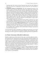
rated from its neighboring nodes by deleting all incoming edges. Figure 2.11 shows
that the node connectivity of a network can be smaller than its edge connectivity.
Fig. 2.11 Network with node
connectivity 1, edge
connectivity 2, and degree 4.
The smallest degree of a node
is 3
The flexibility of a network can be captured by the notion of embedding.Let
G = (V, E) and G

= (V

, E

) be two networks. An embedding of G

into G
assigns each node of G

to a node of G such that different nodes of G

are mapped

to different nodes of G and such that edges between two nodes in G

are also present
between their associated nodes in G [19]. An embedding of G

into G can formally
be described by a mapping function σ : V

→ V such that the following holds:
• if u = v for u,v ∈ V

, then σ (u) = σ (v) and
• if (u,v) ∈ E

, then (σ (u),σ(v)) ∈ E.
If a network G

can be embedded into a network G, this means that G is at least as
flexible as G

, since any algorithm that is based on the network structure of G

, e.g.,
by using edges between nodes for communication, can be re-formulated for G with
the mapping function σ , thus using corresponding edges in G for communication.
The network of a parallel system should be designed to meet the requirements
formulated for the architecture of the parallel system based on typical usage pat-
terns. Generally, the following topological properties are desirable:
• a small diameter to ensure small distances for message transmission,
• a small node degree to reduce the hardware overhead for the nodes,

• a large bisection bandwidth to obtain large data throughputs,
32 2 Parallel Computer Architecture
• a large connectivity to ensure reliability of the network,
• embedding into a large number of networks to ensure flexibility, and
• easy extendability to a larger number of nodes.
Some of these properties are conflicting and there is no network that meets all
demands in an optimal way. In the following, some popular direct networks are
presented and analyzed. The topologies are illustrated in Fig. 2.12. The topological
properties are summarized in Table 2.2.
2.5.2 Direct Interconnection Networks
Direct interconnection networks usually have a regular structure which is transferred
to their graph representation G = (V, E). In the following, we use n =|V | for the
number of nodes in the network and use this as a parameter of the network type
considered. Thus, each network type captures an entire class of networks instead of
a fixed network with a given number of nodes.
A complete graph is a network G in which each node is directly connected with
every other node, see Fig. 2.12(a). This results in diameter δ(G) = 1 and degree
g(G) = n − 1. The node and edge connectivity is nc(G) = ec(G) = n −1, since a
node can only be disconnected by deleting all n − 1 adjacent edges or neighboring
nodes. For even values of n, the bisection bandwidth is B(G) = n
2
/4: If two subsets
of nodes of size n/2 each are built, there are n/2 edges from each of the nodes of
one subset into the other subset, resulting in n/2·n/2 edges between the subsets. All
other networks can be embedded into a complete graph, since there is a connection
between any two nodes. Because of the large node degree, complete graph networks
can only be built physically for a small number of nodes.
In a linear array network, nodes are arranged in a sequence and there is a
bidirectional connection between any pair of neighboring nodes, see Fig. 2.12(b),
i.e., it is V ={v

1
, ,v
n
} and E ={(v
i
,v
i+1
) | 1 ≤ i < n}. Since n − 1 edges
have to be traversed to reach v
n
starting from v
1
, the diameter is δ(G) = n − 1.
The connectivity is nc(G) = ec(G) = 1, since the elimination of one node or edge
disconnects the network. The network degree is g(G) = 2 because of the inner
nodes, and the bisection bandwidth is B(G) = 1. A linear array network can be
embedded in nearly all standard networks except a tree network, see below. Since
there is a link only between neighboring nodes, a linear array network does not
provide fault tolerance for message transmission.
In a ring network, nodes are arranged in ring order. Compared to the linear array
network, there is one additional bidirectional edge from the first node to the last
node, see Fig. 2.12(c). The resulting diameter is δ(G) =

n/2

, the degree is g(G) =
2, the connectivity is nc(G) = ec(G) = 2, and the bisection bandwidth is also
B(G) = 2. In practice, ring networks can be used for small number of processors
and as part of more complex networks.
A d-dimensional mesh (also called d-dimensional array)ford ≥ 1 consists

of n = n
1
· n
2
· · n
d
nodes that are arranged as a d-dimensional mesh, see
2.5 Interconnection Networks 33
i)
(110,1)
(110,0)
(010,1)
(010,2)
(111,1)
(110,2)
(111,2)
(011,2)
(011,1)
(100,2)
(100,0)
(000,1)
(000,2)
(001,2)
(001,1)
(101,2)
(100,1)
(101,0)
(101,1)
(001,0)(000,0)
(010,0)

(011,0)
(111,0)
000 001
010 011
100 101
110 111
1111
1101
1011
0100
1000
1010
1110
1001
00010000
0010 0011
0110 0111
0101
1100
h)
1
23
4567
001
011
101100
111110
010
000
10

00
11
01
1
f)
0
1
2
3
4
5
a)
(1,1) (1,2) (1,3)
(2,3)(2,2)(2,1)
(3,2) (3,3)(3,1)
(1,2) (1,3)
(2,3)(2,2)(2,1)
(3,2) (3,3)(3,1)
(1,1)
12345
1
2
3
4
5
g)
b)
e)
d)
c)

Fig. 2.12 Static interconnection networks: (a) complete graph, (b) linear array, (c) ring, (d)two-
dimensional mesh, (e) two-dimensional torus, (f) k-dimensional cube for k=1,2,3,4, (g) cube-
connected-cycles network for k = 3, (h) complete binary tree, (i) shuffle–exchange network with
8 nodes, where dashed edges represent exchange edges and straight edges represent shuffle edges
34 2 Parallel Computer Architecture
Table 2.2 Summary of important characteristics of static interconnection networks for selected
topologies
Degree Diameter Edge- connectivity Bisection bandwidth
Network G with n nodes g(G) δ(G) ec(G) B(G)
Complete graph n − 11 n − 1

n
2

2
Linear array 2 n − 11 1
Ring 2

n
2

22
d-Dimensional mesh 2dd(
d
√
n − 1) dn
d−1
d
(n = r
d

)
d-Dimensional torus 2dd

d
√
n
2

2d 2n
d−1
d
(n = r
d
)
k-Dimensional hyper- logn log n log n
n
2
cube (n = 2
k
)
k-Dimensional 3 2k − 1 +

k/2

3
n
2k
CCC network
(n = k2
k

for k ≥ 3)
Complete binary 3 2 log
n+1
2
11
tree (n = 2
k
−1)
k-ary d-cube 2dd

k
2

2d 2k
d−1
(n = k
d
)
Fig. 2.12(d). The parameter n
j
denotes the extension of the mesh in dimension j
for j = 1, ,d. Each node in the mesh is represented by its position (x
1
, ,x
d
)
in the mesh with 1 ≤ x
j
≤ n
j

for j = 1, ,d. There is an edge between node
(x
1
, ,x
d
) and (x

1
, x

d
), if there exists μ ∈{1, ,d} with
|x
μ
− x

μ
|=1 and x
j
= x

j
for all j = μ.
In the case that the mesh has the same extension in all dimensions (also called
symmetric mesh), i.e., n
j
= r =
d
√
n for all j = 1, ,d, and therefore n =

r
d
, the network diameter is δ(G) = d · (
d
√
n − 1), resulting from the path length
between nodes on opposite sides of the mesh. The node and edge connectivity is
nc(G) = ec(G) = d, since the corner nodes of the mesh can be disconnected by
deleting all d incoming edges or neighboring nodes. The network degree is g(G) =
2d, resulting from inner mesh nodes which have two neighbors in each dimension.
A two-dimensional mesh has been used for the Teraflop processor from Intel, see
Sect. 2.4.3.
A d-dimensional torus is a variation of a d-dimensional mesh. The difference is
the additional edges between the first and the last node in each dimension, i.e., for
each dimension j = 1, ,d there is an edge between node (x
1
, ,x
j−1
, 1, x
j+1
,
, x
d
) and (x
1
, ,x
j−1
, n
j
, x

j+1
, ,x
d
), see Fig. 2.12(e). For the symmetric
case n
j
=
d
√
n for all j = 1, ,d, the diameter of the torus network is δ(G) =
d ·
d
√
n/2. The node degree is 2d for each node, i.e., g(G) = 2d. Therefore, node
and edge connectivities are also nc(G) = ec(G) = 2d.
A k-dimensional cube or hypercube consists of n = 2
k
nodes which are
connected by edges according to a recursive construction, see Fig. 2.12(f). Each
2.5 Interconnection Networks 35
node is represented by a binary word of length k, corresponding to the numbers
0, ,2
k
−1. A one-dimensional cube consists of two nodes with bit representations
0 and 1 which are connected by an edge. A k-dimensional cube is constructed
from two given (k − 1)-dimensional cubes, each using binary node representa-
tions 0, ,2
k−1
−1. A k-dimensional cube results by adding edges between each
pair of nodes with the same binary representation in the two (k − 1)-dimensional

cubes. The binary representations of the nodes in the resulting k-dimensional
cube are obtained by adding a leading 0 to the previous representation of the
first (k − 1)-dimensional cube and adding a leading 1 to the previous represen-
tations of the second (k − 1)-dimensional cube. Using the binary representations
of the nodes V ={0, 1}
k
, the recursive construction just mentioned implies that
there is an edge between node α
0
α
j
α
k−1
and node α
0
¯α
j
α
k−1
for
0 ≤ j ≤ k − 1 where ¯α
j
= 1forα
j
= 0 and ¯α
j
= 0forα
j
= 1. Thus,
there is an edge between every pair of nodes whose binary representation dif-

fers in exactly one bit position. This fact can also be captured by the Hamming
distance.
The Hamming distance of two binary words of the same length is defined as
the number of bit positions in which their binary representations differ. Thus, two
nodes of a k-dimensional cube are directly connected, if their Hamming distance is
1. Between two nodes v, w ∈ V with Hamming distance d,1≤ d ≤ k, there exists
a path of length d connecting v and w. This path can be determined by traversing
the bit representation of v bitwise from left to right and inverting the bits in which
v and w differ. Each bit inversion corresponds to a traversal of the corresponding
edge to a neighboring node. Since the bit representation of any two nodes can differ
in at most k positions, there is a path of length ≤ k between any pair of nodes. Thus,
the diameter of a k-dimensional cube is δ(G) = k. The node degree is g(G) = k,
since a binary representation of length k allows k bit inversions, i.e., each node has
exactly k neighbors. The node and edge connectivity is nc(G) = ec(G) = k as will
be described in the following.
The connectivity of a hypercube is at most k, i.e., nc(G) ≤ k, since each node
can be completely disconnected from its neighbors by deleting all k neighbors or
all k adjacent edges. To show that the connectivity is at least k, we show that there
are exactly k independent
paths between any pair of nodes v and w. Two paths are
independent of each other if they do not share any edge, i.e., independent paths
between v and w only share the two nodes v and w. The independent paths are
constructed based on the binary representations of v and w, which are denoted
by A and B, respectively, in the following. We assume that A and B differ in l
positions, 1 ≤ l ≤ k, and that these are the first l positions (which can be obtained
by a renumbering). We can construct l paths of length l each between v and w by
inverting the first l bits of A in different orders. For path i,0≤ i < l, we stepwise
invert bits i, ,l −1 in this order first, and then invert bits 0, ,i −1 in this order.
This results in l independent paths. Additional k −l independent paths between v
and w of length l +2 each can be constructed as follows: For i with 0 ≤ i < k −l,

we first invert the bit (l +i)ofA and then the bits at positions 0, ,l −1
stepwise.
Finally, we invert the bit (l +i) again, obtaining bit representation B. This is shown
36 2 Parallel Computer Architecture
010
110
000
001
101
111
011
100
Fig. 2.13 In a three-dimensional cube network, we can construct three independent paths (from
node 000 to node 110). The Hamming distance between node 000 and node 110 is l = 2. There are
two independent paths between 000 and 110 of length l = 2: path (000, 100, 110) and path (000,
010, 110). Additionally, there are k −l = 1 path of length l +2 = 4: path (000, 001, 101, 111, 110)
in Fig. 2.13 for an example. All k paths constructed are independent of each other,
showing that nc(G) ≥ k holds.
A k-dimensional cube allows the embedding of many other networks as will be
shown in the next subsection.
A cube-connected cycles (CCC) network results from a k-dimensional cube by
replacing each node with a cycle of k nodes. Each of the nodes in the cycle has
one off-cycle connection to one neighbor of the original node of the k-dimensional
cube, thus covering all neighbors, see Fig. 2.12(g). The nodes of a CCC network
can be represented by V ={0, 1}
k
×{0, ,k − 1} where {0, 1}
k
are the binary
representations of the k-dimensional cube and i ∈{0, ,k − 1} represents the

position in the cycle. It can be distinguished between cycle edges F and cube
edges E:
F ={((α, i), (α, (i +1) mod k)) | α ∈{0, 1}
k
, 0 ≤ i < k},
E ={((α, i), (β,i)) | α
i
= β
i
and α
j
= β
j
for j = i}.
Each of the k·2
k
nodes of the CCC network has degree g(G) = 3, thus eliminating a
drawback of the k-dimensional cube. The connectivity is nc(G) = ec(G) = 3 since
each node can be disconnected by deleting its three neighboring nodes or edges. An
upper bound for the diameter is δ(G) = 2k −1 +k/2. To construct a path of this
length, we consider two nodes in two different cycles with maximum hypercube
distance k. These are nodes (α, i) and (β, j)forwhichα and β differ in all k bits.
We construct a path from (α, i)to(β, j) by sequentially traversing a cube edge
and a cycle edge for each bit position. The path starts with (α
0
α
i
α
k−1
, i) and

reaches the next node by inverting α
i
to ¯α
i
= β
i
.From(α
0
β
i
α
k−1
, i) the next
node (α
0
β
i
α
k−1
, (i +1) mod k) is reached by using a cycle edge. In the next
steps, the bits α
i+1
, ,α
k−1
and α
0
, ,α
i−1
are successively inverted in this way,
using a cycle edge between the steps. This results in 2k − 1 edge traversals. Using

at most k/2additional traversals of cycle edges starting from (β,i +k −1modk)
leads to the target node (β, j).
A complete binary tree network has n = 2
k
− 1 nodes which are arranged as
a binary tree in which all leaf nodes have the same depth, see Fig. 2.12(h). The
2.5 Interconnection Networks 37
degree of inner nodes is 3, leading to a total degree of g(G) = 3. The diameter of
the network is δ(G) = 2 · log
n+1
2
and is determined by the path length between
two leaf nodes in different subtrees of the root node; the path consists of a subpath
from the first leaf to the root followed by a subpath from the root to the second leaf.
The connectivity of the network is nc(G) = ec(G) = 1, since the network can be
disconnected by deleting the root or one of the edges to the root.
A k-dimensional shuffle–exchange network has n = 2
k
nodes and 3·2
k−1
edges
[167]. The nodes can be represented by k-bit words. A node with bit representation
α is connected with a node with bit representation β,if
• α and β differ in the last bit (exchange edge)or
• α results from β by a cyclic left shift or a cyclic right shift (shuffle edge).
Figure 2.12(i) shows a shuffle–exchange network with 8 nodes. The permutation
(α, β) where β results from α by a cyclic left shift is called perfect shuffle.
The permutation (α, β) where β results from α by a cyclic right shift is called
inverse perfect shuffle, see [115] for a detailed treatment of shuffle–exchange
networks.

A k-ary d-cube with k ≥ 2 is a generalization of the d-dimensional cube with
n = k
d
nodes where each dimension i with i = 0, ,d −1 contains k nodes. Each
node can be represented by a word with d numbers (a
0
, ,a
d−1
) with 0 ≤ a
i
≤
k −1, where a
i
represents the position of the node in dimension i, i = 0, ,d −1.
Two nodes A = (a
0
, ,a
d−1
) and B = (b
0
, ,b
d−1
) are connected by an edge if
there is a dimension j ∈{0, ,d −1} for which a
j
= (b
j
±1) mod k and a
i
= b

i
for all other dimensions i = 0, ,d − 1, i = j.Fork = 2, each node has one
neighbor in each dimension, resulting in degree g(G) = d.Fork > 2, each node
has two neighbors in each dimension, resulting in degree g(G) = 2d.Thek-ary
d-cube captures some of the previously considered topologies as special case: A
k-ary 1-cube is a ring with k nodes, a k-ary 2-cube is a torus with k
2
nodes, a 3-ary
3-cube is a three-dimensional torus with 3 × 3 × 3 nodes, and a 2-ary d-cube is a
d-dimensional cube.
Table 2.2 summarizes important characteristics of the network topologies
described.
2.5.3 Embeddings
In this section, we consider the embedding of several networks into a hypercube
network, demonstrating that the hypercube topology is versatile and flexible.
2.5.3.1 Embedding a Ring into a Hypercube Network
For an embedding of a ring network with n = 2
k
nodes represented by V

=
{1, ,n} in a k-dimensional cube with nodes V ={0, 1}
k
, a bijective function
from V

to V is constructed such that a ring edge (i, j) ∈ E

is mapped to a hyper-
cube edge. In the ring, there are edges between neighboring nodes in the sequence

38 2 Parallel Computer Architecture
1, ,n. To construct the embedding, we have to arrange the hypercube nodes
in V in a sequence such that there is also an edge between neighboring nodes in
the sequence. The sequence is constructed as reflected Gray code (RGC) sequence
which is defined as follows:
A k-bit RGC is a sequence with 2
k
binary strings of length k such that two neigh-
boring strings differ in exactly one bit position. The RGC sequence is constructed
recursively, as follows:
• The 1-bit RGC sequence is RGC
1
= (0, 1).
• The 2-bit RGC sequence is obtained from RGC
1
by inserting a 0 and a 1 in front
of RGC
1
, resulting in the two sequences (00, 01) and (10, 11). Reversing the
second sequence and concatenation yields RGC
2
= (00, 01, 11, 10).
• For k ≥ 2, the k-bit Gray code RGC
k
is constructed from the (k − 1)-bit Gray
code RGC
k−1
= (b
1
, ,b

m
) with m = 2
k−1
where each entry b
i
for 1 ≤ i ≤ m
is a binary string of length k −1. To construct RGC
k
,RGC
k−1
is duplicated; a 0
is inserted in front of each b
i
of the original sequence, and a 1 is inserted in front
of each b
i
of the duplicated sequence. This results in sequences (0b
1
, ,0b
m
)
and (1b
1
, ,1b
m
). RGC
k
results by reversing the second sequence and concate-
nating the two sequences; thus RGC
k

= (0b
1
, ,0b
m
, 1b
m
, ,1b
1
).
The Gray code sequences RGC
k
constructed in this way have the property that
they contain all binary representations of a k-dimensional hypercube, since the
construction corresponds to the construction of a k-dimensional cube from two
(k − 1)-dimensional cubes as described in the previous section. Two neighboring
k-bit words of RGC
k
differ in exactly one bit position, as can be shown by induc-
tion. The statement is surely true for RGC
1
. Assuming that the statement is true for
RGC
k−1
,itistrueforthefirst2
k−1
elements of RGC
k
as well as for the last 2
k−1
elements, since these differ only by a leading 0 or 1 from RGC

k−1
. The statement
is also true for the two middle elements 0b
m
and 1b
m
at which the two sequences
of length 2
k−1
are concatenated. Similarly, the first element 0b
1
and the last element
1b
1
of RGC
k
differ only in the first bit. Thus, neighboring elements of RGC
k
are
connected by a hypercube edge.
An embedding of a ring into a k-dimensional cube can be defined by the mapping
σ : {1, ,n}→{0, 1}
k
with σ (i):= RGC
k
(i),
where RGC
k
(i) denotes the ith element of RGC
k

. Figure 2.14(a) shows an example
for k = 3.
2.5.3.2 Embedding a Two-Dimensional Mesh into a Hypercube Network
The embedding of a two-dimensional mesh with n = n
1
· n
2
nodes into a k-
dimensional cube with n = 2
k
nodes can be obtained by a generalization of the
embedding of a ring network. For k
1
and k
2
with n
1
= 2
k
1
and n
2
= 2
k
2
, i.e.,
k
1
+k
2

= k, the Gray codes RGC
k
1
= (a
1
, ,a
n
1
) and RGC
k
2
= (b
1
, ,b
n
2
)are
2.5 Interconnection Networks 39
Fig. 2.14 Embeddings into a
hypercube network: (a)
embedding of a ring network
with 8 nodes into a
three-dimensional hypercube
and (b) embedding of a
two-dimensional 2 × 4mesh
into a three-dimensional
hypercube
010
000
001

101
111
011
100
110
110 111 101 10
0
010 011 001 00
0
001 011 010
010
110
000
001
101
111
011
100
111101100
11
0
000
a)
b)
used to construct an n
1
×n
2
matrix M whose entries are k-bit strings. In particular,
it is

M =
⎡
⎢
⎢
⎢
⎣
a
1
b
1
a
1
b
2
a
1
b
n
2
a
2
b
1
a
2
b
2
a
2
b

n
2
.
.
.
.
.
.
.
.
.
.
.
.
a
n
1
b
1
a
n
1
b
2
a
n
1
b
n
2

⎤
⎥
⎥
⎥
⎦
.
The matrix is constructed such that neighboring entries differ in exactly one bit
position. This is true for neighboring elements in a row, since identical elements
of RGC
k
1
and neighboring elements of RGC
k
2
are used. Similarly, this is true for
neighboring elements in a column, since identical elements of RGC
k
2
and neighbor-
ing elements of RGC
k
1
are used. All elements of M are bit strings of length k and
there are no identical bit strings according to the construction. Thus, the matrix M
contains all bit representations of nodes in a k-dimensional cube and neighboring
entries in M correspond to neighboring nodes in the k-dimensional cube, which are
connected by an edge. Thus, the mapping
σ : {1, ,n
1
}×{1, ,n

2
}→{0, 1}
k
with σ (i, j) = M(i, j)
is an embedding of the two-dimensional mesh into the k-dimensional cube.
Figure 2.14(b) shows an example.
2.5.3.3 Embedding of a d-Dimensional Mesh into a Hypercube Network
In a d-dimensional mesh with n
i
= 2
k
i
nodes in dimension i,1≤ i ≤ d, there are
n = n
1
·····n
d
nodes in total. Each node can be represented by its mesh coordinates
(x
1
, ,x
d
) with 1 ≤ x
i
≤ n
i
. The mapping