The boundary element method with programming for engineers and scientists - phần 7 ppsx
Bạn đang xem bản rút gọn của tài liệu. Xem và tải ngay bản đầy đủ của tài liệu tại đây (396.83 KB, 50 trang )
294 The Boundary Element Method with Programming
region interfaces. There are two approaches which can be taken in the implementation of
the method.
In the first, we modify the assembly procedure, so that a larger system of equations is
now obtained including the additional unknowns at the interfaces. The second method is
similar to the approach taken by the finite element method. Here we construct a
“stiffness matrix”, K, of each region, the coefficients of which are the fluxes or tractions
due to unit temperatures/displacements. The matrices K for all regions are then
assembled in the same way as with the FEM. The second method is more efficient and
more amenable to implementation on parallel computers. The method may also be used
for coupling boundary with finite elements, as outlined in Chapter 12. We will therefore
only discuss the second method here. For the explanation of the first approach the reader
is referred for appropriate text books
2,3
.
11.2 STIFFNESS MATRIX ASSEMBLY
The multi-region assembly is not very efficient in cases where sequential
excavation/construction (for example, in tunnelling) is to be modelled, since the
coefficient matrices of all regions have to be computed and assembled every time a
region is added or removed. Also, the method is not suitable for parallel processing since
there the region matrices must be assembled and computed completely separately.
Finally, significant efficiency gains can be made with the proposed method where only
some nodes of the region are connected to other regions.
The stiffness matrix assembly, utilises a philosophy similar to that used by the finite
element method. The idea is to compute a “stiffness matrix” K
N
for each region N.
Coefficients of K
N
are values of t due to unit values of u at all region nodes. In potential
flow problems these would correspond to fluxes due to unit temperatures while in
elasticity they would be tractions due to unit displacements. To obtain the “stiffness
matrix” K
N
of a region, we simply solve the Dirichlet problem M times, where M is the
number of degrees of freedom of the BE region nodes. For example, to get the first
column of K
N
, we apply a unit value of temperature or of displacement in x-direction, as
shown in Figure 11.1 while setting all other node values to zero.
Figure 11.1
Example of computation of “stiffness coefficients”: Cantilever beam subjected to a
unit displacement
1
x
u showing the traction distribution obtained from Program 7.1
1
x
u
x
t
MULTIPLE REGIONS 295
For computation of Dirichlet problems we use equation (7.3), with a modified right
hand side
(11.1)
Here
>
@
>
@
,TU''are the assembled coefficient matrices,
^`
1
t is the first column of the
stiffness matrix K
M
and
^
`
1
u is a vector with a unit value in the first row ,i.e
(11.2)
If we perform the multiplication of
>
@
^`
1
Tu' it can be easily seen that the right hand
side of equation (11.1) is simply the first column of matrix
>
@
T' . The computation of
the region “stiffness matrix” is therefore basically a solution of
>
@
^` ^ `
ii
Ut F' , with
N right hand sides
^`
i
F
, where each right hand side corresponds to a column in
>
@
T' .
Each solution vector
^`
i
t represents a column in K , i.e.,
(11.3)
For each region (N) we have the following relationship between {t} and {u}:
(11.4)
To compute, for example, the problem of heat flow past an isolator, which is not
impermeable but has conductivity different to the infinite domain, we specify two
regions, an infinite and a finite one, as shown in figure 11.2. Note that the outward
normals of the two regions point in directions opposite to each other (Figure 11.3). First
we compute matrices K
I
and K
II
for each region separately and then we assemble the
regions using the conditions for flow balance and uniqueness of temperature in the case
of potential problems and equilibrium and compatibility in the case of elasticity. These
conditions are written as
(11.5)
The assembled system of equations for the example in Figure 11.2 is simply:
(11.6)
>
@
^
`
>
@
^
`
11
Ut Tu' '
^`
1
1
0
0
u
½
°°
°°
®¾
°°
°°
¯¿
#
^` ^`
12
N
tt
ªº
¬¼
K "
^` ^ `
NN
N
tu K
^` ^` ^` ^ ` ^ `
;
III I II
tt t u u
^`
^`
III
tu KK
296 The Boundary Element Method with Programming
which can be solved for
^`
u if
^`
t is known.
Figure 11.2
Example of a multi-region analysis: inclusion with different conductivity in an
infinite domain
Figure 11.3 The two regions of the problem
11.2.1 Partially coupled problems
In many cases we have problems where not all nodes of the regions are connected (these
are known as partially coupled problems). Consider for example the modified heat flow
1
Re
g
ion II,
k
2
2
3
4
5
6
7
8
Region I, k
1
1
2
3
4
5
6
7
8
1
2
3
4
5
6
7
8
n
n
Region I (infinite)
Region II (finite)
MULTIPLE REGIONS 297
problem in Figure 11.4 where an additional circular impermeable isolator is specified on
the right hand side.
Figure 11.4
Problem with a circular inclusion and an isolator
Here only some of the nodes of region I are connected to region II. It is obviously
more efficient to consider in the calculation of the stiffness matrix only the interface
nodes, i.e. only of those nodes that are connected to a region. It is therefore proposed
that we modify our procedure in such a way that we first solve the problem with zero
values of u at the interface between region I and II and then solve the problem where
unit values of u are applied at each node in turn.
For partially coupled problems we therefore have to solve the following types of
problems (this is explained on a heat flow problem but can be extended to elasticity
problems by replacing t with t and u with u):
1. Solution of system with “fixed” interface nodes
The first one is where boundary conditions are applied at the nodes which are not
connected to other regions (free nodes) and Dirichlet boundary conditions with
zero prescribed values are applied at the nodes which are connected to other
regions (coupled nodes). For each region we can write the following system of
equations:
(11.7)
>@
^`
^`
^`
0
0
0
N
N
N
c
N
f
t
BF
x
½
°°
®¾
°°
¯¿
1
Region II, k
2
2
3
4
5
6
7
8
Region I, k
1
9
10
11
12
13
14
15
16
298 The Boundary Element Method with Programming
where
>@
N
B is the assembled left hand side and
^`
N
o
F
contains the right hand side
due to given boundary conditions for region N. Vector
^`
N
co
t contains the heat flow
at the coupled nodes and vector
^`
N
f
o
x
either temperatures or heat flow at the free
nodes of region
N, depending on the boundary conditions prescribed (Dirichlet or
Neumann).
2. Solution of system with unit values applied at the interface nodes
The second problem to be solved for each region is to obtain the solution due to
Dirichlet boundary condition of unit value applied at each of the interface nodes in
turn and zero prescribed values at the free nodes. The equations to be solved are
(11.8)
where
^`
N
n
F
is the right hand side computed for a unit value of u at node n. The
vector
^`
N
cn
t contains the heat flow at the coupled nodes and
^`
N
f
n
x
the temperature
or heat flow at the free nodes, for the case of unit
Dirichlet boundary conditions at
node n. N
c
equations are obtained where N
c
is the number of interface nodes in the
case of the potential problem (in the case of elasticity problems it refers to the
number of interface degrees of freedom). Note that the left hand side of the system
of equations, [
B]
N
, is the same for the first and second problem and that
^`
n
F
simply corresponds to the n
th
column of
>
@
T' .
After the solution of the first two problems
^`
N
c
t and
^`
N
f
x
can be expressed in terms of
^`
N
c
u by:
(11.9)
where
^`
N
c
u contains the temperatures at the interface nodes of region N and the
matrices
N
K
and
N
A
are defined by:
(11.10)
^`
^`
^`
^`
^`
0
0
NN
N
N
cc
c
NN
N
ff
tt
u
xx
½ ½
ªº
°°° °
«»
®¾® ¾
«»
°°° °
¬¼
¯¿¯ ¿
K
A
>@
^`
^`
^`
1, 2
N
N
cn
c
n
N
fn
t
BFnN
x
½
°°
®¾
°°
¯¿
!
^` ^` ^ ` ^ `
11
;
cc
NN
NN
ccN c cN
tt xx
ªºª º
«»« »
¬¼¬ ¼
KA""
MULTIPLE REGIONS 299
3. Assembly of regions, calculation of interface unknowns
After all the region stiffness matrices K
N
have been computed they are assembled
to a system of equations which can be solved for the unknown
^`
c
u .
For the assembly we use conditions of heat balance and uniqueness of temperature
or equilibrium and compatibility as discussed previously. This results in the
following system of equations
(11.11)
where [K] is the assembled “stiffness matrix” of the interface nodes and {
F}is the
assembled right hand side. This system is solved for the unknown
^`
c
u at the nodes
of all interfaces of the problem.
4. Calculation of unknowns at the free nodes of region N
After the interface unknown have been determined the values of
t at the interface
(
^`
N
c
t ) and the value of u or t at the free nodes (
^`
N
f
x
) are determined for each
region by the application of
(11.12)
Note that
^`
N
c
u is obtained by gathering values from the vector of unknown at all
the interfaces
^`
c
u .
11.2.2 Example
The procedure is explained in more detail on a simple example in potential flow.
Consider the example in Figure 11.5 which contains two homogeneous regions.
Dirichlet boundary conditions with prescribed zero values are applied on the left side
and Neuman BC’s on the right side as shown. All other boundaries are assumed to have
Neuman BC with zero prescribed values. The interface only involves nodes 2 and 3 and
therefore only 2 interface unknowns exist.
For an efficient implementation it will be necessary to renumber the nodes for each
region, i.e. introduce a separate local numbering for each region. This will not only
allow each region to be treated completely independently but also save storage space,
because nodes not on the interface will belong to one region only.
>@
^` ^ `
c
uF K
^`
^`
^`
^`
^`
0
0
NN
N
N
cc
c
NN
N
ff
tt
u
xx
½ ½
ªº
°°° °
«»
®¾® ¾
«»
°°° °
¬¼
¯¿¯ ¿
K
A
300 The Boundary Element Method with Programming
Figure 11.5
Example for stiffness assembly, partially coupled problem with global node
numbering; local (element) numbering shown in italics.
Figure 11.6 The different problems to be solved for regions I and II (potential problem)
On the top of Figure 11.6 we show the local (region) numbering that is adapted for
region I and II. The sequence in which the nodes of the region are numbered is such that
the interface nodes are numbered first. We also depict in the same figure the problems
u= 0
u= 0
u= 0
Region I
u= 0
t= t
0
Region II
4
1
2
3
2
1
3
4
I
t
10
I
t
20
II
t
20
II
t
10
I
t
11
I
t
12
I
t
21
I
t
22
II
t
22
II
t
21
II
t
12
II
t
11
1
1
I
u
2
1
II
u
2
0
I
u
1
1
II
u
1
0
I
u
2
1
I
u
1
0
I
u
2
1
I
u
1
4
2
Re
g
ion I
1
3
4
5
6
7
8
5
6
Region II
2
3
0 u
0
tt
1
2
1
2
1
2
1
2
1
2
1
2
1
2
1
2
MULTIPLE REGIONS 301
which have to be solved for obtaining vector
^`
co
t and the two rows of matrix K and A.
It is obvious that for the first problem to be solved for region
I , where for all nodes u=0,
^`
co
t will also be zero. Following the procedure in chapter 7 and referring to the
element numbering of Figure 11.5 we obtain the following integral equations for the
second and third problem for region
I.
(11.13)
for
i=1,2,3,4. In Equation 11.13, two subscripts have been introduced for t: the first
subscript refers to the node number where t is computed and the second to the node
number where the unit value of
u is applied. The roman superscript refers to the region
number. The notation for
and UT''is the same as defined in Chapter 7, i.e. the first
subscript defines the node number and the second the collocation point number; the
superscript refers to the boundary element number (in square areas in Figure 11.5).
This gives the following system of equations with two right hand sides
(11.14)
After solving the system of equations we obtain
(11.15)
where
(11.16)
22 44 12
2 111 221 131 241 2 1
22 2 4 4 3 2
3 112 222 132 242 1 2
1 1
1 1
IIII
iiii ii
II I
iiii ii
uUtUtUtUtTT
uUtUtUtUtTT
' ' ' ' ''
' ' ' ' ''
^` ^` ^` ^`
I
I
II
I
I
cfcc
; uAxuKt
^` ^ `
^`
II
11 12 1
1
2
21 22 2
I
33132
44142
;;
;
II I
I
I
cc
II I
III
I
f
III
tt u
t
tu
t
tt u
ttt
x
ttt
ªº ½
½
°° ° °
«»
®¾ ® ¾
«»
°°
°°
¯¿
¬¼ ¯¿
½ ª º
°°
«»
®¾
«»
°°
¯¿ ¬ ¼
K
A
°
°
°
¿
°
°
°
¾
½
°
°
°
¯
°
°
°
®
''''
''''
''''
''''
°
°
°
¿
°
°
°
¾
½
°
°
°
¯
°
°
°
®
»
»
»
»
»
»
¼
º
«
«
«
«
«
«
¬
ª
''' '
''''
''' '
''' '
2
14
1
24
2
14
1
24
2
13
1
23
2
13
1
23
2
12
1
22
2
12
1
22
3
11
2
21
2
11
1
21
4241
3231
2221
1211
4
24
4
14
1
24
2
14
4
23
4
13
2
23
2
13
4
22
4
12
2
22
2
12
4
21
4
11
2
21
2
11
T
T
T
T
T
T
T
T
T
T
T
T
T
T
T
T
t
t
t
t
t
t
t
t
U
U
U
U
U
U
U
U
U
U
U
U
U
U
U
U
I
I
I
I
I
I
I
I
302 The Boundary Element Method with Programming
where
^`
c
t and
^`
c
u refer to the values of t and u at the interface.
For region II we have for the case of zero
u at the interface nodes
(11.17)
This gives
(11.18)
which can be solved for the values at the interface and free nodes
(11.19)
In our notation
^`
I
co
t refers to the values of t at the interface for the case where u=0 at
the interface.
^`
I
co
x
refers to the values of u at the free nodes (where Neumann boundary
conditions have been applied).
For
23
1 and 1uu we obtain
(11.20)
The solutions can be written as
(11.21)
°
°
°
¿
°
°
°
¾
½
°
°
°
¯
°
°
°
®
''
''
''
''
°
°
°
¿
°
°
°
¾
½
°
°
°
¯
°
°
°
®
»
»
»
»
»
»
¼
º
«
«
«
«
«
«
¬
ª
''''''
''''''
''''''
'''''
'
0
6
24
6
14
0
6
23
6
13
0
6
22
6
12
0
6
21
6
11
40
30
20
10
7
24
6
14
5
24
6
14
8
24
8
14
7
23
6
13
5
23
6
13
8
23
8
13
7
22
6
12
5
22
6
12
8
22
8
12
7
21
6
11
5
21
6
11
8
21
8
11
tUU
tUU
tUU
tUU
u
u
t
t
TTTTUU
TTTTUU
TTTTUU
TTTTUU
II
II
II
II
8865
220 110 1 2 30
67 6 6
1240 1 20
II II II
iiii
II
ii i i
Ut Ut T T u
TTu UUt
''''
' ' ' '
^` ^ `
II
10 20
0
40 30
;
II II
co f
II II
tu
tx
tu
½ ½
°° ° °
®¾ ® ¾
°° ° °
¯¿ ¯ ¿
88 65 67 58
1122221232124212
88 65 67 78
21122112311241 21
1
1
II II II II
iiii ii ii
II II II II
i i ii ii ii
Ut U t T T u T T u T T
Ut Ut T T u T T u T T
' ' '' '' ''
' ' '' '' ''
^` ^` ^` ^` ^` ^`
II II II II II II
II II
00
;
cc c f f c
tt u xx u KA
MULTIPLE REGIONS 303
where
(11.22)
The equations of compatibility or preservation of heat at the interface can be written
as
(11.23)
Substituting (11.16) and (11.22) into (11.23) we obtain
(11.24)
where
(11.25)
This system can be solved for the interface unknowns. The calculation of the other
unknowns is done separately for each region. For region I we have
(11.26)
Whereas for region II
(11.27)
If we consider the equivalent elasticity problem of a cantilever beam, we see (Figure
11.7) then for region
II the problem where the interface displacements are fixed gives
the tractions at the interface corresponding to a shortened cantilever beam. If
u
x
=1 is
applied only a rigid body motion results and therefore no resulting tractions at the
interface occur. The application of
u
y
=1 however will result in shear tractions at the
interface.
^` ^`
0
c
ut K
°
¿
°
¾
½
°
¯
°
®
°
¿
°
¾
½
°
¯
°
®
°
¿
°
¾
½
°
¯
°
®
°
¿
°
¾
½
°
¯
°
®
°
¿
°
¾
½
°
¯
°
®
3
2
1
2
2
1
1
2
2
1
0
u
u
u
u
u
u
;
t
t
t
t
II
c
II
c
I
c
I
c
II
c
II
c
I
c
I
c
^` ^` ^ `
^` ^`
II II I
1011112 1
20
22122 2
II II
30
33132
40
44142
;;;
;;
II
II II II II
II
ccoc
IIII II II II
IIII II II
II
cco
II
II II II
t
ttt u
ttu
tttt u
uuuu
xx
u
uuu
½
½ ª º ½
°° °° ° °
«»
®¾ ®¾ ® ¾
«»
°° ° °
°°
¯¿ ¬ ¼ ¯ ¿
¯¿
½
½ ª º
°° °°
«»
®¾ ®¾
«»
°°
°°
¯¿ ¬ ¼
¯¿
K
A
^` ^`
210
11 22 12 21
320
22 11 21 12
;;
I
IIIIII
c
IIIIIII
ut
tt tt
ut
uttttt
½ ½
ªº
°° °°
«»
®¾ ®¾
«»
°° °°
¬¼
¯¿ ¯¿
K
^` ^` ^` ^`
IIII
II
;
ccf c
tuxu KA
^` ^` ^` ^` ^` ^`
II II II II II II
II II
00
;
cc c f f c
tt u xx u KA
304 The Boundary Element Method with Programming
Figure 11.7
Effect of application of Dirichlet boundary conditions on region II of cantilever
beam (elasticity problem)
11.3 COMPUTER IMPLEMENTATION
We now consider the computer implementation of the stiffness matrix assembly method.
We divide this into two tasks. First we develop a SUBROUTINE Stiffness_BEM for the
calculation of matrix K. If the problem is not fully coupled, then this subroutine will
also determine the matrix
A
and the solutions for zero values of u at the interface.
Secondly we develop a program General_purpose_BEM_Multi.
For an efficient implementation (where zero entries in the matrices are avoided) we
must consider 3 different numbering systems, each one is related to the global
numbering system as shown in Figure 11.5:
1. Element numbering. This is the sequence in which the nodes to which an element
connects are entered in the element incidence vector. In the example in Figure 11.5
we have only two element nodes (
1,2). Table 11.1 has two main columns: One
termed “in global numbering” which shows the node numbers as they appear in
Figure 11.5 and the other termed “in region numbering” as they appear on the top of
Figure 11.6.
2. Region numbering. This numbering is used for computing the “stiffness matrix” of
a region. For this the element node numbers are specified in “region numbering”.
1
x
u
1
y
u
MULTIPLE REGIONS 305
Table 11.2 depicts the “region incidences” i.e. the sequence of node numbers of a
region.
3. Interface numbering. This is basically the sequence in which the interface nodes
are entered in the interface incidence vector. For the example problem the interface
incidences are given in Table 11.3. This sequence is determined in such a way that
the first node of the first interface element will start the sequence. Note that the
interface incidences are simply the first two values of the region incidence vector.
For problems involving more than one unknown per node the incidence vectors have to
be expanded to
Destination vectors as explained in Chapter 7.
Table 11.1
Incidences of boundary elements in global and local numbering
Table 11.2
Region incidences
1. 2. 3. 4.
Region I 2 3 4 1
Region II 3 2 5 6
Table 11.3 Interface incidences
1. 2.
Region I 2 3
Region II 3 2
.
in global numbering in region numbering
Boundary
Element
number
1. 2. 1. 2.
1 1 2 4 1
2 2 3 1 2
3 3 4 2 3
4 4 1 3 4
5 2 5 2 3
6 5 6 3 4
7 6 3 4 1
8 3 2 1 2
306 The Boundary Element Method with Programming
11.3.1 Subroutine Stiffness_BEM
The tasks for the Stiffness_BEM are essentially the same as for the
General_Purpose_BEM, except that the boundary conditions that are considered are
expanded. We add a new boundary code,2 , which is used to mark nodes at the interface.
The input parameters for SUBROUTINE Stiffness_BEM are the incidence vectors
of the boundary elements, which describe the boundary of the region, the coordinates of
the nodes and the Boundary conditions. Note that the vector of incidences as well as the
coordinates has to be in the local (region) numbering. SUBROUTINE AssemblySTIFF
is basically the same as SUBROUTINE Assembly, except that a boundary code 2 for
interface conditions has been added. Boundary code 2 is treated the same as code 1
(
Dirichlet) except that columns of ['T]
e
are assembled into the array RhsM (multiple
right hand sides). SUBROUTINE Solve is modified into Solve_Multi, which can
handle both single (Rhs) and multiple (RhsM) right hand sides.
The output parameter of the SUBROUTINE is stiffness matrix K and for partially
coupled problems in addition matrix A as well as {t}
c
. The rows and columns of these
matrices will be numbered in a local (interface) numbering. The values of
^`
0
f
u
and
^`
0c
t are stored in the array El_res which contains the element results. They can be
added at element level.
We show below the library module Stiffness_lib which contains all the necessary
declarations and subroutines for the computation of the stiffness matrix. The symmetry
option has been left out in the implementation shown to simplify the coding.
MODULE Stiffness_lib
USE Utility_lib ; USE Integration_lib ; USE Geometry_lib
IMPLICIT NONE
INTEGER :: Cdim ! Cartesian dimension
INTEGER :: Ndof ! No. of degeres of freedom per node
INTEGER :: Nodel ! No. of nodes per element
INTEGER :: Ndofe ! D.o.F´s / Elem
REAL :: C1,C2 ! material constants
INTEGER, ALLOCATABLE :: Bcode(:,:)
REAL, ALLOCATABLE :: Elres_u(:,:),Elres_t(:,:) ! El. results
CONTAINS
SUBROUTINE Stiffnes_BEM(Nreg,maxe,xP,incie,Ncode,Ndofc,KBE,A,TC)
!
! Computes the stiffness matrix of a boundary element region
! no symmetry implemented
!
INTEGER,INTENT(IN) :: Nreg ! Region code
INTEGER,INTENT(IN) :: maxe ! Number of boundary elements
REAL, INTENT(IN) :: xP(:,:) ! Array of node coordinates
INTEGER, INTENT(IN):: Incie(:,:) ! Array of incidences
INTEGER, INTENT(IN):: Ncode(:) ! Global restraint code
INTEGER, INTENT(IN):: Ndofc ! No of interface D.o.F.
MULTIPLE REGIONS 307
REAL(KIND=8), INTENT(OUT) :: KBE(:,:) ! Stiffness matrix
REAL(KIND=8), INTENT(OUT) :: A(:,:) ! u due to u
c
=1
REAL(KIND=8), INTENT(OUT) :: TC( :) ! t due to u
c
=0
INTEGER, ALLOCATABLE :: Ldeste(:,:)! Element destinations
REAL(KIND=8), ALLOCATABLE :: dUe(:,:),dTe(:,:),Diag(:,:)
REAL(KIND=8), ALLOCATABLE :: Lhs(:,:)
REAL(KIND=8), ALLOCATABLE :: Rhs(:),RhsM(:,:) ! right hand sides
REAL(KIND=8), ALLOCATABLE :: u1(:),u2(:,:) ! results
REAL, ALLOCATABLE :: Elcor(:,:)
REAL :: v3(3),v1(3),v2(3)
INTEGER :: Nodes,Dof,k,l,nel
INTEGER :: n,m,Ndofs,Pos,i,j,nd
Nodes= UBOUND(xP,2) ! total number of nodes of region
Ndofs= Nodes*Ndof ! Total degrees of freedom of region
ALLOCATE(Ldeste(maxe,Ndofe)) ! Elem. destination vector
!
! Determine Element destination vector
!
Elements:&
DO Nel=1,Maxe
k=0
DO n=1,Nodel
DO m=1,Ndof
k=k+1
IF(Ndof > 1) THEN
Ldeste(Nel,k)= ((Incie(Nel,n)-1)*Ndof + m)
ELSE
Ldeste(Nel,k)= Incie(Nel,n)
END IF
END DO
END DO
END DO &
Elements
ALLOCATE(dTe(Ndofs,Ndofe),dUe(Ndofs,Ndofe))
ALLOCATE(Diag(Ndofs,Ndof))
ALLOCATE(Lhs(Ndofs,Ndofs),Rhs(Ndofs),RhsM(Ndofs,Ndofs))
ALLOCATE(u1(Ndofs),u2(Ndofs,Ndofs))
ALLOCATE(Elcor(Cdim,Nodel))
!
! Compute and assemble element coefficient matrices
!
Lhs= 0
Rhs= 0
Elements_1:&
DO Nel=1,Maxe
Elcor(:,:)= xP(:,Incie(nel,:))! gather element coords
IF(Cdim == 2) THEN
IF(Ndof == 1) THEN
CALL Integ2P(Elcor,Incie(nel,:),Nodel,Nodes,xP,C1,dUe,dTe)
ELSE
CALL Integ2E(Elcor,Incie(nel,:),Nodel,Nodes&
308 The Boundary Element Method with Programming
,xP,C1,C2,dUe,dTe)
END IF
ELSE
CALL Integ3(Elcor,Incie(nel,:),Nodel,Nodes,xP,Ndof &
,C1,C2,dUe,dTe)
END IF
CALL AssemblyMR(Nel,Lhs,Rhs,RhsM,DTe,Due&
,Ldeste(nel,:),Ncode,Diag)
END DO &
Elements_1
!
! Add azimuthal integral for infinite regions
!
IF(Nreg == 2) THEN
DO m=1, Nodes
DO n=1, Ndof
k=Ndof*(m-1)+n
Diag(k,n) = Diag(k,n) + 1.0
END DO
END DO
END IF
!
! Add Diagonal coefficients
!
Nodes_global: &
DO m=1,Nodes
Degrees_of_Freedoms_node: &
DO n=1,Ndof
DoF = (m-1)*Ndof + n ! global degree of freedom no.
k = (m-1)*Ndof + 1 ! address in coeff. matrix (row)
l = k + Ndof - 1 ! address in coeff. matrix (column)
IF (NCode(DoF) == 1) THEN ! Dirichlet - Add Diagonal to Rhs
CALL Get_local_DoF(Maxe,Dof,Ldeste,Nel,Pos)
Rhs(k:l) = Rhs(k:l) - Diag(k:l,n)*Elres_u(Nel,Pos)
ELSE ! Neuman - Add Diagonal to Lhs
Lhs(k:l,Dof)= Lhs(k:l,Dof) + Diag(k:l,n)
END IF
END DO &
Degrees_of_Freedoms_node
END DO &
Nodes_global
! Solve problem
CALL Solve_Multi(Lhs,Rhs,RhsM,u1,u2)
!
! Gather element results due to
! “fixed” interface nodes
!
Elements2: &
DO nel=1,maxe
D_o_F1: &
DO nd=1,Ndofe
MULTIPLE REGIONS 309
IF(NCode(Ldeste(nel,nd)) == 0) THEN
Elres_u(nel,nd) = u1(Ldeste(nel,nd))
ELSE IF(NCode(Ldeste(nel,nd)) == 1) THEN
Elres_t(nel,nd) = u1(Ldeste(nel,nd))
END IF
END DO &
D_o_F1
END DO &
Elements2
!
! Gather stiffness matrix KBE and matrix A
!
Interface_DoFs: &
DO N=1,Ndofc
KBE(N,:)= u2(N,:)
TC(N)= u1(N)
END DO &
Interface_DoFs
Free_DoFs: &
DO N=Ndofc+1,Ndofs
A(N,:)= u2(N,:)
END DO &
Free_DoFs
DEALLOCATE (Ldeste,dUe,dTe,Diag,Lhs,Rhs,RhsM,u1,u2,Elcor)
RETURN
END SUBROUTINE Stiffnes_BEM
SUBROUTINE Solve_Multi(Lhs,Rhs,RhsM,u,uM)
!
! Solution of system of equations
! by Gauss Elimination
! for multple right hand sides
!
REAL(KIND=8) :: Lhs(:,:) ! Equation Left hand side
REAL(KIND=8) :: Rhs(:) ! Equation right hand side 1
REAL(KIND=8) :: RhsM(:,:) ! Equation right hand sides 2
REAL(KIND=8) :: u(:) ! Unknowns 1
REAL(KIND=8) :: uM(:,:) ! Unknowns 2
REAL(KIND=8) :: FAC
INTEGER M,Nrhs ! Size of system
INTEGER i,n,nr
M= UBOUND(RhsM,1) ; Nrhs= UBOUND(RhsM,2)
! Reduction
Equation_n: &
DO n=1,M-1
IF(ABS(Lhs(n,n)) < 1.0E-10) THEN
CALL Error_Message('Singular Matrix')
END IF
Equation_i: &
DO i=n+1,M
FAC= Lhs(i,n)/Lhs(n,n)
310 The Boundary Element Method with Programming
Lhs(i,n+1:M)= Lhs(i,n+1:M) - Lhs(n,n+1:M)*FAC
Rhs(i)= Rhs(i) - Rhs(n)*FAC
RhsM(i,:)= RhsM(i,:) - RhsM(n,:)*FAC
END DO &
Equation_i
END DO &
Equation_n
! Backsubstitution
Unknown_1: &
DO n= M,1,-1
u(n)= -1.0/Lhs(n,n)*(SUM(Lhs(n , n+1:M)*u(n+1:M)) - Rhs(n))
END DO &
Unknown_1
Load_case: &
DO Nr=1,Nrhs
Unknown_2: &
DO n= M,1,-1
uM(n,nr)= -1.0/Lhs(n,n)*(SUM(Lhs(n , n+1:M)*uM(n+1:M , nr))&
- RhsM(n,nr))
END DO &
Unknown_2
END DO &
Load_case
RETURN
END SUBROUTINE Solve_Multi
SUBROUTINE AssemblyMR(Nel,Lhs,Rhs,RhsM,DTe,DUe,Ldest,Ncode,Diag)
!
! Assembles Element contributions DTe , DUe
! into global matrix Lhs, vector Rhs
! and matrix RhsM
!
INTEGER,INTENT(IN) :: NEL
REAL(KIND=8) :: Lhs(:,:) ! Eq.left hand side
REAL(KIND=8) :: Rhs(:) ! Right hand side
REAL(KIND=8) :: RhsM(:,:) ! Matrix of r. h. s.
REAL(KIND=8), INTENT(IN):: DTe(:,:),DUe(:,:) ! Element arrays
INTEGER , INTENT(IN) :: LDest(:) ! Element destination vector
INTEGER , INTENT(IN) :: NCode(:) ! Boundary code (global)
REAL(KIND=8) :: Diag(:,:) ! Diagonal coeff of DT
INTEGER :: n,Ncol,m,k,l
DoF_per_Element:&
DO m=1,Ndofe
Ncol=Ldest(m) ! Column number
IF(BCode(nel,m) == 0) THEN ! Neumann BC
Rhs(:) = Rhs(:) + DUe(:,m)*Elres_t(nel,m)
! The assembly of dTe depends on the global BC
IF (NCode(Ldest(m)) == 0) THEN
Lhs(:,Ncol)= Lhs(:,Ncol) + DTe(:,m)
ELSE
MULTIPLE REGIONS 311
Rhs(:) = Rhs(:) - DTe(:,m) * Elres_u(nel,m)
END IF
ELSE IF(BCode(nel,m) == 1) THEN ! Dirichlet BC
Lhs(:,Ncol) = Lhs(:,Ncol) - DUe(:,m)
Rhs(:)= Rhs(:) - DTe(:,m) * Elres_u(nel,m)
ELSE IF(BCode(nel,m) == 2) THEN ! Interface
Lhs(:,Ncol) = Lhs(:,Ncol) - DUe(:,m)
RhsM(:,Ncol)= RhsM(:,Ncol) - DTe(:,m)
END IF
END DO &
DoF_per_Element
! Sum of off-diagonal coefficients
DO n=1,Nodel
DO k=1,Ndof
l=(n-1)*Ndof+k
Diag(:,k)= Diag(:,k) - DTe(:,l)
END DO
END DO
RETURN
END SUBROUTINE AssemblyMR
END MODULE Stiffness_lib
11.4 PROGRAM 11.1: GENERAL PURPOSE PROGRAM,
DIRECT METHOD, MULTIPLE REGIONS
Using the library for stiffness matrix computation we now develop a general purpose
program for the analysis of multi-region problems. The input to the program is the same
as for one region, except that we must now specify additional information about the
regions. A region is specified by a list of elements that describe its boundary, a region
code that indicates if the region is finite or infinite and the symmetry code. In order to
simplify the code, however symmetry will not be considered here and therefore the
symmetry code must be set to zero.
The various tasks to be carried out are
1. Detect interface elements, number interface nodes/degrees of freedom
The first task of the program will be to determine which elements belong to an
interface between regions and to establish a local interface numbering. Interface
elements can be detected by the fact that two boundary elements connect to the
exactly same nodes, although not in the same sequence, since the outward normals
will be different. The number of interface degrees of freedom will determine the
size of matrices
K and A.
2. For each region
a. Establish local (region) numbering for element incidences
312 The Boundary Element Method with Programming
For the treatment of the individual regions we have to renumber the
nodes/degrees of freedom for each region into a local (region) numbering
system, as explained previously. The incidence and destination vectors of
boundary elements, as well as coordinate vector, are modified accordingly.
b. Determine
K and A and results due to “fixed” interface nodes
The next task is to determine matrix
K. At the same time we assemble it into
the global system of equations using the interface destination vector. For
partially coupled problems, we calculate and store, at the same time, the results
for the elements due to zero values of
^`
c
u at the interface. These values are
stored in the element result vectors Elres_u and Elres_t. Matrix
A and the
vector {t}
c
are also determined and stored.
3. Solve global system of equations
The global system of equations is solved for the interface unknowns
^`
c
u
4. For each region determine
^`
c
t and
^`
f
u
Using equation (11.27) the values for the fluxes/tractions at the interface and (for
partially coupled problems) the temperatures/displacements at the free nodes are
determined and added to the values already stored in Elres_u and Elres_t. Note that
before Equation (11.27) can be used the interface unknowns have to be gathered
from the interface vector using the relationship between interface and region
numbering in Table 11.3.
PROGRAM General_purpose_MRBEM
!
! General purpose BEM program
! for solving elasticity and potential problems
! with multiple regions
!
USE Utility_lib; USE Elast_lib; USE Laplace_lib
USE Integration_lib; USE Stiffness_lib
IMPLICIT NONE
INTEGER, ALLOCATABLE :: NCode(:,:) ! Element BC´s
INTEGER, ALLOCATABLE :: Ldest_KBE(:) ! Interface destinations
INTEGER, ALLOCATABLE :: TypeR(:) ! Type of BE-regions
REAL, ALLOCATABLE :: Elcor(:,:) ! Element coordinates
REAL, ALLOCATABLE :: xP(:,:) ! Node co-ordinates
REAL, ALLOCATABLE :: Elres_u(:,:) ! Element results
REAL, ALLOCATABLE :: Elres_t(:,:) ! Element results
REAL(KIND=8), ALLOCATABLE :: KBE(:,:,:) ! Region stiffness
REAL(KIND=8), ALLOCATABLE :: A(:,:,:) ! Results due to ui=1
REAL(KIND=8), ALLOCATABLE :: Lhs(:,:),Rhs(:) ! global matrices
MULTIPLE REGIONS 313
REAL(KIND=8), ALLOCATABLE :: uc(:) ! interface unknown
REAL(KIND=8), ALLOCATABLE :: ucr(:)! interface unknown(region)
REAL(KIND=8), ALLOCATABLE :: tc(:) ! interface tractions
REAL(KIND=8), ALLOCATABLE :: xf(:) ! free unknown
REAL(KIND=8), ALLOCATABLE :: tcxf(:) ! unknowns of region
REAL, ALLOCATABLE :: XpR(:,:) ! Region node coordinates
REAL, ALLOCATABLE :: ConR(:) ! Conductivity of regions
REAL, ALLOCATABLE :: ER(:) ! Youngs modulus of regions
REAL, ALLOCATABLE :: nyR(:) ! Poissons ratio of regions
REAL :: E,ny,Con
INTEGER,ALLOCATABLE:: InciR(:,:)! Incidences (region)
INTEGER,ALLOCATABLE:: Incie(:,:)! Incidences (global)
INTEGER,ALLOCATABLE:: IncieR(:,:) ! Incidences (local)
INTEGER,ALLOCATABLE:: ListC(:) ! List of interface nodes
INTEGER,ALLOCATABLE:: ListEC(:,:) ! List of interface Elem.
INTEGER,ALLOCATABLE:: ListEF(:,:) ! List of free Elem.
INTEGER,ALLOCATABLE:: LdestR(:,:) ! Destinations(local
numbering)
INTEGER,ALLOCATABLE:: Nbel(:) ! Number of BE per region
INTEGER,ALLOCATABLE:: NbelC(:) ! Number of Interf. Elem./reg.
INTEGER,ALLOCATABLE:: NbelF(:) ! Number of free elem./region
INTEGER,ALLOCATABLE:: Bcode(:,:) ! BC for all elements
INTEGER,ALLOCATABLE:: Ldeste(:,:) ! Destinations (global)
INTEGER,ALLOCATABLE:: LdesteR(:,:)! Destinations (local)
INTEGER,ALLOCATABLE:: NodeR(:) ! No. of nodes of Region
INTEGER,ALLOCATABLE:: NodeC(:) ! No. of nodes on Interface
INTEGER,ALLOCATABLE:: ListR(:,:) ! List of Elements/region
INTEGER,ALLOCATABLE:: Ndest(:,:)
INTEGER :: Cdim ! Cartesian dimension
INTEGER :: Nodes ! No. of nodes of System
INTEGER :: Nodel ! No. of nodes per element
INTEGER :: Ndofe ! D.o.F´s of Element
INTEGER :: Ndof ! No. of degrees of freedom per node
INTEGER :: Ndofs ! D.o.F´s of System
INTEGER :: NdofR ! Number of D.o.F. of region
INTEGER :: NdofC ! Number of interface D.o.F. of region
INTEGER :: NdofF ! Number D.o.F. of free nodes of region
INTEGER :: NodeF ! Number of free Nodes of region
INTEGER :: NodesC ! Total number of interface nodes
INTEGER :: NdofsC ! Total number of interface D.o.F.
INTEGER :: Toa ! Type of analysis (plane strain/stress)
INTEGER :: Nregs ! Number of regions
INTEGER :: Ltyp ! Element type(linear = 1, quadratic = 2)
INTEGER :: Isym ! Symmetry code
INTEGER :: Maxe ! Number of Elements of System
INTEGER :: nr,nb,ne,ne1,nel
INTEGER :: n,node,is,nc,no,ro,co
INTEGER :: k,m,nd,nrow,ncln,DoF_KBE,DoF
CHARACTER(LEN=80) :: Title
!
! Read job information
314 The Boundary Element Method with Programming
!
OPEN (UNIT=1,FILE='INPUT',FORM='FORMATTED') ! Input
OPEN (UNIT=2,FILE='OUTPUT',FORM='FORMATTED')! Output
Call JobinMR(Title,Cdim,Ndof,Toa,Ltyp,Isym,nodel,nodes,maxe)
Ndofs= Nodes * Ndof ! D.O.F's of System
Ndofe= Nodel * Ndof ! D.O.F's of Element
Isym= 0 ! no symmetry considered here
ALLOCATE(Ndest(Nodes,Ndof))
Ndest= 0
READ(1,*)Nregs ! read number of regions
ALLOCATE(TypeR(Nregs),Nbel(Nregs),ListR(Nregs,Maxe))
IF(Ndof == 1)THEN
ALLOCATE(ConR(Nregs))
ELSE
ALLOCATE(ER(Nregs),nyR(Nregs))
END IF
CALL Reg_Info(Nregs,ToA,Ndof,TypeR,ConR,ER,nyR,Nbel,ListR)
ALLOCATE(xP(Cdim,Nodes)) ! Array for node coordinates
ALLOCATE(Incie(Maxe,Nodel)) ! Array for incidences
CALL Geomin(Nodes,Maxe,xp,Incie,Nodel,Cdim)
ALLOCATE(BCode(Maxe,Ndofe))
ALLOCATE(Elres_u(Maxe,Ndofe),Elres_t(Maxe,Ndofe))
CALL BCinput(Elres_u,Elres_t,Bcode,nodel,ndofe,ndof)
!
! Determine Element destination vector for assembly
!
ALLOCATE(Ldeste(Maxe,Ndofe))
Elements_of_region2:&
DO Nel=1,Maxe
k=0
DO n=1,Nodel
DO m=1,Ndof
k=k+1
IF(Ndof > 1) THEN
Ldeste(Nel,k)= ((Incie(Nel,n)-1)*Ndof + m)
ELSE
Ldeste(Nel,k)= Incie(Nel,n)
END IF
END DO
END DO
END DO &
Elements_of_region2
!
! Detect interface elements,
! assign interface boundary conditions
! Determine number of interface nodes
!
ALLOCATE(ListC(Nodes))
NodesC=0
ListC=0
Elements_loop: &
MULTIPLE REGIONS 315
DO ne=1,Maxe
Elements_loop1: &
DO ne1=ne+1,Maxe
IF(Match(Incie(ne1,:),Incie(ne,:))) THEN
BCode(ne,:)= 2 ; BCode(ne1,:)= 2 ! assign interface BC
Element_nodes: &
DO n=1,nodel
Node= Incie(ne,n)
is= 0
Interface_nodes: &
DO nc=1,NodesC
IF(Node == ListC(nc)) is= 1
END DO &
Interface_nodes
IF(is == 0) THEN
NodesC= NodesC + 1
ListC(NodesC)= Node
END IF
END DO &
Element_nodes
EXIT
END IF
END DO &
Elements_loop1
END DO &
Elements_loop
NdofsC= NodesC*Ndof
ALLOCATE(InciR(Nregs,Nodes),IncieR(Maxe,Nodel))
ALLOCATE(KBE(Nregs,NdofsC,NdofsC),A(Nregs,Ndofs,Ndofs))
ALLOCATE(Lhs(NdofsC,NdofsC),Rhs(NdofsC),uc(NdofsC),tc(NdofsC))
ALLOCATE(NodeR(Nregs),NodeC(Nregs))
ALLOCATE(ListEC(Nregs,maxe))
ALLOCATE(ListEF(Nregs,maxe))
ALLOCATE(LdesteR(Maxe,Ndofe))
ALLOCATE(Ldest_KBE(Ndofs))
ALLOCATE(NCode(Nregs,Ndofs))
ALLOCATE(LdestR(Nregs,Ndofs))
ALLOCATE(NbelC(Nregs))
ALLOCATE(NbelF(Nregs))
LdesteR= 0
Ncode= 0
NbelF= 0
NbelC= 0
!
! Assign local (region) numbering
! and incidences of BE in local numbering
!
ListEC= 0
ListEF= 0
DoF_KBE= 0
Regions_loop_1: &
316 The Boundary Element Method with Programming
DO nr=1,Nregs
node= 0
Elements_of_region: &
DO nb=1,Nbel(nr)
ne= ListR(nr,nb)
Interface_elements: &
IF(Bcode(ne,1) == 2) THEN
NbelC(nr)= NbelC(nr) + 1
ListEC(nr,NbelC(nr))= ne
Nodes_of_Elem: &
DO n=1,Nodel
! check if node has allready been entered
is=0
DO no=1,node
IF(InciR(nr,no) == Incie(ne,n)) THEN
is= 1
EXIT
END IF
END DO
IF(is == 0) THEN
node=node+1
InciR(nr,node)= Incie(ne,n)
IncieR(ne,n)= node
ELSE
IncieR(ne,n)= no
END IF
END DO &
Nodes_of_Elem
END IF &
Interface_elements
END DO &
Elements_of_region
NodeC(nr)= Node ! No of interface nodes of Region nr
NdofC= NodeC(nr)*Ndof ! D.o.F. at interface of Region nr
Elements_of_region1: &
DO nb=1,Nbel(nr)
ne= ListR(nr,nb)
Free_elements: &
IF(Bcode(ne,1) /= 2) THEN
NbelF(nr)= NbelF(nr) + 1
ListEF(nr,NbelF(nr))= ne
Nodes_of_Elem1: &
DO n=1,Nodel
is=0
DO no=1,node
IF(InciR(nr,no) == Incie(ne,n)) THEN
is= 1
EXIT
END IF
END DO
IF(is == 0) THEN
MULTIPLE REGIONS 317
node=node+1
InciR(nr,node)= Incie(ne,n)
IncieR(ne,n)= node
ELSE
IncieR(ne,n)= no
END IF
END DO &
Nodes_of_Elem1
END IF &
Free_elements
END DO &
Elements_of_region1
NodeR(nr)= node ! number of nodes per region
!
! Determine Local Element destination vector
!
Elements:&
DO Nel=1,Nbel(nr)
k=0
ne= ListR(nr,Nel)
DO n=1,Nodel
DO m=1,Ndof
k=k+1
IF(Ndof > 1) THEN
LdesteR(ne,k)= ((IncieR(ne,n)-1)*Ndof + m)
ELSE
LdesteR(ne,k)= IncieR(ne,n)
END IF
END DO
END DO
END DO &
Elements
!
! Determine Local Node destination vector
!
n= 0
DO no=1, NodeR(nr)
DO m=1, Ndof
n= n + 1
LdestR(nr,n)= (InciR(nr,no)-1) * Ndof + m
END DO
END DO
!
! Determine global Boundary code vector for assembly
!
NdofR= NodeR(nr)*Ndof ! Total degrees of freedom of region
DoF_o_System: &
DO nd=1,NdofR
DO Nel=1,Nbel(nr)
ne=ListR(nr,Nel)
DO m=1,Ndofe
318 The Boundary Element Method with Programming
IF (nd == LdesteR(ne,m) .and. NCode(nr,nd) == 0) THEN
NCode(nr,nd)= NCode(nr,nd)+BCode(ne,m)
END IF
END DO
END DO
END DO &
DoF_o_System
END DO &
Regions_loop_1
Regions_loop_2: &
DO nr=1,Nregs
!
! allocate coordinates in local(region) numbering
!
ALLOCATE(XpR(Cdim,NodeR(nr)))
Region_nodes: &
DO Node=1,NodeR(nr)
XpR(:,Node)= Xp(:,InciR(nr,node))
END DO &
Region_nodes
!
! Determine interface destination vector for region assembly
!
No_o_Interfaceelements:&
DO n=1, NbelC(nr)
ne= ListEC(nr,n)
DoF_o_Element:&
DO m=1, Ndofe
DoF= Ldeste(ne,m)
IF(Ldest_KBE(DoF) == 0)THEN
DoF_KBE= DoF_KBE + 1
Ldest_KBE(DoF)= DoF_KBE
END IF
END DO &
DoF_o_Element
END DO &
No_o_Interfaceelements
NdofR= NodeR(nr)*Ndof ! Total degrees of freedom of region
NdofC= NodeC(nr)*Ndof ! D.o.F. of interface of Region nr
E=ER(nr)
ny=nyR(nr)
CALL Stiffness_BEM(nr,XpR,Nodel,Ndof,Ndofe&
,NodeR,Ncode(nr,:),NdofR,NdofC,KBE(nr,:,:)&
,A(nr,:,:),tc,Cdim,Elres_u,Elres_t,IncieR&
,LdesteR,Nbel,ListR,TypeR,Bcode,Con,E,ny,Ndest,Isym)
DO ro=1,NdofC
DoF= LdestR(nr,ro)
Nrow= Ldest_KBE(DoF)
Rhs(Nrow)= Rhs(Nrow) + tc(ro)
DO co=1, NdofC
DoF= LdestR(nr,co)