Parallel Programming: for Multicore and Cluster Systems- P18 ppsx

162 4 Performance Analysis of Parallel Programs
4.2.1 Speedup and Efficiency
The cost of a parallel program captures the runtime that each participating processor
spends for executing the program.
4.2.1.1 Cost of a Parallel Program
The cost C
p
(n) of a parallel program with input size n executed on p processors is
defined by
C
p
(n) = p · T
p
(n).
Thus, C
p
(n) is a measure of the total amount of work performed by all processors.
Therefore, the cost of a parallel program is also called work or processor–runtime
product.
A parallel program is called cost-optimal if C
p
(n) = T

(n), i.e., if it executes
the same total number of operations as the fastest sequential program which has
runtime T

(n). Using asymptotic execution times, this means that a parallel program
is cost-optimal if T

(n)/C

p
(n) ∈ Θ(1) (see Sect. 4.3.1 for the Θ definition).
4.2.1.2 Speedup
For the analysis of parallel programs, a comparison with the execution time of
a sequential implementation is especially important to see the benefit of paral-
lelism. Such a comparison is often based on the relative saving in execution time
as expressed by the notion of speedup. The speedup S
p
(n) of a parallel program
with parallel execution time T
p
(n) is defined as
S
p
(n) =
T
∗
(n)
T
p
(n)
,
where p is the number of processors used to solve a problem of size n. T

(n)is
the execution time of the best sequential implementation to solve the same problem.
The speedup of a parallel implementation expresses the relative saving of execution
time that can be obtained by using a parallel execution on p processors compared to
the best sequential implementation. The concept of speedup is used both for a theo-
retical analysis of algorithms based on the asymptotic notation and for the practical

evaluation of parallel programs.
Theoretically, S
p
(n) ≤ p always holds, since for S
p
(n) > p, a new sequential
algorithm could be constructed which is faster than the sequential algorithm that
has been used for the computation of the speedup. The new sequential algorithm is
derived from the parallel algorithm by a round robin simulation of the steps of the
participating p processors, i.e., the new sequential algorithm uses its first p steps
to simulate the first step of all p processors in a fixed order. Similarly, the next p
steps are used to simulate the second step of all p processors, and so on. Thus, the
4.2 Performance Metrics for Parallel Programs 163
new sequential algorithm performs p times more steps than the parallel algorithm.
Because of S
p
(n) > p, the new sequential algorithm would have execution time
p · T
p
(n) = p ·
T
∗
(n)
S
p
(n)
< T
∗
(n).
This is a contradiction to the assumption that the best sequential algorithm has been

used for the speedup computation. The new algorithm is faster.
The speedup definition given above requires a comparison with the fastest
sequential algorithm. This algorithm may be difficult to determine or construct.
Possible reasons may be as follows:
• The best sequential algorithm may not be known. There might be the situation
that a lower bound for the execution time of a solution method for a given prob-
lem can be determined, but until now, no algorithm with this asymptotic execu-
tion time has yet been constructed.
• There exists an algorithm with the optimum asymptotic execution time, but
depending on the size and the characteristics of a specific input set, other algo-
rithms lead to lower execution times in practice. For example, the use of balanced
trees for the dynamic management of data sets should be preferred only if the data
set is large enough and if enough access operations are performed.
• The sequential algorithm which leads to the smallest execution times requires a
large effort to be implemented.
Because of these reasons, the speedup is often computed by using a sequential ver-
sion of the parallel implementation instead of the best sequential algorithm.
In practice, superlinear speedup can sometimes be observed, i.e., S
p
(n) > p can
occur. The reason for this behavior often lies in cache effects: A typical parallel
program assigns only a fraction of the entire data set to each processor. The fraction
is selected such that the processor performs its computations on its assigned data
set. In this situation, it can occur that the entire data set does not fit into the cache of
a single processor executing the program sequentially, thus leading to cache misses
during the computation. But when several processors execute the program with the
same amount of data in parallel, it may well be that the fraction of the data set
assigned to each processor fits into its local cache, thus avoiding cache misses.
However, superlinear speedup does not occur often. A more typical situation is
that a parallel implementation does not even reach linear speedup (S

p
(n) = p),
since the parallel implementation requires additional overhead for the management
of parallelism. This overhead might be caused by the necessity to exchange data
between processors, by synchronization between processors, or by waiting times
caused by an unequal load balancing between the processors. Also, a parallel pro-
gram might have to perform more computations than the sequential program version
because replicated computations are performed to avoid data exchanges. The par-
allel program might also contain computations that must be executed sequentially
by only one of the processors because of data dependencies. During such sequential
164 4 Performance Analysis of Parallel Programs
computations, the other processors must wait. Input and output operations are a
typical example for sequential program parts.
4.2.1.3 Efficiency
An alternative measure for the performance of a parallel program is the efficiency.
The efficiency captures the fraction of time for which a processor is usefully
employed by computations that also have to be performed by a sequential program.
The definition of the efficiency is based on the cost of a parallel program and can be
expressed as
E
p
(n) =
T
∗
(n)
C
p
(n)
=
S

p
(n)
p
=
T
∗
(n)
p · T
p
(n)
,
where T

(n) is the sequential execution time of the best sequential algorithm and
T
p
(n) is the parallel execution time on p processors. If no superlinear speedup
occurs, then E
p
(n) ≤ 1. An ideal speedup S
p
(n) = p corresponds to an efficiency
of E
p
(n) = 1.
4.2.1.4 Amdahl’s Law
The parallel execution time of programs cannot be arbitrarily reduced by employing
parallel resources. As shown, the number of processors is an upper bound for the
speedup that can be obtained. Other restrictions may come from data dependen-
cies within the algorithm to be implemented, which may limit the degree of paral-

lelism. An important restriction comes from program parts that have to be executed
sequentially. The effect on the obtainable speedup can be captured quantitatively by
Amdahl’s law [15]:
When a (constant) fraction f, 0 ≤ f ≤ 1, of a parallel program must be executed
sequentially, the parallel execution time of the program is composed of a fraction
of the sequential execution time f · T

(n) and the execution time of the fraction
(1 − f ) · T

(n), fully parallelized for p processors, i.e., (1 − f )/p · T

(n). The
attainable speedup is therefore
S
p
(n) =
T
∗
(n)
f · T
∗
(n) +
1−f
p
T
∗
(n)
=
1

f +
1−f
p
≤
1
f
.
This estimation assumes that the best sequential algorithm is used and that the par-
allel part of the program can be perfectly parallelized. The effect of the sequential
computations on the attainable speedup can be demonstrated by considering an
example: If 20% of a program must be executed sequentially, then the attainable
speedup is limited to 1/ f = 5 according to Amdahl’s law, no matter how many
processors are used. Program parts that must be executed sequentially must be taken
into account in particular when a large number of processors are employed.
4.2 Performance Metrics for Parallel Programs 165
4.2.2 Scalability of Parallel Programs
The scalability of a parallel program captures the performance behavior for an
increasing number of processors.
4.2.2.1 Scalability
Scalability is a measure describing whether a performance improvement can be
reached that is proportional to the number of processors employed. Scalability
depends on several properties of an algorithm and its parallel execution. Often, for a
fixed problem size n a saturation of the speedup can be observed when the number
p of processors is increased. But increasing the problem size for a fixed number
of processors usually leads to an increase in the attained speedup. In this sense,
scalability captures the property of a parallel implementation that the efficiency can
be kept constant if both the number p of processors and the problem size n are
increased. Thus, scalability is an important property of parallel programs since it
expresses that larger problems can be solved in the same time as smaller problems
if a sufficiently large number of processors are employed.

The increase in the speedup for increasing problem size n cannot be captured
by Amdahl’s law. Instead, a variant of Amdahl’s law can be used which assumes
that the sequential program part is not a constant fraction f of the total amount of
computations, but that it decreases with the input size. In this case, for an arbitrary
number p of processors, the intended speedup ≤ p can be obtained by setting the
problem size to a large enough value.
4.2.2.2 Gustafson’s Law
This behavior is expressed by Gustafson’s law [78] for the special case that the
sequential program part has a constant execution time, independent of the problem
size. If τ
f
is the constant execution time of the sequential program part and τ
v
(n, p)
is the execution time of the parallelizable program part for problem size n and p
processors, then the scaled speedup of the program is expressed by
S
p
(n) =
τ
f
+τ
v
(n, 1)
τ
f
+τ
v
(n, p)
.

If we assume that the parallel program is perfectly parallelizable, then τ
v
(n, 1) =
T
∗
(1) −τ
f
and τ
v
(n, p) = (T
∗
(n) −τ
f
)/p follow and thus
S
p
(n) =
τ
f
+ T
∗
(n) −τ
f
τ
f
+(T
∗
(n) −τ
f
)/p

=
τ
f
T
∗
(n)−τ
f
+1
τ
f
T
∗
(n)−τ
f
+
1
p
,
and therefore
lim
n→∞
S
p
(n) = p,
166 4 Performance Analysis of Parallel Programs
if T

(n) increases strongly monotonically with n. This is for example true for
τ
v

(n, p) = n
2
/p, which describes the amount of parallel computations for many
iteration methods on two-dimensional meshes:
lim
n→∞
S
p
(n) = lim
n→∞
τ
f
+n
2
τ
f
+n
2
/p
= lim
n→∞
τ
f
/n
2
+1
τ
f
/n
2

+1/ p
= p.
There exist more complex scalability analysis methods which try to capture how the
problem size n must be increased relative to the number p of processors to obtain a
constant efficiency. An example is the use of isoefficiency functions as introduced
in [75] which express the required change of the problem size n as a function of the
number of processors p.
4.3 Asymptotic Times for Global Communication
In this section, we consider the analytical modeling of the execution time of paral-
lel programs. For the implementation of parallel programs, many design decisions
have to be made concerning, for example, the distribution of program data and
the mapping of computations to resources of the execution platform. Depending
on these decisions, different communication or synchronization operations must be
performed, and different load balancing may result, leading to different parallel
execution times for different program versions. Analytical modeling can help to
perform a pre-selection by determining which program versions are promising and
which program versions lead to significantly larger execution times, e.g., because of
a potentially large communication overhead. In many situations, analytical model-
ing can help to favor one program version over many others. For distributed memory
organizations, the main difference of the parallel program versions is often the data
distribution and the resulting communication requirements.
For different programming models, different challenges arise for the analytical
modeling. For programming models with a distributed address space, communica-
tion and synchronization operations are called explicitly in the parallel program,
which facilitates the performance modeling. The modeling can capture the actual
communication times quite accurately, if the runtime of the single communication
operations can be modeled quite accurately. This is typically the case for many exe-
cution platforms. For programming models with a shared address space, accesses
to different memory locations may result in different access times, depending on
the memory organization of the execution platform. Therefore, it is typically much

more difficult to analytically capture the access time caused by a memory access. In
the following, we consider programming models with a distributed address space.
The time for the execution of local computations can often be estimated by the
number of (arithmetical or logical) operations to be performed. But there are several
sources of inaccuracy that must be taken into consideration:
4.3 Asymptotic Times for Global Communication 167
• It may not be possible to determine the number of arithmetical operations exactly,
since loop bounds may not be known at compile time or since adaptive features
are included to adapt the operations to a specific input situation. Therefore, for
some operations or statements, the frequency of execution may not be known.
Different approaches can be used to support analytical modeling in such situa-
tions. One approach is that the programmer can give hints in the program about
the estimated number of iterations of a loop or the likelihood of a condition to be
true or false. These hints can be included by pragma statements and could then
be processed by a modeling tool.
Another possibility is the use of profiling tools with which typical numbers of
loop iterations can be determined for similar or smaller input sets. This informa-
tion can then be used for the modeling of the execution time for larger input sets,
e.g., using extrapolation.
• For different execution platforms, arithmetical operations may have distinct exe-
cution times, depending on their internal implementation. Larger differences may
occur for more complex operations like division, square root, or trigonometric
functions. However, these operations are not used very often. If larger differ-
ences occur, a differentiation between the operations can help for a more precise
performance modeling.
• Each processor typically has a local memory hierarchy with several levels of
caches. This results in varying memory access times for different memory loca-
tions. For the modeling, average access times can be used, computed from cache
miss and cache hit rates, see Sect. 4.1.3. These rates can be obtained by profiling.
The time for data exchange between processors can be modeled by considering the

communication operations executed during program execution in isolation. For a
theoretical analysis of communication operations, asymptotic running times can be
used. We consider these for different interconnection networks in the following.
4.3.1 Implementing Global Communication Operations
In this section, we study the implementation and asymptotic running times of var-
ious global communication operations introduced in Sect. 3.5.2 on static intercon-
nection networks according to [19]. Specifically, we consider the linear array, the
ring, a symmetric mesh, and the hypercube, as defined in Sect. 2.5.2. The parallel
execution of global communication operations depends on the number of processors
and the message size. The parallel execution time also depends on the topology of
the network and the properties of the hardware realization. For the analysis, we
make the following assumptions about the links and input and output ports of the
network.
1. The links of the network are bidirectional, i.e., messages can be sent simulta-
neously in both directions. For real parallel systems, this property is usually
fulfilled.
168 4 Performance Analysis of Parallel Programs
2. Each node can simultaneously send out messages on all its outgoing links; this
is also called all-port communication. For parallel computers this can be orga-
nized by separate output buffers for each outgoing link of a node with corre-
sponding controllers responsible for the transmission along that link. The simul-
taneous sending results from controllers working in parallel.
3. Each node can simultaneously receive messages on all its incoming links. In
practice, there is a separate input buffer with controllers for each incoming link
responsible for the receipt of messages.
4. Each message consists of several bytes, which are transmitted along a link with-
out any interruption.
5. The time for transmitting a message consists of the startup time t
S
, which is

independent of the message size, and the byte transfer time m · t
B
, which is
proportional to the size of the message m. The time for transmitting a single byte
is denoted by t
B
. Thus, the time for sending a message of size m from a node
to a directly connected neighbor node takes time T (m) = t
S
+ m · t
B
, see also
Formula (2.3) in Sect. 2.6.3.
6. Packet switching with store-and-forward is used as switching strategy, see also
Sect. 2.6.3. The message is transmitted along a path in the network from the
source node to a target node, and the length of the path determines the number of
time steps of the transmission. Thus, the time for a communication also depends
on the path length and the number of processors involved.
Given an interconnection network with these properties and parameters t
S
and t
B
,
the time for a communication is mainly determined by the message size m and the
path length p. For an implementation of global communication operations, several
messages have to be transmitted and several paths are involved. For an efficient
implementation, these paths should be planned carefully such that no conflicts occur.
A conflict can occur when two messages are to be sent along the same link in the
same time step; this usually leads to a delay of one of the messages, since the
messages have to be sent one after another. Careful planning of the communica-

tion paths is a crucial point in the following implementation of global communica-
tion operations and the estimations of their running times. The execution times are
given as asymptotic running time, which we briefly summarize now.
4.3.1.1 Asymptotic Notation
Asymptotic running times describe how the execution time of an algorithm increases
with the size of the input, see, e.g., [31]. The notation for the asymptotic run-
ning time uses functions whose domains are the natural numbers N. The function
describes the essential terms for the asymptotic behavior and ignores less important
terms such as constants and terms of lower increase. The asymptotic notation com-
prises the O-notation, the Ω-notation, and the Θ-notation, which describe bound-
aries of the increase of the running time. The asymptotic upper bound is given by the
O-notation:
4.3 Asymptotic Times for Global Communication 169
O(g(n)) ={f (n) | there exists a positive constant c and n
0
∈ N,
such that for all n ≥ n
0
:0≤ f (n) ≤ cg(n)}.
The asymptotic lower bound is given by the Ω-notation:
Ω(g(n)) ={f (n) | there exists a positive constant c and n
0
∈ N,
such that for all n ≥ n
0
:0≤ cg(n) ≤ f (n)}.
The Θ-notation bounds the function from above and below:
Θ(g(n)) ={f (n) | there exist positive constants c
1
, c

2
and n
0
∈ N,
such that for all n ≥ n
0
:0≤ c
1
g(n) ≤ f (n) ≤ c
2
g(n)}.
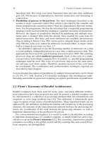
Figure 4.1 illustrates the boundaries for the O-notation, the Ω-notation, and the
Θ-notation according to [31].
The asymptotic running times of global communication operations with respect
to the number of processors in the static interconnection network are given in
Table 4.1. Running times for global communication operations are presented often
in the literature, see, e.g., [100, 75]. The analysis of running times mainly differs
in the assumptions made about the interconnection network. In [75], one-port com-
munication is considered, i.e., a node can send out only one message at a specific
time step along one of its output ports; the communication times are given as func-
tions in closed form depending on the number of processors p and the message
size m for store-and-forward as well as cut-through switching. Here we use the
assumptions given above according to [19].
The analysis uses the duality and hierarchy properties of global communication
operation given in Fig. 3.9 in Sect. 3.5.2. Thus, from the asymptotic running times of
one of the global communication operations it follows that a global communication
operation which is less complex can be solved in no additional time and that a
global communication operation which is more complex cannot be solved faster.
For example, the scatter operation is less expensive than a multi-broadcast on the
same network, but more expensive than a single-broadcast operation. Also a global

communication operation has the same asymptotic time as its dual operation in the
f(n)
c g(n)
c g(n)
c
2
g(n)
c
1
g(n)
n
0
n
0
n
0
nn
n
f(n) = O(g(n)) f(n) = Ω
(g(n))
f(n) = Θ
(g(n))
f(n)
f(n)
Fig. 4.1 Graphic examples of the O-, Ω-, and Θ-notation. As value for n
0
the minimal value
which can be used in the definition is shown
170 4 Performance Analysis of Parallel Programs
Table 4.1 Asymptotic running times of the implementation of global communication operations

depending on the number p of processors in the static network. The linear array has the same
asymptotic times as the ring
Operation Ring Mesh Hypercube
Single-broadcast Θ( p) Θ(
d
√
p) Θ(log p)
Scatter Θ( p) Θ( p) Θ(p/logp)
Multi-broadcast Θ(p) Θ(p) Θ( p/logp)
Total exchange Θ( p
2
) Θ(p
(d+1)/d
) Θ(p)
hierarchy. For example, the asymptotic time derived for a scatter operation can be
used as asymptotic time of the gather operation.
4.3.1.2 Complete Graph
A complete graph has a direct link between every pair of nodes. With the assumption
of bidirectional links and a simultaneous sending and receiving of each output port, a
total exchange can be implemented in one time step. Thus, all other communication
operations such as broadcast, scatter, and gather operations can also be implemented
in one time step and the asymptotic time is Θ(1).
4.3.1.3 Linear Array
A linear array with p nodes is represented by a graph G = (V, E) with a set of
nodes V ={1, ,p} and a set of edges E ={(i, i + 1)|1 ≤ i < p}, i.e., each
node except the first and the final is connected with its left and right neighbors. For
an implementation of a single-broadcast operation, the root processor sends the
message to its left and its right neighbors in the first step; in the next steps each
processor sends the message received from a neighbor in the previous step to its
other neighbor. The number of steps depends on the position of the root processor.

For a root processor at the end of the linear array, the number of steps is p − 1. For
a root processor in the middle of the array, the time is  p/2. Since the diameter of
a linear array is p −1, the implementation cannot be faster and the asymptotic time
Θ(p) results.
A multi-broadcast operation can also be implemented in p −1 time steps using
the following algorithm. In the first step, each node sends its message to both neigh-
bors. In the step k = 2, ,p − 1, each node i with k ≤ i < p sends the message
received in the previous step from its left neighbor to the right neighbor i + 1; this
is the message originating from node i − k + 1. Simultaneously, each node i with
2 ≤ i ≤ p − k + 1
sends the message received in the previous step from its right
neighbor to the left neighbor i −1; this is the message originally coming from node
i + k − 1. Thus, the messages sent to the right make one hop to the right per time
step and the messages sent to the left make one hop to the left in one time step. After
p − 1 steps, all messages are received by all nodes. Figure 4.2 shows a linear array
with four nodes as example; a multi-broadcast operation on this linear array can be
performed in three time steps.
4.3 Asymptotic Times for Global Communication 171
1234
p
p
p
p
21
43
1
2
p
p
p

p
p
p
4
32
3
2
1
12
p
4
3
3
4
p
1
4
step 1
step 2
step 3
Fig. 4.2 Implementation of a multi-broadcast operation in time 3 on a linear array with four nodes
For the scatter operation on a linear array with p nodes, the asymptotic time
Θ(p) results. Since the scatter operation is a specialization of the multi-broadcast
operation it needs at most p − 1 steps, and since the scatter operation is more gen-
eral than a single-broadcast operation, it needs at least p − 1 steps, see also the
hierarchy of global communication operations in Fig. 3.9. When the root node of
the scatter operation is not one of the end nodes of the array, a scatter operation can
be faster. The messages for more distant nodes are sent out earlier from the root
node, i.e., the messages are sent in the reverse order of their distance from the root
node. All other nodes send the messages received in one step from one neighbor to

the other neighbor in the next step.
The number of time steps for a total exchange can be determined by con-
sidering an edge (k, k + 1), 1 ≤ k < p, which separates the linear array into
two subsets with k and p − k nodes. Each node of the subset {1, ,k} sends
p − k messages along this edge to the other subset and each node of the sub-
set {k + 1, , p} sends k messages in the other direction along this link. Thus,
a total exchange needs at least k · (p − k) time steps or p
2
/4fork =p/2.
On the other hand, a total exchange can be implemented by p consecutive scat-
ter operations, which lead to p
2
steps. Altogether, an asymptotic time Θ(p
2
)
results.
4.3.1.4 Ring
A ring topology has the nodes and edges of a linear array and an additional edge
between node 1 and node p. All implementations of global communication opera-
tions are similar to the implementations on the linear array, but take one half of the
time due to this additional link.
A single-broadcast operation is implemented by sending the message from
the root node in both directions in the first step; in the following steps each node
sends the message received in the opposite direction. This results in  p/2 time
steps. Since the diameter of the ring is p/2, the broadcast operation cannot be
implemented faster and the time Θ(p) results.