The boundary element method with programming for engineers and scientists - phần 9 ppsx
Bạn đang xem bản rút gọn của tài liệu. Xem và tải ngay bản đầy đủ của tài liệu tại đây (677.28 KB, 50 trang )
396 The Boundary Element Method with Programming
We discretise the total time into arbitrary small steps of size t' , then we have
(14.34)
where
()
n
Nt
are shape functions in time and
n
u and
n
q are the pressure and pressure
gradient at time step n (at time
n
tnt
'
). If we assume the variation of u and q to be
constant within one time step
t' , then the convolution integrals may be evaluated
analytically. In this case the shape functions are
(14.35)
where H is the Heaviside function. The time interpolation is shown in Figure 14.7.
Substituting (14.34) into (14.33) we obtain the integral equation discretised in time
and written for the time
N
t (time step N):
(14.36)
The convolution integrals are approximated by
(14.37)
and
(14.38)
where
(14.39)
This means that only the fundamental solutions are inside the integrals and these may
be integrated analytically
3
.
The time discretised integral equation now becomes
(14.40)
1
(,, , ) (,) ()
N
NnNn
n
UP Qt qQ q Q U
WW
| '
¦
1
(,, , ) (,) ()
N
NnNn
n
TP Qt uQ u Q T
WW
| '
¦
11
ˆ
() () () () ()
NN
NNnn Nnn
nn
SS
cu P U q Q dS Q T u Q dS Q
''
¦¦
³³
11
(,) () () ; (,) () ()
NN
nn nn
nn
uQt N t u Q qQt N t q Q
¦¦
11
(,, , ) ; (,, , )
nn
nn
tt
Nn N Nn N
tt
UUPQtdTTPQtd
WW WW
' '
³³
1
() ( )
nnn
Nt Htt Htt
ˆ
() [(,,, ) (,) (,,, ) (,)]
NN N
S
cuP UPQt qQ TPQt uQ dS
WWWW
³
DYNAMICS 397
or taking the sum outside the integral
(14.41)
For each time step N we get an integral equation. In a well posed boundary value
problem either u or q is specified on the boundary and the values of u and q are known at
the beginning of the analysis (t=0). Furthermore the integral equation (11.41) must be
satisfied for any source point P. If we ensure the satisfaction at a discrete number of
points P
i
then we can get for each time step N as many equations that are necessary to
compute the unknowns. Similar to static problems we specify the points P
i
to be the
node points of the boundary element mesh (point collocation). To solve the integral
equation we introduce the discretisation in space of Chapter 3:
(14.42)
where
,
nn
uqare pressure and pressure gradients at Q; ,
ee
nj nj
uq refer to values of u and q
at node j of element e at time step n and N
j
are shape functions. Substitution of (14.42)
into (14.41) gives
(14.43)
where
(14.44)
and
(14.45)
J is the Jacobian and E is the number of Elements.
If we define vectors
^`
n
u and
^`
n
q to contain all nodal values of pressure and
pressure gradient at the nodes at time increment N we can rewrite Equation (14.43) in
matrix form
(14.46)
11
ˆ
() () () () ()
NN
NNnn Nnn
nn
SS
cu P U q Q dS Q T u Q dS Q
' '
¦¦
³³
11
( ) ; ( )
JJ
ee
njnjnjnj
jj
uQ N u qQ N q
¦¦
111 111
ˆ
( )
NJ NJ
EE
ee ee
N i ijNn nj ijNn nj
ne j ne j
cu P U q T u
''
¦¦¦ ¦¦¦
()
e
e
ijNn Nn i j
S
UUPNJdS' '
³
()
e
e
ijNn Nn i j
S
TTPNJdS' '
³
>@
^`
>@
^`
11
NN
nn
nn
nn
Tu Uq
¦¦
398 The Boundary Element Method with Programming
If we solve for time step N, the results for the previous time steps are known and can
be put to the right hand side:
(14.47)
or
(14.48)
where the vector
^`
F
contains the effect of the time history. The coefficients of
^`
F
are
(14.49)
14.4 ELASTODYNAMICS
We now turn our attention to general problems in elasticity. The differential equation for
dynamics in the frequency domain can be written in matrix form as:
(14.50)
where
b is a body force vector
(14.51)
and
(14.52)
>@
^`
>@
^`
>@
^`
>@
^`
11
11
NN
NN n n
NN n n
nn
Tu Uq Tu Uq
¦¦
>
@
^`
>
@
^` ^ `
NN
NN
Tu Uq F
11
111 111
NJ NJ
EE
ee
i ijNn nj ijNn nj
ne j ne j
F
Uq Tu
''
¦¦¦ ¦¦¦
2
()GG
OUUZ
uubu
222
2
222
2
222
2
;
x
y
z
x
yxz
x
u
u
y
xyz
y
u
zx zy
z
§·
www
¨¸
ww ww
w
¨¸
§·
¨¸
¨¸
www
¨¸
¨¸
¨¸
ww ww
w
¨¸
¨¸
©¹
www
¨¸
¨¸
ww ww
w
©¹
u
222
222
222
222
222
222
00
00
00
xyz
xyz
x
yz
§·
www
¨¸
www
¨¸
¨¸
www
¨¸
¨¸
www
¨¸
¨¸
www
¨¸
www
©¹
DYNAMICS 399
U
is the mass density and G,
O
are elastic constants introduced in Chapter 4 and
Z
is the
frequency.
The differential equation for dynamics in the time domain can be written in matrix
form as:
(14.53)
where the acceleration vector is defined as
(14.54)
Equation (14.51) can be re-written in terms of pressure and shear velocities,
12
,cc
(14.55)
where
22
12
(2)/ , /cGcG
OU U
.
14.4.1 Fundamental solutions
Fundamental solutions are obtained for a concentrated impulse applied at P at time
W
i.e.
for the case of a body force of
(14.56)
where
G
is the Dirac Delta function introduced earlier.
For 3-D problems the fundamental solution for the displacement is given by:
(14.57)
14.4.2 Boundary integral equations
The integral equation is obtained in a similar way as for the scalar wave equation except
that vectors
u and t are used for the displacements and tractions.
()GG
O
UU
uubu
x
y
z
u
u
u
§·
¨¸
¨¸
¨¸
©¹
u
22 2
12 2
()cc c uubu
()()
j
bPQt
GGW
2
1
,,
,,
22
12
12
1/
,,
1/
1
() ( )
1
(,,,)
4
3()
ij
ij i j
c
ij
ij ij
c
rr
rr
trrt
cc
cc
UP Qt
r
rr t r d
GGG
W
SU
GGOOO
ªº
«»
«»
«»
«»
«»
«»
¬¼
³
400 The Boundary Element Method with Programming
The integral equation is given by
(14.58)
where
U and T are matrices containing the fundamental solutions.
14.4.3 Numerical implementation
For the solution of the integral equation we discretise the problem in time as well as in
space as for the scalar wave equation. If we discretise the total time into equal (arbitrary
small) steps of size
t' then we have
(14.59)
Following the steps for the scalar problem and assuming a constant shape function we
obtain the discretised integral equation for time step N as
(14.60)
where
(14.61)
Introducing the space discretisation
(14.62)
where
,
nn
utare displacements and tractions at Q, ,
ee
nj nj
utrefer to values of u and t at
node j of element e at time step n and
j
N
are shape functions. Substitution of (14.62)
into (14.60) gives
(14.63)
where
(14.64)
ˆ
(,) [(,, ,) (,) (,, ,) (,)]
S
Pt PQt Q PQt Q dS
WWW W
³
cu U t T u
11
(,) () () ; (,) () ()
NN
nn nn
nn
Qt N t Q Qt N t Q
¦¦
uutt
11
ˆ
() () () () ()
NN
NNnn Nnn
nn
SS
P Q dS Q Q dS Q
' '
¦¦
³³
cu U t T u
11
(,,, ) ; (,,, )
nn
nn
tt
Nn N Nn N
tt
PQtd PQtd
WW WW
' '
³³
UU TT
11
( ) ; ( )
JJ
njnjnjnj
jj
QN QN
¦¦
uutt
111 111
ˆ
( )
NJ NJ
EE
ee e e
N i ijNn nj ijNn nj
ne j ne j
P
''
¦¦¦ ¦¦¦
cu U t T u
()
e
e
ijNn Nn i j
S
PN JdS' '
³
UU
DYNAMICS 401
and
(14.65)
where
J
is the Jacobian.
If we define vectors
^`
n
u and
^`
n
t to contain all nodal values of displacements and
tractions at the nodes at time increment N we have
(14.66)
or
(14.67)
where the vector
^`
F contains the effect of the time history:
(14.68)
14.5 MULTIPLE REGIONS
The approach used for the dynamic analysis with multiple regions is very similar to the
one introduced for statics in Chapter 11. The difference is that instead of applying unit
Dirichlet boundary conditions at the interface between regions we apply unit impulses.
We only consider a fully coupled problem to simplify the explanation that we present
here. The details of a partially coupled analysis are given by Pereira et al.
9
Figure 14.8
Example for explaining the analysis of multiple regions
()
e
e
ijNn Nn i j
S
PN JdS' '
³
TT
>@
^`
>@
^`
11
NN
nn
nn
nn
¦¦
Tu Ut
>
@
^`
>
@
^` ^ `
NN
NN
Tu Ut F
11
111 111
NJ NJ
EE
ee
i ijNn nj ijNn nj
ne j ne j
''
¦¦¦ ¦¦¦
FUt Tu
Re
g
ion II
Region I
()ut
402 The Boundary Element Method with Programming
Consider the problem of an inclusion (with different properties) in an infinite domain
in Figure 14.8. We separate the regions and show the displacements and tractions.
Between the regions the conditions of equilibrium and compatibility must be satisfied
(14.69)
where
^` ^`
,
III
ttare interface tractions for region I and II and
^`
0
t are applied tractions.
^` ^`
,
III
uuare the interface displacements. We attempt to derive a relationship between
the tractions and the displacements at the interface between each region.
Figure 14.9 Separated regions
For this we consider each region separately and apply a (transient) unit displacement
at each node while keeping the other displacements zero. We use the concept of the
Duhamel integral introduced earlier to obtain the transient tractions due to transient unit
displacements. If we do this then we obtain the following relationship between tractions
and displacements for region i
(14.70)
where
(, )
i
t
W
K
is a unit displacement impulse response matrix whose coefficients
represent the transient traction components due to an impulsive unit displacement
()t
GW
applied at time
W
. Matrix
(, )
i
t
W
K
can be computed in the Laplace domain using
the CQM introduced above. This is discussed in detail by Pereira
10
.
To solve the fully coupled problem the time may be divided into n time steps
t' .
Then Equation (14.70) may be written for time step n as
(14.71)
^` ^` ^` ^ ` ^ `
0
0 ;
I
II I II
ttt uu
^`
I
t
^`
II
t
^` ^ `
0
() , ()
t
iii
tttd
WW
³
tKu
^` ^`^`
0
0
() (( ))() ()
n
ii
i
m
nt n m t mt mt
ªº
' ' ' '
«»
¬¼
¦
tKut
DYNAMICS 403
where
()
i
nt'K is a “dynamic stiffness matrix” of region i similar to the one obtained in
Chapter 11. Introducing the compatibility and equilibrium equations (14.69) we obtain
the equations for the solution of interface displacements at time
nt'
9
(14.72)
14.6 EXAMPLES
Here we show two examples involving multiple regions. The first is meant to ascertain
the accuracy of the method, the second to show a practical application.
14.6.1 Test example
A standard benchmark example commonly used to validate transient dynamic
formulations is the wave propagation in a rod, as shown in Figure 14.10. The material
properties of the rod are E = 2.1x10
11
N/m
2
,
Q
= 0 and
U
= 7850 kg/m
3
(steel). The road
is divided into two regions. A Heaviside compression load of magnitude 1 kN/m
2
is
applied on the free end of the rod.
Figure 14.10 Step function excitation of a free-fixed steel rod
In the following, all results are normalized by their corresponding static values, i.e.,
the displacements by
s
u 1.4218x10
11
m and the tractions by 1
s
t kN/m
2
, respectively.
The displacements at points
A and B (free end and coupled interface) and the traction in
longitudinal direction at the fixed end are plotted versus time in Figure 14.11 and Figure
14.12, respectively. These results are obtained for different time step sizes. Taking as
reference a parameter
E
= c't / r, where r is the element length, it is possible to identify
^`
^`
^`^`
1
0 0
0
(0) (0) ( )
() (( )) (( ))() ()
III
n
III
m
nt
nt n m t n m t mt mt
'
ªº
' ' ' ' '
¬¼
¦
KK u
tKKut
404 The Boundary Element Method with Programming
a range of values that depend on the time step size where the results are satisfactory i.e.,
stable and accurate. It can be observed, that the results are in good agreement with the
analytic solution and with the numerical results for single region problem published for
example by Schanz
11
. Excellent agreement with the analytic solution is obtained for the
time step
E
= 0.25, however the results for
E
= 0.10 are unstable. The larger time steps
(e.g.,
E
= 1.50) tend to smooth the results due to larger numerical damping and introduce
some phase shift. Nevertheless, the results for all time step sizes inside the interval
0.20<
E
<1.50 are satisfactory.
0
0.5
1
1.5
2
0 0.001 0.002 0.003 0.004 0.005 0.006 0.007 0.008
displacement u
x
/u
s
time [sec]
node A
node B
Analytical:
C= 1.50
C= 1.00
C= 0.50
C= 0.25
C= 0.10
Figure 14.11 Longitudinal normalized displacements at nodes A and B.
Figure 14.12 Longitudinal normalized tractions at the fixed end (node C).
0
0.5
1
1.5
2
0 0.001 0.002 0.003 0.004 0.005 0.006 0.007 0.008
traction t
x
/t
s
time [sec]
node C
Analytical:
C= 1.50
C= 1.00
C= 0.50
C= 0.25
C= 0.10
DYNAMICS 405
14.6.2 Practical application
This is a practical application in tunnelling. The tunnel depicted in Figure 14.13 is
located in a piecewise heterogeneous rock mass with two different properties. The
loading is a suddenly applied point load of magnitude F at the tunnel face.
Figure 14.13 Problem statement
Figure 14.14 Boundary element mesh
406 The Boundary Element Method with Programming
The boundary element mesh consists of 2 regions and linear boundary elements, as
shown in Figure 14.14. Results of the analysis are shown in Figure 14.15, for two
different time steps and values of ratios of Young’s modulus.
Figure 14.15 Contours of absolute displacement for two different ratios of modulus and times
14.7 REFERENCES
1. Banerjee P.K. (1994) The Boundary Element Methods in Engineering, McGraw Hill
Book Company, London.
2. Manolis G.D. and Beskos D.E. (1988) Boundary Element Methods in
Elastodynamics. Unwin-Hyman, London.
3. Dominguez, J. (1993) Boundary Elements in Dynamics. Computational Mechanics
Publications, Southampton.
4. Bonnet, M. (1995) Boundary Integral Equation Methods for Solids and Fluids,
J.Wiley.
5. Chopra A.K. (2007) Dynamics of Structures. Pearson Prentice Hall.
6. Lubich C. (1988) Convolution quadrature and discretized operational calculus I.
Numerische Mathematik.
52: 129-145.
7. Kreyszig, E. (1999) Advanced Engineering Mathematics. J. Wiley
8. Wheeler L.T and Sternberg E. (1968) Some theorems in classical elastodynamics.
Arch. Rational Mech. Anal.
31:51-90.
9. Pereira A. (2006) A Duhamel integral approach based on BEM to 3-D elasto-dynamic
multi-region problems. IABEM, Verlag der TU Graz, Austria, 71-74.
10. Pereira A. (2008) PhD thesis, Graz University of Technology, Austria.
11. Schanz M. (2001) Wave propagation in viscoelastic and poroelastic continua.
Springer, Berlin
15
Nonlinear Problems
SDQWDUHL
(Everything flows)
Aristotle
15.1 INTRODUCTION
So far we have discussed problems where there is a linear relationship between applied
loading and displacement, or between applied flow and temperature/potential. The
system of equations
(15.1)
corresponds to a linear analysis, if {u} is a linear function of {F}.
The linearity of (15.1) is only guaranteed if certain assumptions are made when
deriving the system of equations. These assumptions are:
1. The relationships between flux and temperature/potential or stresses and strains are
linear
2. Matrix
>@
T is not affected by changes in geometry of the boundary that occurs during
loading
3. Boundary conditions do not change during loading
Indeed, we have implicitly relied on these assumptions to be true in all our previous
derivations of the theory.
An example where the first assumption is violated is elasto- or visco-plastic material
behaviour (this is generally referred to as material nonlinear behaviour). The second one
is violated if displacements significantly change the boundary shape (large displacement
problems). Finally, the third no longer holds true for contact problems, where either the
>@
^`^`
FuT
408 The Boundary Element Method with Programming
Dirichlet boundary or the interface conditions between regions change during loading,
thereby affecting the assembly of
>@
T . An example of an elastic sphere on a rigid
surface, shown in Figure 15.1. After deformation two nodes, indicated by dark circles
may change from Neuman to Dirichlet boundary condition.
Figure 15.1 Example of nonlinear analysis: contact problem
If one of the above-mentioned assumptions are not satisfied, then the relationship
between {u} and {F} will become nonlinear. In a nonlinear analysis matrix
>@
T becomes
itself a function of the unknown vector {u}. It is therefore not possible to solve the
system of equations directly.
In this chapter we shall discuss solution methods for nonlinear problems starting with
the general solution process. We will then discuss two different types of nonlinear
behaviour, plasticity and contact problems. We shall see that solution methods for these
types of problems are very similar to the ones employed by the finite element method.
We will also find that the BEM is well suited to deal with contact problems because
boundary tractions are used as primary unknown.
15.2 GENERAL SOLUTION PROCEDURE
The method proposed is to first find a solution with the assumption that the conditions
for linearity are satisfied, i.e. we solve
(15.2)
>
@
^` ^`
0
0
0 Tx F
Original
Deforme
d
409 NONLINEAR PROBLEMS
where
>@
0
T is the “linear” coefficient matrix. With solution vector
^`
0
x (which contains
either displacements or tractions depending on boundary conditions) a check is then
made to see whether all linearity assumptions have been satisfied, for example, we may
check if the internal stresses (computed by post-processing) violate any yield condition,
or if boundary conditions have changed because of deformations. If any one of these
“linearity” conditions has not been satisfied this means that matrix
>@
T has changed
during loading, i.e, instead of equation (15.2) we have
(15.3)
Here
>@
1
T is the changed matrix, also referred to as “tangent” matrix, and
^`
1
R is a
residual vector. Therefore the solution has to be corrected.
We compute the first correction to {x},
^`
x
as
(15.4)
where the overdot means increment and proceed with these corrections until the residual
vector {R} approaches zero.
Final displacements/tractions are obtained by summing all corrections:
(15.5)
where N is the number of iterations to achieve convergence. The solution is assumed to
have converged if the norm of the current residual vector is much smaller than the first
residual vector, i.e., when
(15.6)
where Tol is a specified tolerance.
Alternative to the system of equations (15.4) we may use the “linear” matrix
throughout the iteration, that is, equation (15.4) is modified to
(15.7)
This will obviously result in slower convergence but will save us computing a new
left hand side and a new solution of the system of equations, only a re-solution with a
new right hand side is required. This will be the approach that we will consider here.
^` ^` ^ ` ^ `
01 N
xx x x
"
>
@
^` ^` ^`
01
1
Tx F R
>
@
^` ^`
11
1
Tx R
>
@
^` ^`
11
0
Tx R
Tol
N
d
1
R
R
410 The Boundary Element Method with Programming
15.3 PLASTICITY
There are two ways in which nonlinear material behaviour may be considered: elasto-
plasticity and visco-plasticity
1
. Regardless of the method used, the aim is to obtain initial
strains or stresses. Using the procedures outlined in Chapter 13 residuals {R} may be
computed directly from initial stresses.
15.3.1 Elasto-plasticity
In the theory of elasto-plasticity we define a yield function 0 ),,(
21
CCF
V
which
specifies a limiting value of stress
ı
(C1, C2, etc., are plastic material parameters).
Stress states can only be such that F is negative (elastic states) or zero (plastic states).
Positive values of F are not allowed. Here we restrict the discussion to materials that
exhibit no hardening, although it is clear that the numerical procedures are applicable to
hardening materials also.
Figure 15.2 Mohr-Coulomb yield surface showing elastic and inadmissible stress state
A popular yield function for soil and rock material is the Mohr-Coulomb
2
condition
which can be expressed as a surface in principal stress space by
(15.8)
13 13
() sin cos 0
22
Fc
VV VV
II
ı
V
V
V
n-1)
V
()n
V
'V
V
411 NONLINEAR PROBLEMS
where
31
and
V
V
are maximum and minimum principal stresses, c is cohesion and
I
the
angle of friction. The yield function is plotted as a surface in the principal stress space in
Figure 15.2. We assume that the loading is applied in increments. After the solution it
may occur that stresses that were in an elastic state at a previous load increment n-1 (i.e.
F < 0) change to an inadmissible state (F> 0) at the current increment n (Figure 15.2).
Therefore, this stress state has to be corrected back to the yield surface. To do this we
have to isolate the plastic and elastic components. If the state of stress is such that F(
V
) <
0, then theory of elasticity governs the relationship between stress and strain, i.e. (see
Chapter 4)
(15.9)
For stress states where F(
V
) = 0, elastic strains
H
e
as well as plastic strains
H
p
may be
present, i.e. the total strain , İ , consists of two parts
3
(15.10)
For this case the stress-strain law can only be written incrementally as
(15.11)
where
ep
D is the elasto-plastic constitutive matrix and d
H
is the total strain increment.
To determine
ep
D
we must determine the plastic strain increment. This is
(15.12)
where Q is a flow function whose definition is similar to F. If
QF{ then this is known
as associated flow rule. On the yield surface (F=0) we can write for the stress increment
(15.13)
The stress increment can therefore be split into two parts (one elastic and one plastic)
(15.14)
The condition that
0F ! is not allowed means that for any increment dı the change in F
must be zero, i.e.
(15.15)
ı Dİ
ep
dd ı D İ
ep
İİ İ
p
Q
d
O
w
w
İ
ı
ep
Q
dd dd d
O
w
§·
¨¸
w
©¹
ı D İ D İİ D İ
ı
0
F
d
w
w
ı
ı
ep
dd d ıı ı
412 The Boundary Element Method with Programming
Substitution of (15.13) into (15.15) gives after some algebra
(15.16)
Substituting of (15.16) into (15.13) gives for the plastic stress increment
(15.17)
where
(15.18)
This relationship only holds true if the stress state is actually on the yield surface (
F=0).
In the case where during a load increment a point goes from an elastic to a plastic state
and violates the yield condition in the process (i.e.
F>0) then the plastic stress increment
has to be related to the plastic strain increment rather than the total strain increment.
Figure 15.3 Determination of plastic part of the strain increment
Using a simple linear approximation the plastic strain increment is computed by (Figure
15.3):
(15.19)
where
' has been substituted for d to indicate that the increments are no longer
infinitesimally small and
(15.20)
1
where
T
F
FQ
d
OE
E
www
§·
¨¸
www
©¹
D İ D
ııı
pp
dd ı D İ
1
T
pep
QF
E
ww
§·
¨¸
ww
©¹
DDD D D
ıı
()
() ( 1)
()
()( )
n
nn
F
r
FF
ı
ıı
p
r' 'İİ
H
F ı
F ı
1n
n
p
H
'
H
'
413 NONLINEAR PROBLEMS
Table 15.1 gives an overview of the factor r for different situations of the stress state at
the beginning (n-1) and the end of the load increment (n).
Table 15.1 Values of r for various cases
Case n-1 n r
1 F < 0 F < 0 0.0
2 F < 0 F > 0 Eq. (15.20)
3 F = 0 F > 0 1.0
4 F = 0 F < 0 0.0
After a load increment the stresses have been wrongly computed if they are outside
the yield surface (F>0). They should have to be computed according to
(15.21)
where
(15.22)
Therefore the stresses have to be corrected by
(15.23)
This stress can be assumed as an “initial stress” generated in the domain. Equation
(15.20) is only approximate since a linear variation has been used. Therefore, when
checking the stress state after the correction applied it will not lie exactly on the yield
surface. The discussion of so called “return algorithms” to ensure this are beyond the
scope of this text and the reader is referred to the relevant literature on this subject
4
.
15.3.2 Visco-plasticity
The concept of visco-plasticity allows F(
V
) to be greater than zero
5
. A positive yield
function simply means that the stress state has a higher plastic potential. The stresses are
then allowed to creep back to a lower plastic potential (Figure 15.4) and eventually to the
yield surface. This takes into consideration the fact that the material requires time to
“react” to changes in stress and also allows the consideration of creep behaviour.
The strain rate, at which “creeping” takes place, is assumed to be proportional to the
plastic potential. That is
(15.24)
where
1
()
P
Q
F
t
K
ww
)
ww
H
V
0 p
'ıı
ep
' ' 'ıı ı
pppp
r' ' 'ı D İ D İ
414 The Boundary Element Method with Programming
(15.25)
In the above equations
K
is a material parameter describing its time dependent
behaviour (viscosity).
A visco-plastic analysis proceeds in time steps and a visco-plastic strain increment is
computed at each time step by:
(15.26)
where 't is a time increment. The initial stresses for the computation of the residual are
(15.27)
The time increment 't cannot be chosen freely but has to satisfy certain stability
conditions to prevent oscillations
5
.
Figure 15.4 Explanation of the concept of visco-plasticity
0
00
! )
)
Ffor;F)F(
Ffor;)F(
P
P
t
t
w
' '
w
H
H
0
P
P
' 'ı D
V
H
p
V
'
()n
V
V
n-1)
1
V
2
V
3
V
415 NONLINEAR PROBLEMS
15.3.3 Method of solution
For the solution of problems in plasticity we use a similar method as in Finite Elements
known as the “initial stress” method. In this method we compute initial stresses as
outlined in the previous section and apply this as loading. For this we have to amend the
discretisation of the problem. In addition to surface elements we require the specification
of volume cells in the parts of the domain that are likely to yield, for the integration of
initial stresses. These volume cells have been discussed in Chapter 3. Figure 15.5 shows
examples of discretisations for a cantilever beam and a circular hole in an infinite
domain. The discretisations actually look almost like finite element meshes and it could
be argued that one might as well use finite elements for this problem.
However, there are subtle differences:
x
There is no requirement of continuity, i.e. elements do not need to connect to each
other as finite elements need.
x
There are no additional unknown associated with the mesh of volume cells.
Therefore the system of equations does not increase in size.
x
The representation of stress is still more accurate than with the FEM.
x
The mesh of cells only needs to cover zones where plastic behaviour is expected.
Figure 15.5 Volume cells for the example of a cantilever beam and a circular hole
The iterative process is described in the structure chart in Fig 15.6. First we may
divide the total applied load into increments to optimise the number of iterations. Then
we solve for the unknown displacements/tractions with the applied loading. With the
boundary results we compute the stresses at each cell node and check the yield
condition. If F>0 is detected then the “initial stress” is computed as explained
previously. The residual vector
^`
R is computed as will be explained later and a new
416 The Boundary Element Method with Programming
solution
^
`
m
x
computed and accumulated. The iterations proceed until the norm of the
residual vanishes.
Figure 15.6 Structure chart for plasticity
Determine r,dsxr,Jacobian etc. for kernel computation
Determine distance of Pi to Element, R/L and No. of Gauss points
Load
_
ste
p
: DO i=1,Number of Load ste
p
s
(
cases
)
Iterations: DO m=0, Max. number of iterations
Cells: DO c=1, Number of Cells
Cell_nodes: DO j=1, No. of cell nodes
Initialize
Solve for
^
`
m
x
Calculate ı and ()F ı
() ?F ı
0d
0!
Exit Continue
Calculate
0
ı
Calculate
0
cc
j
ij
'E ı
Calculate
^`
R
? R
Told
Exit Continue
Tol!
Solve for boundary unknowns
^`
0
x
^` ^` ^`
1mm
xx x
417 NONLINEAR PROBLEMS
15.3.4 Calculation of residual {R}
After the initial (linear) analysis the system of equations that has to be solved is
(15.28)
where the components of the residual vector are given by
(15.29)
and
(15.30)
where C is the number of Cells, N is the number of cell nodes and
0
c
n
ı
is the “initial
stress” increment computed at node n of cell c.
The evaluation of integrals
c
ni
'E is similar to the evaluation of
c
ni
'Ȉ , that has been
discussed in section 13.7. For plane problems the expression for
c
ni
'E in intrinsic
coordinates is
(15.31)
Using Gauss Quadrature the formula can be replaced by
(15.32)
where M and K are the number of integration points in
[ and K directions, respectively.
For 3D problems we have
(15.33)
and the integration formula is
(15.34)
11
, (,(,))(,)
MK
c
ni n m k i m k m k m k
mk
N
PQ J WW
[K [K [K
'|
¦¦
Ǽ E
111
111
, , , , ddd
c
ni n i
NPQJ
[
K
]
[K
]
[K
]
[K
]
'
³³³
ǼǼ
111
,, (,(,,))(,,)
LMK
c
ni n m k l i m k l m k l m k l
lmk
N
PQ J WWW
[K] [K] [K]
'|
¦¦¦
Ǽ E
>
@
^` ^ `
Tx R
^`
1
2
§·
¨¸
¨¸
¨¸
©¹
R
RR
#
0
11
CN
cc
inin
cn
'
¦¦
REı
11
11
,,dd
c
c
ni n i n i
V
NPQdV N PQ J
[
K[K[K[K
'
³³³
ǼǼ Ǽ
418 The Boundary Element Method with Programming
with L, M and K being the number of integration points in
[ , K and ] directions.
The matrix
E is given by
(15.35)
with the coefficients
(15.36)
where x,y,z may be substituted for i,j,k and the constants are given in Table 15.2
Table 15.2 Constants for fundamental solution E
Plane strain Plane stress 3-D
n 1 1 2
C
1/8SGQ (1+QSG 1/16SGQ
C
3
1-2
Q (1-QQ 1-2Q
C
4
2
3
The above formulae are valid for the case where none of the cell nodes is the
collocation point. The special case where one of the cell nodes coincides with a
collocation point, P
i
, the kernel
c
ni
'E tends to infinity with o(1/r) for 2-D problems and
o(1/r
2
) for 3-D problems. To evaluate the volume integral for this case we subdivide a
cell into sub cells, as shown in Figure 15.7.
Figure 15.7 Cell subdivision for the case where cell point is a collocation point (plane
problems)
3, , , 4,,,
,
ijk k ij j ik i jk i j k
n
C
EPQ Cr r r Crrr
r
GG G
ªº
¬¼
x
xx xxz
zxx zxz
EE
EE
§·
¨¸
¨¸
¨¸
©¹
E
!
#%#
"
[
K
[
K
Boundar
y
Elemen
t
Subcell
P
i
419 NONLINEAR PROBLEMS
For 2-D problems the subdivision is carried out in exactly the same way as for the
evaluation of the boundary integrals for 3-D problems, i.e., the square domain is mapped
into triangular domains where the apex of the triangle is located at
P
i
(see section 6.3.7).
Equation (15.31) is rewritten as
(15.37)
where
sc is the number of sub-cells, which is equal to 2 if the collocation point P
i
is at a
cell corner node, or 3 if it is a middle node of the cell. The computation of the Jacobian
J
of the transformation from sub element coordinates
K[
,
to intrinsic coordinates
K
[
,
is explained in 6.3.7. Since the Jacobian of this transformation tends to zero with
o(r) as point P
i
is approached, the singularity is cancelled out.
Figure 15.8 Subdivision method for computing singular volume integrals (3-D problems).
For three-dimensional problems, if one of the nodes of the cell is a collocation point,
a subdivision, analogous to the 2-D case, into tetrahedral sub-cells with locally defined
co-ordinate, as shown in Figure 15.8, is used. The integral over the cell is expressed as
(15.38)
11
1
11
111
(,)
( , (, )) (,)
(,)
(,(,)) (, )(, )(, )
sc
c
ni i n
m
sc J
K
i jk njk jk jk jk
mjk
PQ NJ d d
P
QN JJWW
[K
[K [K [ K
[K
[K [K [K [K
w
' |
w
¦
³³
¦¦¦
Ǽ E
E
111
1
111
1111
(,, )
(,(,,)) (,,)
(,, )
(,(,,)) (,,)(,,)
sc
in
m
sc J
KL
i jkl njkl jkl jkl
mjkl
PQ NJ d d d
P
QN JJWWW
[K]
[K] [K] [ K ]
[K]
[K] [K] [K]
w
|
w
¦
³³³
¦¦¦¦
E
E
1
2
3
P
i
[
K
]
1
2
6
5
8
7
3
4
420 The Boundary Element Method with Programming
where
sc is the number of sub-cells which equals to 3 for collocation point at a corner
node, and 4 for collocation point at a mid-node.
J
is the Jacobian of the transformation
from
9
K
[
,,
to
9K[
,, coordinates.
This transformation is given by
(15.39)
Where
l(n) is an array that indicates the local number of node l. For the sub-cell 2 in
Figure 15.8 for example
() (4,1,2,3,8)ln . More details can be found in [6].
The shape functions are defined as
(15.40)
The Jacobian is defined as
(15.41)
where
(15.42)
The Jacobian tends to zero with
o(r
2
) thereby cancelling out the singularity. Having
computed the residual
^`
R
due to an initial stress state
^`
0
ı
we solve the problem for the
boundary unknowns
^
`
x
. The next step is to compute stress increments at the cell and
boundary nodes.
555
() () ()
111
(,, ) ; (,, ) ; (,, )
nln nln n ln
nnn
NNN
[
[K][ K [K]K 9 [K]]
¦¦¦
12
34
5
11
(1 )(1 )(1 ) ; (1 )(1 )(1 )
88
11
(1 )(1 )(1 ) ; (1 )(1 )(1 )
88
1
(1 )
8
NN
NN
N
[
K] [K]
[
K] [K]
[
J
[
K
]
[
[[
[
K
]
K
KK
[
K
]
]]]
www
www
www
www
www
www
5
()
1
( , , ) etc.
n
ln
n
N
[
[K][
[[
w
w
ww
¦