Kinematic Geometry of Surface Machinin Episode 2 pdf
Bạn đang xem bản rút gọn của tài liệu. Xem và tải ngay bản đầy đủ của tài liệu tại đây (2.02 MB, 30 trang )
Preface xix
number of research and application papers and articles. Commonly, isolated
theoretical and practical ndings for a particular surface-generation process
are reported instead of methodology, so the question “What would happen if
the input parameters are altered?” remains unanswered. Therefore, a broad-
based book on the theory of surface generation is needed.
The purpose of this book is twofold:
To summarize the available information on surface generation with a
critical review of previous work, thus helping specialists and prac-
titioners to separate facts from myths. The major problem in the
theory of surface generation is the absence of methods by use of
which the challenging problem of optimal surface generation can be
successfully solved. Other known problems are just consequences of
the absence of the said methods of surface generation.
To present, explain, and exemplify a novel principal concept in the the-
ory of surface generation, namely that the part surface is the primary
element of the part surface-machining operation. The rest of the
elements are the secondary elements of the part surface-machining
operation; thus, all of them can be expressed in terms of the desired
design parameters of the part surface to be machined.
The distinguishing feature of this book is that the practical ways of synthe-
sizing and optimizing the surface-generation process are considered using
just one set of parameters — the design parameters of the part surface to be
machined. The desired design parameters of the part surface to be machined
are known in a research laboratory as well as in a shop oor environment.
This makes this book not just another book on the subject. For the rst time,
the theory of surface generation is presented as a science that really works.
This book is based on the my varied 30 years of experience in research,
practical application,and teaching in the theory ofsurfacegeneration,applied
mathematics and mechanics, fundamentals of CAD/CAM, and engineering
systems theory. Emphasis is placed on the practical application of the results
in everyday practice of part surface machining and cutting-tool design. The
application of these recommendations will increase the competitive posi-
tion of the users through machining economy and productivity. This helps
in designing better cutting tools and processes and in enhancing technical
expertise and levels of technical services.
Intended Audience
Many readers will benet from this book: mechanical and manufacturing
engineers involved in continuous process improvement, research workers
whoareactiveorintendtobecomeactiveintheeld,andseniorundergraduate
and graduate students of mechanical engineering and manufacturing.
© 2008 by Taylor & Francis Group, LLC
xx Preface
This book is intended to be used as a reference book as well as a textbook.
Chapters that cover geometry of sculptured part surfaces and elementary
kinematics of surface generation, and some sections that pertain to design
of the form-cutting tools can be used for graduate study; I have used this
book for graduate study in my lectures at the National Technical University
of Ukraine “Kiev Polytechnic Institute” (Kiev, Ukraine). The design chapters
interest for mechanical and manufacturing engineers and for researchers.
The Organization of This Book
The book is comprised of three parts entitled “Basics,” “Fundamentals,” and
“Application”:
Part I: Basics — This section of the book includes analytical description
of part surfaces, basics on differential geometry of sculptured sur-
faces, as well as principal elements of the theory of multiparametric
motion of a rigid body in E
3
space. The applied coordinate systems
and linear transformations are briey considered. The selected mate-
rial focuses on the solution to the problem of synthesizing optimal
machining of sculptured part surfaces on a multi-axis NC machine.
The chapters and their contents are as follows:
Chapter 1. Part Surfaces: Geometry — The basics of differential
geometry of sculptured part surfaces are explained. The focus
here is on the difference between classical differential geometry
and engineering geometry of surfaces. Numerous examples of the
computation of major surface elements are provided. A feasibility
of classication of surfaces is discussed, and a scientic classica-
tion of local patches of sculptured surfaces is proposed.
Chapter 2. Kinematics of Surface Generation — The general-
ized analysis of kinematics of sculptured surface generation
is presented. Here, a generalized kinematics of instant relative
motion of the cutting tool relative to the work is proposed. For
the purposes of the profound investigation, novel kinds of rela-
tive motions of the cutting tool are discovered, including gen-
erating motion of the cutting tool, motions of orientation, and
relative motions that cause sliding of a surface over itself. The
chapter concludes with a discussion on all feasible kinematic
schemes of surface generation. Several particular issues of kine-
matics of surface generation are discussed as well.
Chapter 3. Applied Coordinate Systems and Linear Transforma-
tions — The denitions and determinations of major applied
coordinate systems are introduced in this chapter. The matrix
© 2008 by Taylor & Francis Group, LLC
and practical implementation of the proposed theory (Part III) will be of
Preface xxi
approach for the coordinate system transformations is briey
discussed. Here, useful notations and practical equations are
provided. Two issues of critical importance are introduced here.
The rst is chains of consequent linear transformations and a
closed loop of consequent coordinate systems transformations.
The impact of the coordinate systems transformations on funda-
mental forms of the surfaces is the second.
These tools, rust covered for many readers (the voice of experience), are
resharpened in an effort to make the book a self-sufcient unit suited for
self-study.
Part II: Fundamentals — Fundamentals of the theory of surface genera-
tion are the core of the book. This part of the book includes a novel
powerful method of analytical description of the geometry of contact
of two smooth, regular surfaces in the rst order of tangency; a novel
kind of mapping of one surface onto another surface; a novel analyti-
cal method of investigation of the cutting-tool geometry; and a set of
analytically described conditions of proper part surface generation. A
solution to the challenging problem of synthesizing optimal surface
machining begins here. The consideration is based on the analytical
results presented in the rst part of the book. The following chapters
are included in this section.
Chapter 4. The Geometry of Contact of Two Smooth Regular Sur-
faces — Local characteristics of contact of two smooth, regular
surfaces that make tangency of the rst order are considered. The
sculptured part surface is one of the contacting surfaces, and the
generating surface of the cutting tool is the second. The performed
analysis includes local relative orientation of the contacting sur-
faces and the rst- and second-order analyses. The concept of
conformity of two smooth, regular surfaces in the rst order of
tangency is introduced and explained in this chapter. For the pur-
poses of analyses, properties of Plücker’s conoid are implemented.
Ultimately, all feasible kinds of contact of the part and of the tool
surfaces
ar
e classied.
Chapter 5. Proling of the Form-Cutting Tools of Optimal Design
— A novel method of proling the form-cutting tools for sculp-
tured surface machining is disclosed in this chapter. The method
is based on the analytical description of the geometry of contact
of surfaces that is developed in the previous chapter. Methods of
proling form-cutting tools for machining part surfaces on con-
ventional machine tools are also considered. These methods are
based on elements of the theory of enveloping surfaces. Numer-
ous particular issues of proling form-cutting tools are discussed
at the end of the chapter.
© 2008 by Taylor & Francis Group, LLC
xxii Preface
Chapter 6. Geometry of Active Part of a Cutting Tool — The gen-
erating body of the form-cutting tool is bounded by the generat-
ing surface of the cutting tool. Methods of transformation of the
generating body of the form-cutting tool into a workable cutting
tool are discussed. In addition to two known methods, one novel
method for this purpose is proposed. Results of the analytical
investigation of the geometry of the active part of cutting tools in
both the Tool-in-Hand system as well as the Tool-in-Use system
are represented. Numerous practical examples of the computa-
tions are also presented.
Chapter 7. Conditions of Proper Part Surface Generation — The
satisfactory conditions necessary and sufcient for proper part
surface machining
ar
e proposed and examined. The conditions
include the optimal workpiece orientation on the worktable of a
multi-axis NC machine and the set of six analytically described
conditions of proper part surface generation. The chapter con-
cludes with the global verication of satisfaction of the condi-
tions of proper part surface generation.
Chapter 8. Accuracy of Surface Generation — Accuracy is an impor-
tant issue for the manufacturer of the machined part surfaces.
Analytical methods for the analysis and computation of the devia-
tionsofthemachinedpart surfacefromthedesiredpartsurfaceare
discussed here. Two principal kinds of deviations of the machined
surface from the nominal part surface
ar
e distinguished. Methods
for the computation of the elementary surface deviations are pro-
posed. The total displacements of the cutting tool with respect to
the part surface are analyzed. Effective methods for the reduction
of the elementary surface deviations are proposed. Conditions
under which the principle of superposition of elementary surface
deviations is applicable are established.
Part III: Application — This section illustrates the capabilities of the
novel and powerful tool for the development of highly efcient
methods of part surface generation. Numerous practical examples of
implementation of the theory are disclosed in this part of the mono-
graph. This section of the book is organized as follows:
Chapter 9. Selection of the Criterion of Optimization — In order to
implement in practice the disclosed Differential Geometry/Kine-
matics (DG/K)-based method of surface generation, an appropri-
ate criterion of efciency of part surface machining is necessary.
This helps answer the question of what we want to obtain when
performing a certain machining operation. Various criteria of ef-
ciency of machining operation are considered. Tight connection
of the economical criteria of optimization with geometrical ana-
logues (as established in Chapter 4) is illustrated. The part surface
© 2008 by Taylor & Francis Group, LLC
Preface xxiii
generation output is expressed in terms of functions of confor-
mity. The last signicantly simplies the synthesizing of optimal
operations of part surface machining.
Chapter 10. Synthesis of Optimal Surface Machining Operations
— The synthesizing of optimal operations of actual part sur-
face machining on both the multi-axis NC machine as well as
on a conventional machine tool are explained. For this purpose,
three steps of analysis are distinguished: local analysis, regional
analysis, and global analysis. A possibility of the development of
the DG/K-based CAD/CAM system for the optimal sculptured
surface machining is shown.
Chapter 11. Examples of Implementation of the DG/K-Based
Method of Surface Generation — This chapter demonstrates
numerous novel methods of surface machining — those devel-
oped on the premises of implementation of the proposed DG/K-
based method surface generation. Addressed are novel methods of
machining sculptured surfaces on a multi-axis NC machine, novel
methods ofmachining surfaces ofrevolution, and a novel method of
nishing involute gears.
The proposed theory of surface generation is oriented on extensive appli-
cation of a multi-axis NC machine of modern design. In particular cases,
implementation of the theory can be useful for machining parts on conven-
tional machine tools.
Stephen P. Radzevich
Sterling Heights, Michigan
© 2008 by Taylor & Francis Group, LLC
Author
Stephen P. Radzevich, Ph.D., is a professor of mechanical engineering and
manufacturing engineering. He has received an M.Sc. (1976), a Ph.D. (1982),
and a Dr.(Eng)Sc. (1991) in mechanical engineering. Radzevich has exten-
sive industrial experience in gear design and manufacture. He has devel-
oped numerous software packages dealing with computer-aided design
(CAD) and computer-aided manufacturing (CAM) of precise gear nishing
for a variety of industrial sponsors. Dr. Radzevich’s main research inter-
est is kinematic geometry of surface generation with a particular focus on
(a) precision gear design, (b) high torque density gear trains, (c) torque share
in multiow gear trains, (d) design of special-purpose gear cutting and n-
ishing tools, (e) design and machining (nishing) of precision gears for low-
noise/noiseless transmissions of cars, light trucks, and so forth. He has spent
more than 30 years developing software, hardware, and other processes for
gear design and optimization. In addition to his work for industry, he trains
engineering students at universities and gear engineers in companies. He
has authored and coauthored 28 monographs, handbooks, and textbooks; he
authored and coauthored more than 250 scientic papers; and he holds more
than 150 patents in the eld. At the beginning of 2004, he joined EATON
Corp. He is a member of several Academies of Sciences around the world.
© 2008 by Taylor & Francis Group, LLC
Acknowledgments
I would like to share the credit for any research success with my numerous
doctoral students with whom I have tested the proposed ideas and applied
them in the industry. The contributions of many friends, colleagues, and
students in overwhelming numbers cannot be acknowledged individually,
and as much as our benefactors have contributed, even though their kind-
ness and help must go unrecorded.
© 2008 by Taylor & Francis Group, LLC
Part I
Basics
© 2008 by Taylor & Francis Group, LLC
3
1
Part Surfaces: Geometry
The generation of part surfaces is one of the major purposes of machin-
ing operations. An enormous variety of parts are manufactured in various
industries. Every part to be machined is bounded with two or more sur-
faces.* Each of the part surfaces is a smooth, regular surface, or it can be
composed with a certain number of patches of smooth, regular surfaces that
are properly linked to each other.
In order to be machined on a numerical control (NC) machine, and for com-
puter-aided design (CAD) and computer-aided manufacturing (CAM) appli-
cations, a formal (analytical) representation of a part surface is the required
prerequisite. Analytical representation of a part surface (the surface P) is
based on analytical representation of surfaces in geometry, specically, (a) in
the differential geometry of surfaces and (b) in the engineering geometry of
surfaces. The second is based on the rst.
For further consideration, it is convenient to briey consider the principal
elements of differential geometry of surfaces that are widely used in this
text. If experienced in differential geometry of surfaces, the following sec-
tion may be skipped. Then, proceed directly to Section 1.2.
1.1 Elements of Differential Geometry of Surfaces
A surface could be uniquely determined by two independent variables.
Therefore, we give a part surface P (Figure 1.1), in most cases, by expressing
its rectangular coordinates X
P
, Y
P
, and Z
P
, as functions of two Gaussian coor-
dinates U
P
and V
P
in a certain closed interval:
r r
P P P P
P P P
P P P
P P P
U V
X U V
Y U V
Z U V
= =
( , )
( , )
( , )
( , )
1
≤ ≤ ≤ ≤; ( ; )
. . . .
U U U V V
P P P P P P1 2 1 2
V
(1.1)
*
The ball of a ball bearing is one of just a few examples of a part surface, which is bounded
with the only surface that is the sphere.
© 2008 by Taylor & Francis Group, LLC
Part Surfaces: Geometry 5
Signicance of the vectors u
P
and v
P
becomes evident from the following
considerations. First, tangent vectors u
P
and v
P
yield an equation of the tan-
gent plane to the surface P at M:
Tangent plane
t p P
M
P
P
⇒
−
( )
r r
u
v
.
( )
1
= 0
(1.3)
where r
t.P
is the position vector of a point of the tangent plane to the surface P
at M, and
r
P
M( )
is the position vector of the point M on the surface P.
Second, tangent vectors yield an equation of the perpendicular N
P
, and of
the unit normal vector n
P
to the surface P at M:
N U V n
N
N
U V
U V
P P P P
P
P
P P
P P
= × = =
×
×
and == ×u v
P P
(1.4)
When the order of multipliers in Equation (1.4) is chosen properly, then the
unit normal vector n
P
is pointed outward of the bodily side of the surface P.
Unit tangent vectors u
P
and v
P
to a surface at a point are of critical impor-
tance when solving practical problems in the eld of surface generation.
Numerous examples, as shown below, prove this statement.
Consider two other important issues concerning part surface geometry —
both relate to intrinsic geometry in differential vicinity of a surface point.
The rst issue is the rst fundamental form of a surface P. The rst funda-
mental form f
1.P
of a smooth, regular surface describes the metric properties
of the surface P. Usually, it is represented as the quadratic form:
φ
1
2 2 2
2
.P P P P P P P P P
ds E dU F dU dV G dV⇒ = + +
(1.5)
where s
P
is the linear element of the surface P (s
P
is equal to the length of a
segment of a certain curve line on the surface P), and E
P
, F
P
, G
P
are funda-
mental magnitudes of the rst order.
Equation (1.5) is known from many advanced sources. In the theory of sur-
face generation, another form of analytical representation of the rst funda-
mental form f
1.P
is proven to be useful:
φ
1
2
0 0
0 0
0 0
0 0 1 0
0 0 0 1
.
[ ]
P P P P
P P
P P
ds dU dV
E F
F G
⇒ = ⋅
⋅
dU
dV
P
P
0
0
(1.6)
© 2008 by Taylor & Francis Group, LLC
6 Kinematic Geometry of Surface Machining
This kind of analytical representation of the rst fundamental form f
1.P
is proposed by Radzevich [10]. The practical advantage of Equation (1.6)
is that it can easily be incorporated into computer programs using mul-
tiple coordinate system transformations, which is vital for CAD/CAM
applications.
For computation of the fundamental magnitudes of the rst order, the fol-
lowing equations can be used:
E F G
P P P P P P P P P
= ⋅ = ⋅ = ⋅U U U V V V, ,
(1.7)
Fundamental magnitudes E
P
, F
P
, and G
P
of the rst order are functions of
U
P
and V
P
parameters of the surface P. In general form, these relationships
can be represented as E
P
= E
P
(U
P
, V
P
), F
P
= F
P
(U
P
, V
P
), and G
P
= G
P
(U
P
, V
P
).
Fundamental magnitudes E
P
and G
P
are always positive (E
P
> 0, G
P
> 0),
and the fundamental magnitude F
P
can equal zero (F
P
≥ 0). This results in the
rst fundamental form always being nonnegative (f
1.P
≥ 0).
The rst fundamental form f
1.P
yields computation of the following major
parameters of geometry of the surface P: (a) length of a curve-line segment
on the surface P, (b) square of the surface P portion that is bounded by a
closed curve on the surface, and (c) angle between any two directions on the
surface P.
The rst fundamental form represents the length of a curve-line seg-
ment, and thus it is always nonnegative — that is, the inequality f
1.P
≥ 0 is
always observed.
The discriminant H
P
of the rst fundamental form f
1.P
can be computed
from the following equation:
H E G F
P P P P
= −
2
(1.8)
It is assumed that the discriminant H
P
is always nonnegative — that is, H
P
= +
E G F
P P P
−
2
.
The fundamental form f
1.P
remains the same while the surface is band-
ing. This is another important feature of the rst fundamental form f
1.P
. The
feature can be employed for designing three-dimensional cam for nishing
a turbine blade with an abrasive strip as a cutting tool.
The second fundamental form of the surface P is another of the two above-
mentioned important issues. The second fundamental form f
2.P
describes
the curvature of a smooth, regular surface P. Usually, it is represented as the
quadratic form
φ
2
2 2
2
.P P P P P P P P P P
d d L dU M dU dV N dV⇒ − ⋅ = + +r n
(1.9)
Equation (1.9) is known from many advanced sources.
© 2008 by Taylor & Francis Group, LLC
Part Surfaces: Geometry 7
In the theory of surface generation, another analytical representation of
the second fundamental form f
2.P
is proven useful:
φ
2
0 0
0 0
0 0
0 0 1 0
0 0 0 1
.
[ ]
P P P
P P
P P
dU dV
L M
M N
⇒ ⋅
⋅
dU
dV
P
P
0
0
(1.10)
This analytical representation of the second fundamental form f
2.P
is pro-
posed by Radzevich [10]. Similar to Equation (1.6), the practical advantage of
Equation (1.10) is that it can be easily incorporated into computer programs
using multiple coordinate system transformations, which is vital for CAD/
CAM applications.
In Equation (1.10), the parameters L
P
, M
P
, N
P
designate fundamental mag-
nitudes of the second order. Fundamental magnitudes of the second order
can be computed from the following equations:
L
U
E G F
M
V
E G
P
P
P
P P
P P P
P
P
P
P P
P P
=
∂
∂
× ⋅
−
=
∂
∂
× ⋅
U
U V
U
U V
2
,
−−
=
∂
∂
× ⋅
−
=
∂
∂
× ⋅
F
U
E G F
N
V
E
P
P
P
P P
P P P
P
P
P
P P
2 2
V
U V
V
U V
,
PP P P
G F−
2
(1.11)
Fundamental magnitudes L
P
, M
P
, N
P
of the second order are also functions
of U
P
and V
P
parameters of the surface P. These relationships in general form
can be represented as L
P
= L
P
(U
P
, V
P
), M
P
= M
P
(U
P
, V
P
), and N
P
= N
P
(U
P
, V
P
).
Discriminant T
P
of the second fundamental form f
2.P
can be computed
from the following equation:
T L N M
P P P P
= −
2
(1.12)
For computation of the principal directions T
1.P
and T
2.P
through a given point
on the surface P, the fundamental magnitudes of the second order L
P
, M
P
, N
P
,
together with the fundamental magnitudes of the rst order E
P
, F
P
, G
P
, are used.
Principal directions T
1.P
and T
2.P
can be computed as roots of the equation
E dU F dV F dU G dV
L dU M dV M dU N dV
P P P P P P P P
P P P P P P P
+ +
+ +
PP
= 0
(1.13)
The rst principal plane section C
1.P
is orthogonal to P at M and passes
through the rst principal direction T
1.P
. The second principal plane section
© 2008 by Taylor & Francis Group, LLC
8 Kinematic Geometry of Surface Machining
C
2.P
is orthogonal to P at M and passes through the second principal direc-
tion T
2.P
.
In the theory of surface generation, it is often preferred to use not the vec-
tors T
1.P
and T
2.P
of the principal directions, but instead to use the unit vectors
t
1.P
and t
2.P
of the principal directions. The unit vectors t
1.P
and t
2.P
are com-
puted from equations t
1.P
= T
1.P
/|T
1.P
| and t
2.P
= T
2.P
/|T
2.P
|, respectively.
The rst R
1.P
and the second R
2.P
principal radii of curvature of the surface
P are measured in the rst and in the second principal plane sections C
1.P
and C
2.P
, correspondingly. For computation of values of the principal radii of
curvature, use the following equation*:
R
E N F M G L
T
R
H
T
P
P P P P P P
P
P
P
P
2
2
0−
− +
+ =
(1.14)
Another two important parameters of local topology of a surface P are (a) mean
curvature
M
P
, and intrinsic (Gaussian or full) curvature
G
P
. These param-
eters can be computed from the following equations:
M
P
P P P P P P P P
P P P
k k E N F M G L
E G F
=
+
=
− +
⋅ −
( )
1 2
2
2
2
2
. .
(1.15)
G
P P P
P P P
P P P
k k
L N M
E G F
= ⋅ =
−
−
1 2
2
2
. .
(1.16)
The formulae for
M
P
k k
P P
=
+
1 2
2
. .
and
G
P P P
k k= ⋅
1 2. .
yield a quadratic equation:
k k
P P P P
2
2 0− + =
M G
(1.17)
with respect to principal curvatures k
1.P
and k
2.P
. The expressions
k k
P P P P P P P P1
2
2
2
. .
= + − = − −
M M G M M G
and
(1.18)
are the solutions to Equation (1.17).
Here, k
1.P
designates the rst principal curvature of the surface P, and k
2.P
des-
ignates the second principal curvature of the surface P at that same point. The
principal curvatures k
1.P
and k
2.P
can be computed from
k R
P P1 1
1
. .
=
−
and k
2.P
=
k
P2.
=
The rst principal curvature k
1.P
always exceeds the second principal curvature
k
2.P
— that is, the inequality k
1.P
> k
2.P
is always observed.
This brief consideration of elements of surface geometry allow for the intro-
duction of two denitions that are of critical importance for further discussion.
Denition 1.1: Sculptured surface P is a smooth, regular surface with
major parameters of local topology that differ when in differential vicin-
ity of any two innitely closed points.
*
Remember that algebraic values of the radii of principal curvature R
1.P
and R
2.P
relate to each
other as R
2.P
> R
1.P
.
© 2008 by Taylor & Francis Group, LLC
Part Surfaces: Geometry 9
It is instructive to point out here that sculptured surface P does not allow slid-
ing “over itself.”
While machining a sculptured surface, the cutting tool rotates about its axis
and moves relative to the sculptured surface P. While rotating with a certain
angular velocity
ω
T
or while performing relative motion of another kind, the
cutting edges of the cutting tool generate a certain surface. We refer to that sur-
face represented by consecutive positions of cutting edges as the generating sur-
face of the cutting tool [11, 13, 14]:
Denition 1.2: The generating surface of a cutting tool can be represented
as the set of consecutive positions of the cutting edges in their motion rela-
tive to the stationary coordinate system, embedded to the cutting tool itself.
In most practical cases, the generating surface T allows sliding over itself. The
enveloping surface to consecutive positions of the surface T that performs
such a motion is congruent to the surface T. When machining a part, the
surface T is conjugate to the sculptured surface P.
Bonnet [1] proved that the specication of the rst and second fundamen-
tal forms determines a unique surface if the Gauss’ characteristic equation
and the Codazzi-Mainardi’s relationships of compatibility are satised, and
those two surfaces that have identical rst and second fundamental forms
are congruent.* Six fundamental magnitudes determine a surface uniquely,
except as to position and orientation in space.
Specication of a surface in terms of the rst and the second fundamental
forms is usually called the natural kind of surface parameterization. In gen-
eral form, it can be represented by a set of two equations:
The natural form
of surface
parameterizatioP nn
⇒ =
=
P P
E F G
P P
P P P P P
P
( , )
( , , )
. .
. .
.
φ φ
φ φ
φ
1 2
1 1
2
==
{
φ
2.
( , , , , , )
P P P P P P P
E F G L M N
(1.19)
Equation (1.19) can be derived from Equation (1.1). Both Equation (1.1) and
Equation (1.19) specify that same surface P. In further consideration, the nat-
ural parameterization of the surface P plays an important role.
Illustrative Example
Consider an example of how an analytical representation of a surface in a
Cartesian coordinate system can be converted into the natural parameteriza-
tion of that same surface [13].
A gear tooth surface G is analytically described in a Cartesian coordinate
system X
g
Y
g
Z
g
(Figure 1.2).
*
Two surfaces with the identical rst and second fundamental forms might also be symmetri-
cal. Refer to the literature—Koenderink, J.J., Solid Shape, The MIT Press, Cambridge, MA, 1990,
p. 699—on differential geometry of surfaces for details about this specic issue.
© 2008 by Taylor & Francis Group, LLC
Part Surfaces: Geometry 11
Substituting the computed vectors U
g
and V
g
into Equation (1.7), one can
come up with formulae for computation of the fundamental magnitudes of
the rst order:
E F
r
G
U r
g g
b g
b g
g
g b g
b g
= = − =
+
1
2 4
2
,
cos
cos
.
.
.
.
τ
τ
and
ccos
.
2
τ
b g
(1.22)
These equations can be substituted directly to Equation (1.5) for the rst
fundamental form:
φ
τ
τ
1
2
2 4
2
.
.
.
.
cos
cos
g g
b g
b g
g g
g b g
dU
r
dU dV
U r
⇒ − +
+
bb g
b g
g
dV
.
.
cos
2
2
2
τ
(1.23)
The computed values of the fundamental magnitudes E
g
, F
g
, and G
g
can be
substituted to Equation (1.6) for f
1.g
. In this way, matrix representation of the
rst fundamental form f
1.g
can be computed. The interested reader may wish
to complete this formulae transformation on his or her own.
The discriminant H
g
of the rst fundamental form of the surface G can be
computed from the formula H
g
= U
g
cosf
b.g
.
In order to derive an equation for the second fundamental form f
2.g
of the
gear-tooth surface G, the second derivatives of r
g
(U
g
, V
g
) with respect to U
g
and V
g
parameters are necessary. The above derived equations for the vectors
U
g
and V
g
yield the following computation:
∂
∂
=
∂
∂
U U
g
P
g
g
U V
0
0
0
1
,
≡
∂
∂
=
V
g
g
b g g
b g g
U
V
V
cos cos
cos sin
.
.
τ
τ
0
1
and
∂
∂
=
− −
− +
V
g
g
b g g g b g g
b g g
V
r V U V
r V
. .
.
cos cos sin
sin
τ
UU V
g b g g
cos cos
.
τ
0
1
(1.24)
Further, substitute these derivatives (see Equation 1.24 and Equation 1.8
into Equation 1.11). After the necessary formulae transformations are com-
plete, then Equation (1.11) casts into the set of formulae for computation of
the second fundamental magnitudes of the surface G is as follows:
L M N U
g g g g b g b g
= = = −0 0 and sin cos
. .
τ τ
(1.25)
After substituting Equation (1.25) into Equation (1.9), an equation for the
computation of the second fundamental form of the surface G can be obtained:
φ τ τ
2
2
. . .
sin cos
g g g g b g b g g
d d U dV⇒ − ⋅ = −r N
(1.26)
© 2008 by Taylor & Francis Group, LLC
12 Kinematic Geometry of Surface Machining
Similar to Equation (1.23), the computed values of the fundamental mag-
nitudes L
g
, M
g
, and N
g
can be substituted into Equation (1.10) for f
2.g
. In this
way, matrix representation of the second fundamental form f
2.g
can be com-
puted. The interested reader may wish to complete this formulae transfor-
mation on his or her own.
Discriminant T
g
of the second fundamental form f
2.g
of the surface G is
equal to
T L M N
g g g g
= − =
2
0
.
The derived set of six equations for computation of the fundamental mag-
nitudes represents the natural parameterization of the surface P:
E
g
= 1
L
g
= 0
F
r
g
b g
b g
= −
.
.
cos
τ
M
g
= 0
G
U r
g
g b g
b g
b g
=
+
2 4
2
2
cos
cos
.
.
.
τ
τ
N U
g g b g b g
= − sin cos
. .
τ τ
All major elements of geometry of the gear-tooth surface can be computed
based on the fundamental magnitudes of the rst f
1.g
and of the second f
2.g
fundamental forms. Location and orientation of the surface G are the two
parameters that remain indenite.
Once a surface is represented in natural form — that is, it is expressed in
terms of six fundamental magnitudes of the rst and of the second order —
then further computation of parameters of the surface P becomes much eas-
ier. In order to demonstrate signicant simplication of the computation of
parameters of the surface P, several useful equations are presented below as
examples.
Examples
1. Length of a curve segment U
P
= U
P
(t), V
P
= V
P
(t), t
0
≤ t ≤ t
1
is given
by
s E
dU
dt
F
dU
dt
dV
dt
G
dV
dt
P P P P
t
=
+ +
2 2
2
00
t
dt
∫
(1.27)
2. Value of the angle q between two given directions through a certain
point M on the surface P can be computed from one of the equations:
cos , sin , tan
θ θ θ
= = =
F
E G
H
E G
H
F
P
P P
P
P P
P
P
(1.28)
© 2008 by Taylor & Francis Group, LLC
Part Surfaces: Geometry 13
3. For computation of square
S
P
of a surface patch S, which is bounded
by a closed line on the surface P, the following equation can be used:
S
P P P P P P
E G F dU dV= −
∫∫
2
S
(1.29)
4. Value of radius of curvature R
P
of the surface P in normal plane
section through M at a given direction can be computed from the
following equation:
R
p
p
P
=
φ
φ
1
2
.
.
(1.30)
5. Euler’s equation for the computation of R
P
is
k k k
P P P
θ
θ θ
. . .
cos sin= +
1
2
2
2
(1.31)
This is also a good illustration of the above statement. (Here q is the angle
that the normal plane section C
P
makes with the rst principal plane section
C
1.P
. In other words,
θ
= ∠( , )
.
t t
P P1
; here t
P
designates the unit tangent vector
within the normal plane section C
P
.)
Shape-index and the curve of the surface are two other useful properties
that are also drawn from the principal curvatures.
The shape-index,
S
P
, is a generalized measure of concavity and convexity.
It can be dened [4] by
S
P
P P
P P
k k
k k
= −
+
−
2
1 2
1 2
π
arctan
. .
. .
(1.32)
The shape-index varies from −1 to +1. It describes the local shape at a
surface point independent of the scale of the surface. A shape-index value
of +1 corresponds to a concave local portion of the surface P for which the
principal directions are unidentied; thus, normal radii of curvature in all
directions are identical. A shape-index of 0 corresponds to a saddle-like local
portion of the surface P with principal curvatures of equal magnitude but
opposite sign.
The curvedness R
P
, is another measure derived from the principal curva-
tures [4]:
R
P
P P
k k
=
+
1
2
2
2
2
. .
(1.33)
© 2008 by Taylor & Francis Group, LLC
14 Kinematic Geometry of Surface Machining
The curvedness describes the scale of the surface P independent of its
shape.
These quantities
S
P
and R
P
are the primary differential properties of the
surface. Note that they are properties of the surface itself and do not depend
upon its parameterization except for a possible change of sign.
In order to get a profound understanding of differential geometry of sur-
faces, the interested reader may wish to go to advanced monographs in the
eld. Systematic discussion of the topic is available from many sources. The
author would like to turn the reader’s attention to the monographs by doCarmo
[2], Eisenhart [3], Struik [16], and others.
1.2 On the Difference between Classical Differential
Geometry and Engineering Geometry
Classical differential geometry is developed mostly for the purpose of inves-
tigation of smooth, regular surfaces. Engineering geometry also deals with
the surfaces. What is the difference between these two geometries?
The difference between classical differential geometry and between engi-
neering geometry is mostly due to how the surfaces are interpreted. Only
phantom surfaces are studied in classical differential geometry. Surfaces of
this kind do not exist in reality. They can be imagined as a thin lm of an
appropriate shape and with zero thickness. Such lm can be accessed from
both of the surface sides. This causes the following indeniteness.
As an example, consider a surface having positive Gaussian curvature
G
P
at a surface point (
G
P
> 0
). Classical differential geometry gives no answer to
the question of whether the surface P is convex (
M
P
> 0
) or concave (
M
P
< 0
)
at this point. In classical differential geometry, the answer to this question can
be given only by convention. A similar observation is made when Gaussian
curvature
G
P
at a certain surface point is negative (
G
P
< 0
).
Surfaces in classical differential geometry strictly follow the equation they
are specied by. No deviation of the surface shape from what is predetermined
by the equation is allowed. More examples can be found in the following chap-
ters of this book.
In turn, surfaces that are treated in engineering geometry bound a part (or
machine element). This part can be called a real object (Figure 1.3). The real
object is the bearer of the surface shape.
Surfaces that bound real objects are accessible from only one side (Figure 1.4).
We refer to this side of the surface as the open side of a surface. The opposite side
of the surface P is not accessible. Because of this, we refer to the opposite side
of the surface P as the closed side of a surface. The positively directed normal unit
vector +n
P
is pointed outward from the part body — that is, from its bodily
side to the void side. The negative normal unit vector −n
P
is pointed opposite
to +n
P
. The existence of open and closed sides of a surface P eliminates the
© 2008 by Taylor & Francis Group, LLC
16 Kinematic Geometry of Surface Machining
selection of appropriate tolerances on shape and dimensions of the actual
surface P
act
easily solve this particular problem.
Similar to measuring deviations, the tolerances are measured in the direc-
tion of the unit normal vector n
P
to the surface P. Positive tolerance d
+
is
measuring along the positive direction of n
P
, and negative tolerance d
−
is
measuring along the negative direction of n
P
. In a particular case, one of the
tolerances, either d
+
or d
−
can be equal to zero.
Often, the value of tolerances d
+
and d
−
are constant within the entire patch
of the surface P. However, in special cases, for example when machining a
sculptured surface on a multi-axis numerical control machine, the actual
value of the tolerances d
+
and d
−
can be set as functions of coordinates of cur-
rent point M on P. This results in the tolerances being represented in terms
of U
P
and V
P
parameters of the surface P, say in the form d
+
= d
+
(U
P
, V
P
) and
d
−
= d
−
(U
P
, V
P
).
The endpoint of the vector d
+
∙ n
P
at a current surface point M produces
point M
+
. Similarly, the endpoint of the vector d
−
∙ n
P
produces the corre-
sponding point M
−
.
The surface P
+
of the upper tolerance is represented by loci of the points
M
+
(i.e., by loci of endpoints of the vector d
+
∙ n
P
). This yields an analytical
representation of the surface of upper tolerance in the form
r r n
P P P P P
U V
+ +
= + ⋅( , )
δ
(1.34)
r
+
P
X
P
P
P
−
r
P
n
P
Y
P
Z
p
P
+
P
act
δ
+
(U
P
,V
P
)
δ
–
(U
P
,V
P
)
M
+
M
–
M
r
–
P
FIGURE 1.5
An example of actual part surface P
act
.
© 2008 by Taylor & Francis Group, LLC
Part Surfaces: Geometry 17
Usually, the surface P
+
of the upper tolerance is located above the nominal
surface P.
Similarly, the surface P
−
of lower tolerance is represented by loci of the
points M
−
(i.e., by the loci of endpoints of the vector d
−
∙ n
P
). This also yields
an analytical representation of the surface of lower tolerance in the form
r r n
P P P P P
U V
− −
= + ⋅( , )
δ
(1.35)
Commonly, the surface P
−
of lower tolerance is located beneath the nominal
surface P.
The actual part surface P
act
cannot be represented analytically.* More-
over, the above-considered parameters of local topology of the surface P
cannot be computed for the surface P
act
. However, because the tolerances
d
+
and d
−
are small compared to the normal radii of curvature of the nomi-
nal surfaces P, it is assumed below that the surface P
act
possesses the same
geometrical properties as the surface P does, and that the difference in
corresponding geometrical parameters of the surfaces P
act
and P is negli-
gibly small. In further consideration, this yields replacement of the actual
surface P
act
with the nominal surface P, which is much more convenient for
performing computations.
The consideration above illustrates the second principal difference between
classical differential geometry and the engineering geometry of surfaces.
Because of the differences, engineering geometry often presents problems
that were not envisioned in classical (pure) differential geometry.
1.3 On the Classification of Surfaces
The number of different surfaces that bound real objects is innitely large. A
systematic consideration of surfaces for the purposes of surface generation is
of critical importance.
1.3.1 Surfaces That Allow Sliding over Themselves
In industry, a small number of surfaces with relatively simple geometry are
in wide use. Surfaces of this kind allow for sliding over themselves. The
property of a surface that allows sliding over itself means that for a certain
*
Actually, surface P
act
is unknown — any surface located within the surfaces of upper tolerance
P
+
and lower tolerance P
−
satises the requirements of the part blueprint; thus, every such
surface can be considered an actual surface P
act
. An equation of the surface P
act
cannot be rep-
resented in the form
P P U V
act act
P P
= ( , )
, because the actual value of deviation δ
act
at the current
surface point is not known. CMM data yields only an approximation for δ
act
as well as the
corresponding approximation for P
act
.
© 2008 by Taylor & Francis Group, LLC
18 Kinematic Geometry of Surface Machining
surface P there exists a corresponding motion of a special kind. When per-
forming this motion, the enveloping surface to the consecutive position of
the moving surface P is congruent to the surface P itself. The motion of the
mentioned kind can be monoparametric, biparametric, or triparametric.
The screw surface of constant pitch (p
x
= Const) is the most general kind
of surface that allows sliding over itself. While performing the screw motion
of that same pitch p
x
, the surface P is sliding over itself, similar to the “bolt-
and-nut” pair.
When the pitch of a screw surface reduces to zero (p
x
= 0), then the screw
surface degenerates to the surface of revolution. Every surface of revolution
is sliding over itself when rotating.
When the pitch of a screw surface rises to an innitely large value, then the
screw surface degenerates into a general cylinder. Surfaces of that kind allow
straight motion along straight generating lines of the surface.
The considered kinds of surface motion are (a) screw motion of constant
pitch (p
x
= Const), (b) rotation, and (c) straight motion, correspondingly. All of
these motions are monoparametric.
Surfaces like that of a circular cylinder allow rotation as well as straight
motion along the axis of the cylinder. In this case, the surface motion is
biparametric (rotation and translation can be performed independently).
A sphere allows for rotations about three axes independently. A plane sur-
face allows straight motion in two different directions as well as a rotation
about an axis that is orthogonal to the plane. The surface motion in the last
two cases (for a sphere and for plane) is triparametric.
Ultimately, one can summarize that surfaces allowing sliding over them-
selves are limited to screw surfaces of constant pitch, cylinders of general
kind, surfaces of revolution, circular cylinders, spheres, and planes. It is
proven [12–15] that there are no other kinds of surfaces that allow for sliding
over themselves.
Surfaces that allow sliding over themselves proved to be very convenient
in manufacturing as well as in industrial applications. Most of the surfaces
being machined in various industries are surfaces of this nature.
1.3.2 Sculptured Surfaces
Many products are designed with aesthetic sculptured surfaces to enhance
their aesthetic appeal, an important factor in customer satisfaction, especially
for automotive and consumer-electronics products. In other cases, prod-
ucts have sculptured surfaces to meet functional requirements. Examples
of functional surfaces can be easily found in aero-, gas- and hydrodynamic
applications (turbine blades), optical (lamp reector) and medical (parts of
anatomical reproduction) applications, manufacturing surfaces (molding
die, die face), and so forth. Functional surfaces interact with the environment
or with other surfaces. Due to this, functional surfaces can also be called
dynamic surfaces.
© 2008 by Taylor & Francis Group, LLC
Part Surfaces: Geometry 19
A functional surface does not possess the property to slide over itself. This
causes signicant complexity in the machining of sculptured surfaces. The
application of a multi-axis NC machine is the only way to efciently machine
sculptured surfaces.
At every instant of surface machining on a multi-axis NC machine, the
sculptured surface being machined and the generating surface of the cut-
ting tool make point contact. In order to develop an advanced technology of
sculptured surface generation, a comprehensive understanding of the local
topology of a sculptured surface is highly desired.
1.3.3 Circular Diagrams
For the purpose of precisely describing the local topology of a surface P,
circular diagrams* can be implemented. Circular diagrams are a powerful
tool for analysis and in-depth understanding of the topology of a sculptured
surface. A circular diagram reects the principal properties of a sculptured
surface in differential vicinity of a surface point.
Euler’s equation for normal surface curvature,
k k k
P P P
θ
θ θ
. . .
cos sin= +
1
2
2
2
(1.36)
together with Germain’s equation (or Bertrand’s equation in other interpretations),
τ θ θ
θ
. . .
( )sin cos
P P P
k k= −
2 1
(1.37)
are the foundation of circular diagrams of a sculptured surface. Here in the
last equation, t
q.P
designates torsion of a surface in the direction specied by
the value of angle q.
Figure 1.6 illustrates an example of a circular diagram constructed for a
convex local patch of the elliptic kind. It is important to point out here that
due to the algebraic value of the rst principal curvature k
1.P
always exceed-
ing the algebraic value of the second principal curvature k
2.P
, the circular dia-
gram point with coordinates (0, k
1.P
) is always located at the far right relative
to the circular diagram point with coordinates (0, k
2.P
).
*
Initially proposed by C.O. Mohr (1835–1918) for the purposes of solving problems in the eld
of strength of materials, circular diagrams later gained wider application. The origination
of application of circular diagrams for the purposes of differential geometry of surfaces can
be traced back to the publications by Miron [7] and Vaisman [17]. Lowe [5,6] applied circular
diagrams in studying surface geometry with special reference to twist, as well as in develop-
ing plate theory. A profound analysis of properties of circular diagrams can be found in pub-
lications by Nutbourn [8] and Nutbourn and Martin [9]. The application of circular diagrams
in the eld of sculptured surface machining on a multi-axis NC machine is known from the
monograph by Radzevich [13].
© 2008 by Taylor & Francis Group, LLC
Part Surfaces: Geometry 21
Finally, the circular diagram of the planar surface local patch (
M
P
= 0
,
G
P
= 0
) is degenerated into the point that coincides with the origin of the
coordinate system k
P
t
P
(Figure 1.7f). All points of plane can be considered as
parabolic umbilics.
As follows from Figure 1.7, the circular diagram clearly illustrates the
major local properties of sculptured surface geometry. Principal curvatures,
normal curvatures, and surface torsion can be easily seen from the diagram.
Moreover, actual values of mean
M
P
and Gaussian
G
P
curvatures can
also be gained from the circular diagram. Figure 1.8 illustrates examples of
how the mean
M
P
and the Gaussian
G
P
curvatures can be constructed.
The examples are given for convex and concave elliptic (Figure 1.7a) local
surface patches, as well as for quasi-convex, and quasi-concave saddle-like
(Figure 1.7a) local surface patches.
The above consideration yields the conclusion that the circular diagram is a
simple characteristic image that provides the researcher with comprehensive
(a)
Concave Elliptic Concave Elliptic
k
1.P
k
2.P
k
1.P
k
2.P
k
P
k
P
k
P
k
P
k
P
k
P
= 0
k
1.P
k
P
G
P
> 0
M
P
< 0
G
P
= 0 M
P
< 0
G
P
< 0 M
P
= 0
G
P
> 0 M
P
> 0
G
P
= 0 M
P
> 0 G
P
< 0 M
P
> 0
G
P
> 0 M
P
< 0 G
P
> 0 M
P
> 0
k
P
< 0 k
P
> 0
G
P
< 0 M
P
< 0
G
P
= 0 M
P
= 0
Convex Umbilic Concave Umbilic
(b)
Convex Parabolic Concave Parabolic
Saddle-Like (pseudoconvex)
Saddle-Like (pseudoconcave)
k
1.P
(c) (d)
Planar
Saddle-Like (minimal)
(e) (f)
τ
P
τ
P
τ
P
τ
P
τ
P
τ
P
k
2.P
k
2.P
k
2.P
k
2.P
k
2.P
k
1.P
k
1.P
k
1.P
FIGURE 1.7
Circular diagrams of smooth, regular local patches of a sculptured surface.
© 2008 by Taylor & Francis Group, LLC
Part Surfaces: Geometry 23
A further shift of the circular diagram in the
V
−
+
direction results in the
consequent change of shape of the local surface patch to a quasi-convex saddle-
like local surface patch, a minimum saddle-like local surface patch, and so
on up to a concave elliptic local surface patch of certain values of principal
curvatures.
Similar changes in shape and in kind of local surface patch are observed
when the circular diagram shifts in the direction of
V
+
−
, which is opposite
to the direction of
V
−
+
.
In order to understand the relationship between the local surface patches
of different kinds, it is convenient to also consider shift of a circular diagram
together with change of ratio between principal curvatures (k
1.P
/k
2.P
) of the
surface. Following this, one can come up with the idea of circular distribu-
tion* of circular diagrams. An example of the circular distribution of the
*
The author would like to credit the idea of circular disposition of local surface patches of
different kinds to J. Koenderink. To the best of the author’s knowledge, Koenderink is the
rst who used circular disposition of images of local surface patches for the purpose of
illustrating the relationship between local surface patches of different geometries. Reading
the monograph by Koenderink [4] inspired the author to apply the circular disposition of
circular diagrams of local surface patches to the needs of kinematical geometry of surface
machining.
k
P
k
P
+
V
−
–
V
+
(a)
(b)
τ
P
τ
P
FIGURE 1.9
Various locations of a circular diagram correspond to local surface patches of different kinds.
© 2008 by Taylor & Francis Group, LLC
24 Kinematic Geometry of Surface Machining
circular diagrams of all possible local patches of a smooth, regular sculp-
tured surface is shown in Figure 1.10.
1.3.4 On Classification of Sculptured Surfaces
Figure 1.10 is helpful for understanding the local topology of the sculp-
tured surface being machined. It also yields classication of local patches of
smooth, regular surface P (Figure 1.11). The classication includes ten kinds
of local surface patches and is an accomplished one.
Based on the analysis of sculptured surface geometry, as well as on the
classication of local surface patches (Figure 1.11), a profound scientic
classication of all feasible kinds of local surface patches is developed by
Radzevich [10]. It is proven that the total number of feasible kinds of local
surface patches is limited. Hence, local surface patches of every kind can be
τ
P
τ
P
�
P
= 0
C
C
C
C
C
C
C
k
P
< 0
k
P
= 0
C
k
P
> 0
CC
C
C
k
P
C
C
C
C
k
P
C
C
< 0
= 0
= 0
< 0
= 0
< 0
= 0
< 0
< 0
< 0
< 0
< 0
> 0
< 0
> 0
< 0
> 0
= 0
< 0
= 0
> 0
= 0
< 0
> 0
> 0
> 0
> 0
> 0
= 0
< 0
= 0
< 0
= 0
= 0
< 0
FIGURE 1.10
Smooth, regular local patches of a sculptured surface: relationship between local patches of
various kinds.
© 2008 by Taylor & Francis Group, LLC