Plastics Engineering 3E Episode 7 pot
Bạn đang xem bản rút gọn của tài liệu. Xem và tải ngay bản đầy đủ của tài liệu tại đây (1.36 MB, 35 trang )
194
Mechanical Behaviour
of
Composites
when the stresses
a,, ay
and
txy
are applied. Calculate also the strains in the
global
X
-
Y
directions.
E1
=
125O0O1
MN/m2,
E2
=
7800
MN/m2,
u12
=
0.34
a,
=
10
MN/m2,
ay
=
-14
MN/m2,
txy
=
-5
MN/m2
Solution
The Stress Transformation Matrix
is
G12
=
4400
MN/m2,
c2
s2
2sc
0.671 0.329 0.94
)
T,
=
[
s2
c2
-2sc
]
or
T,
=
(
0.329 0.671 -0.94
-sc
sc
(2
-
2)
-0.47 0.47 0.342
The stresses parallel and perpendicular to the fibres are then given by
[E:]
=To.
[
21
t12
=xY
so,
a1
=
-2.59
MN/m2
02
=
-1.4
MN/m2
t12
=
-12.98
MN/m2
In order to get the strains in the global directions it is necessary to determine
the overall compliance matrix
[SI.
This is obtained as indicated above, ie
[SI
=
[a]-'
where
[a]
=
[To]-'
[e].
[T,]
The local compliance matrix is
-
0
0
1
-
and
Q=S-'
The Strain Transformation matrix
is
c2
s2
SC
-2sc
2sc
(2
-2)
T,
=
[
s2
c2
-sc
]
-
so,
Q=T;'.Q.T,
and
s=a-'
Then
6.64
x
-2.16
x
-7.02
x
["]=3.["]
-
s
=
[
-2.16
x
10-~
1.07
x
10-~
-4.27
x
10-~
YXY
TXY
-7.02
x
10-~
-4.27
x
10-~ 1.51
x
10-~
Mechanical Behaviour
of
Composites 195
Directly by matrix manipulation
E,
=
1.318
x
lod3
cy
=
-1.509
x
yxy
=
8.626
x
or by multiplying out the
terms
E,
=
[(s11).
(a,)
+
(512)
(ay)]
+
(516).
(txy)
E,
=
1.318
x
and similarly for the other
two
strains.
3.8
General Deformation Behaviour of a Single
Ply
The previous section
has
considered the in-plane deformations of a single ply.
In
practice, real engineering components are likely to be subjected to
this
type
of loading plus (or
as
an alternative) bending deformations. It is convenient
at
this
stage to consider the flexural loading of a single ply because
this
will
develop the method of solution for multi-ply laminates.
(i)
Loading
on
Fibre Axis
Consider
a
unidirectional sheet
of
material with the fibres aligned in the
x-
direction and subjected to a stress,
u,.
If the sheet has thickness,
h,
as shown
in Fig. 3.15 and we consider unit width, then the normal axial force
N,
is
given by
!!
2
N,
=
/ox&
h
2
_-
Fig.
3.15
General
forces
and
moments acting
on
a
single
ply
196
Mechanical Behaviour of Composites
Or more generally for all the force components
N,,
N,
and
N,,
h
2
[NI
=
JI.1.
h
2
_-
Similarly the bending moment,
MI,
per unit width is given by
h
-2
Once again, all the moments
M,,
My
and
M,,,
can
be
expressed
as
h
2
[MI
=
/[alzdz
-2
h
(3.27)
(3.28)
Now in order to determine
[a]
as
a function of
z,
consider the strain
E(Z)
at
any depth across
the
section. It will be made up of an in-plane component
(E)
plus a bending component
(z/R)
which is normally written
as
Z.K,
where
K
is
the curvature of bending.
Hence,
The stresses will then
be
given by
E(Z)
=
E
-k
Z.K
dz)
=
[Ql
*
[&I
+
[Ql
*
Z.[K]
where
[Q]
is the stiffness matrix
as
defined earlier.
Now, from equation
(3.27),
the forces
[N]
are
given by
VI
=
[AI[&]
+
[Bl[Kl
(3.29)
where
[A]
is the
Extensional Stiffness
matrix
(=
[Qlh)
and
[B]
is a
Coupling
Matrix.
It may
be
observed that in the above analysis
[B]
is in fact zero for
Mechanical Behaviour of Composites
197
this
simple single ply situation. However, its identity has been
retained
as
it
has relevance in laminate analysis, to
be
studied later.
Returning to equation
(3.28),
the
moments may
be
written
as
h h
[MI
=
[Bl[~l+
PI[KI
(3.30)
where
[D]
is the Bending Stiffness Matrix
(=
[Q]h3/12).
Equations
(3.29)
and
(3.30)
may
be
grouped into
the
following form
[E]
=
[:
4
[:I
(3.31)
and these are known
as
the
Plate Constitutive Equations.
the strains by
For
this
special case of a single ply,
[B]
=
0
and
so
the forces
are
related
to
[NI
=
[AI[&]
(3.32)
(which
is
effectively
[a]
=
[Q][E]
as
shown previously) or the strains are related
to
the forces by
[E]
=
[a][N]
where
[a]
=
[A]-'
(which is effectively
[E]
=
[S][a]
as
shown previously).
by
Also, for the single ply situation, the moments are related to the curvature
[MI
=
[DI[Kl
(3.33)
or
the curvature is related to the moments by
[K]
=
[d][M]
where
[d]
=
[D]-'
It should
be
noted that it is only possible to utilise
[a]
=
[AI-'
and
[dl
=
[DI-'
for the special case where
[B]
=
0.
In other cases, the terms in the
[a]
and
[d]
matrices have to
be
determined from
A B
-'
[i
:I=[,
D]
(3.34)
198
Mechanical Behaviour of Composites
(ii)
Loading
off
Fibre
Axis
For
the
situation where the loading
is
applied off the fibre axis, then the
above approach involving the Plate Constitutive Equations can
be
used but it
is necessary to use the
transformed
stiffness matrix terms
0.
Hence, in the above analysis
[AI
=
@I
*
h
103
=
@I.
h3/12
The use
of
the Plate Constitutive Equations
is
illustrated in the following
Examples.
Example
3.9
For the
2
mm
thick unidirectional carbon fibre/PEEK
composite described in Example
3.6,
calculate the values of the moduli,
Poisson’s Ratio and strains in the global direction when a
stress
of
a,
=
50
MN/m2 is applied. You should use
(i) the lamina stiffness and compliance matrix approach and
(ii) the Plate Constitutive Equation approach.
Solution
(i)
As
shown in Example
3.6,
for
the
loading in Fig.
3.16
I
4.12
10-~
-2.58
x
10-~
-6.24
x
10-~
-2.58
x
lo-’
7.87
x
1.77
x
lo-’
m2h4N
-6.24
10-5
1.77
10-5
1.43
10-4
yk
n
I
’/
0
Fig.
3.16
Single
ply
composite subjected
to
plane
stress
Mechanical Behaviour
of
Composites
199
and
1 1
s11
522
Ex
=
=-
=
24.26
GN/m2,
E,
=
=-
=
12.7
GN/m2
1
2
Gxy
=
=
6.9
GN/m
,
vxy
=
-Ex??21
=
0.627
s66
vYx
=
-EyS12
=
0.328
Also,
Ex
=
2.06
x
ly
=
-1.29
=
-3.12 10-~
Note that
As
cry
=
0
in
this
Example
vxy
=
E'
=
0.627
as above
EX
(ii) Alternatively using the Plate Constitutive Equation Approach.
N,
=
oxh
=
100
N/m,
N,
=
0,
Nxy
=
0.
A=
D=
4.86
x
104 3.76
x
104 1.65
x
104
N/mm
2.06
x
16
4.86
x
lo4
8.37
x
104
8.37
x
104 1.65
x
104 4.84
x
lo4
1.62
x
lo4
1.25
x
104
5.51
x
16
N
mm
6.86
x
lo4
1.62
x
104 2.79
x
lo4
1
1
2.79
x
io4
5.51
x
io3
1.61
x
io4
a
=
A-'
and
d
=
D-'
(since
B
=
0)
-1.29
x
3.93
x
8.89
x
mm/N
-3.12
x
8.89
x
7.16
x
1
2.06 10-~ -1.29
x
10-~ -3.12
x
10-~
200
Mechanical Behaviour of Composites
-a12
v,,
=
-,
1
6.18
x
10-~ -3.87
x
104
9.37
x
104
-3.87
x
1.18
x
2.66
x
(N
mm)-’
-9.37
x
10-5 2.66
x
10-5 2.14
x
10-4
a22
x
h’ wxh’
a1
1
1 1
1
E,
=
-
G,,
=
-
E,
=
-
all
x h’
-a12
vp
=
-
a22
E,
=
24.26
GN/m2,
E,
=
12.7
GN/m2
Gxy
=
6.98
GN/m2,
vxy
=
0.627,
up
=
0.328
These values agree with those calculated above. Also, for the applied force
N,
=
50
x
2
=
100
N/mm.
[5]
=a.
[;?I
(=a[;]
-”)
E,
=
2.061
x
cy
=
-1.291
x
yxy
=
-3.124
x
It
is interesting to observe that
as
well
as
the expected axial and transverse
strains arising
from
the applied axial stress,
a,,
we have
also
a shear strain.
This is because in composites we can often get
coupling
between the different
modes
of
deformation.
This
will also be seen later where coupling between
axial and flexural deformations can occur in unsymmetric laminates. Fig.
3.17
illustrates why the shear strains arise in uniaxially stressed single ply in
this
Example.
Orlginal
unidirectional
composite
Deformed
shape
Fig.
3.17
Coupling
effects
between extension and
shear
Mechanical Behaviour of Composites
20 1
Example
3.10
If a moment
of
My
=
100
Nm/m is applied to the unidirec-
tional composite described in
the
previous Example, calculate the curvatures
which will occur. Determine also the stress and strain distributions in the global
(x-y)
and local
(1-2)
directions.
Solution
Using the
D
and
d
matrices from the previous Example, then for
the applied moment
My
=
100 N:
This enables the curvatures to be determined as
K~
=
-3.87
m-',
K~
=
12 m-',
K~~
=
2.67 m-',
vYX
=
0.328,
vXY
=
3.05
The bending strains in the global directions are given generally by
E
=
K.Z
Hence
(&y)max
=
f
Ky
(f)
=
f
0.012
(Yxy)max
=
f
Kxy
(f)
=
f
2.67
x
The stresses are then obtained from
so
a,
=
0,
ay
=
150 MN/m2.
tXy
=
0
For the local directions, the strain and stress transformation matrices can
be used:
[
=To.
[
"1
t12
TXY
so
cq
=
26.8 MN/m2,
a2
=
123.2 MN/m2,
txv
=
57.5 MN/m2
202
Mechanical Behaviour of Composites
[":I
=Tea
[
:]
Y12 YXY
so
~1
=
-5.14
x
~2
=
8
x
y12
=
0.014
These stresses and strains are illustrated in Fig. 3.18.
Global strains Global stresses
0
0.39% -1.2%
0
-0.27%0
0
-150
0
0
-0.39%
0
0
1.2%
0
0.27%
0
0
150
0
v
7
Y
(3
EX
CY
rv
0,
Local strains Local
stresses
0
-0.8%
0
-1.4%
0
-26.80 -123
0
-57.5
0
0
0.8%
0
1.4%
0
26.8
0
123
0
57.5
0
712
€1
€2
r12
01
(32
Fig.
3.18
Stresses
and
strains,
Example
3.10
Note that if both plane stresses and moments are applied then the total
stresses will be the algebraic sum of the individual stresses.
3.9
Deformation Behaviour of Laminates
(i) Laminates Made from Unidirectional Plies
The previous analysis has shown that the properties of unidirectional fibre
composites
are
highly anisotropic.
To
alleviate this problem, it is common to
build up laminates consisting of stacks of unidirectional lamina arranged at
different orientations. Clearly many permutations are possible in terms of the
numbers of layers (or plies) and the relative orientation of the fibres in each
Mechanical Behaviour of Composites
203
layer. At first glance it might appear that the best means
of
achieving a more
isotropic behaviour would be to have two layers with the unidirectional fibres
arranged perpendicular to each other. For example, two layers arranged at
0"
and 90" to the global x-direction or at
+45"
and -45" to the x-direction might
appear to offer more balanced properties in all directions. In fact the lack of
symmetry about the centre plane of the laminate causes very complex behaviour
in such cases.
In general it is best to aim for symmetry about the centre plane.
A
lami-
nate in which the layers above the centre plane are a mirror image
of
those
below it is described
as
symmetric. Thus a four stack laminate with fibres
oriented at
0",
90", 90" and
0"
is symmetric. The convention is
to
denote this
as [oo/900/900/o"]T or
[0",
90;, Oo]T or [0"/90"],. In general terms any laminate
of the type
[e,
-8,
-8,
e]T
is symmetric and there may
of
course be any even
number of layers
or
plies. They do not all have to be the same thickness but
symmetry must be maintained. In the case of a symmetric laminate where the
central ply is not repeated, this can be denoted by the use of an overbar. Thus
the laminate
[45/
-
45/0/90/0/
-
45/45]T can be written
as
[f45,0,
%lS.
In-plane Behaviour
of
a
Symmetric
Laminate
The in-plane stiffness behaviour of symmetric laminates may
be
analysed as
follows. The plies in a laminate
are
all securely bonded together
so
that when
the laminate is subjected to a force in the plane of the laminate, all the plies
deform by the same amount. Hence, the strain is the same in every ply but
because the modulus of each ply is different, the stresses are not the same. This
is illustrated in Fig.
3.19.
Fig.
3.19
Stresses
and
strains in
a
symmetric
laminate
When external forces
are
applied
in
the global
x-y
direction, they will equate
to the summation of all the forces in the individual plies. Thus, for unit width
where
h
is the thickness
of
the laminate.
a,,
N,
are the overall stresses
or
forces
and
(a)f
is the stress in the ply
'f'
(see Fig.
3.20).
f
th
layer
hl2
L-
Fig.
3.20
Ply
f
in
the
laminate
In matrix form we can write
Mechanical Behaviour
of
Composites
205
As
the strains are independent of
2
they can be taken outside the integral:
where, for example,
A11
=
TalldZ
=
2.
-h/2
0
[A]
is the
Extensional Stiffness Matrix
although it should be noted that it also
contains shear terms.
Within a single ply, such as the fth, the
e
-
terms are constant
so,
In
overall terms
P
[AI
=
CDhf
f
=I
(3.35)
Thus the stiffness matrix for a symmetric laminate may be obtained by
adding, in proportion to the ply thickness, the corresponding terms in the stiff-
ness matrix for each of the plies.
Having obtained all the terms for the extensional stiffness matrix
[A],
this
may then be inverted to give the compliance matrix
[a].
[a]
=
[AI-'
The laminate properties may then be obtained as above from inspection
of
the compliance matrix.
1
G=-
1
1
Ex
=
-
E,
=
-
allh
.
a22h a66h
where
h
is the thickness of the laminate.
-a12 a12
Vyx
=
-
a11 a22
vx,
=
-
206
Mechanical Behaviour
of
Composites
3.10
Summary
of
Steps
to Predict Stiffness
of
Symmetric Laminates
1. The Stiffness matrix
[GI
is obtained
as
earlier each individual ply in the
laminate.
2.
The Stiffness matrix
[A]
for the laminate
is
determined by adding the
product of thickness and
[GI
for each ply.
3.
The Compliance matrix
[a]
for the laminate is determined
by
inverting
[A]
ie
[a]
=
[AI-'.
4.
The stresses and strains in the laminate are then determined from
{~}=~a~.{
:}h
YXY
TXY
Example
3.11
A
series of individual plies with the properties listed below
are laid in the following sequence to make a laminate
Determine the moduli for the laminate in the global
X-Y
directions and the
strains
in
the laminate when stresses of
a,
=
10 MN/m2,
cy
=
-
14
MNlm2
and
tXy
=
-5
MN/m2 are applied. The thickness
of
each is
1
mm.
E1
=
125000
MN/m2
E2
=
7800
MN/m2
G12
=
4400
MN/m2
~12
=
0.34
Solution
The behaviour
of
each ply when subjected to loading at
13
degrees
off
the fibre axis is determined using Matrix manipulation
as
follows:
Compliance Matrix StifSness Matrix
Stress Transformation Matrix Strain Transformation Matrix
c2
s2
2sc sc
-sc
sc
(2
-
s2)
s2
c2
-2sc
]
Mechanical Behaviour
of
Composites
207
Overall Stiffness Matrix
Overall Compliance Matrix
-
Q(0)
=
T,'
.
Q.
T,
S(e)
=
Q(e)-I
6.27
io4
2.71
io4
3.66 io4
2.71
x
IO4
2.21
x
IO4
1.87
x
IO4
3.66
x
io4
1.87
io4
2.88
io4
Hence, the Extension Stiffness matrix
is
given by
A
=
2.Q(O)
+
4.e(35)
+
4.Q(-35)
A
=
2 22
x
105
1.93
x
105
[7:530,
105
2.22 105
]Nmm
0
2.39
x
IO5
The compliance matrix is obtained by inverting [A]
I
a
=A-
u
=
-2.31
x
lop6
7.84
x
lop6
[
2.0
;IOp6
-2.31
x
lop6
0
]
(Nmm-I)
0
4.17
x
lop6
The stiffness terms in the global directions may be obtained
from:
1
E,
=
E,
=
49.7
GN/m2
all
x
IO'
1
1
E,
=
E,
=
12.8
GN/m2 and
G,,
=
=
24
GN/III~
a22
x
10'
a66
x
10
(note the high value
of
Poisson's Ratio which can be obtained in composite
laminates)
vyx
=
0.295
a12
uyx
=
-
a22
and the strains may be obtained as
E,
[;J
=a.
[;I
E,
=
5.24
sy
=
1.33
x
yxy
=
-2.08 lop4
E,
=
0.052%,
E,
=
-0.133%,
rry
=
-0.021%
It may be seen from the above analysis that for cross-ply
(0/90),
and symmetric
angle ply [-O/O], laminates,
A16
=
,461
=
0
and
A26
=
A62
=
0
(also
a16
=
a61
=
a62
=
0).
For other types
of
laminates this will not be the case.
208
Mechanical Behaviour
of
Composites
3.1
1
General Deformation Behaviour
of
Laminates
The previous section has illustrated a simple convenient means
of
analysing
in-plane loading
of
symmetric laminates. Many laminates
are
of
this
type and
so
this approach is justified. However, there
are
also many situations where
other types
of
loading (including bending) are applied to laminates which may
be symmetric or non-symmetric. In order to deal with these situations it is
necessary to adopt a more general type
of
analysis.
Convention
for
defining
thicknesses and positions
of
plies
In this more general analysis it is essential to be able to define the position and
thickness
of
each ply within a laminate. The convention is that the geometrical
mid-plane is taken as the datum. The top and bottom
of
each ply are then defined
relative to
this. Those above the mid-plane will have negative co-ordinates and
those below will be positive. The bottom surface
of the fth ply has address
hf
and the top surface
of this
ply has address
hf-1.
Hence the thickness
of
the
fth ply is given by
h(f)
=
hf
-
hf-1
For the
6
ply laminate shown in Fig.
3.21,
the thickness
of
ply
5
is given by
h(5)
=
hs
-h4
=
3
-
1
=
2
mm
Fig.
3.21
Six
ply
laminate
The thickness
of
ply
1
is given by
h(1)
=
hl
-
h~
=
(-3)
-
(-6)
=
3
mm
Mechanical Behaviour of Composites
209
Analysis
of
Laminates
The general deformation analysis of a laminate is very similar to the general
deformation analysis for a single ply.
(i)
Force
Equilibrium:
If there are
F
plies, then the force resultant,
NL,
for
the laminate is given by the sum of the forces for each ply.
F F
hf
[NIL
=
CWIf
=
/
[Olfdz
hf-i
f
=I
f
=1
and using the definition for
[a]
from the analysis of a single ply,
F
[NIL.
=
E(@]
.
[&I
f
=I
[el
.
Z
.
[Kl)fdz
where
(3.36)
(3.37)
This is called the
Extensional StifSness Matrix
and the similarity with that
derived earlier for the single ply should be noted.
Also, the
Coupling
Matrix,
[B]
is
given by
(3.38)
The Coupling Matrix will be zero for a symmetrical laminate.
(ii)
Moment Equilibrium:
As in the case of the forces, the moments may be
summed across
F
plies to give
F
F
hf
[MIL
=
C[MIf
=
/
[UlfdZ
hf-1
f
=I
f
=I
210 Mechanical Behaviour of Composites
and once again using the expressions
from
the analysis
of
a single ply,
F
hf
[MIL
=
J
([QI[&lZ
+
[al[Klz2)dz
hf-1
f=1
[MIL
=
[BI[EIL
+
[DI[K]L
(3.39)
where
[B]
is as defined above and
(3.40)
As
earlier we may group equations (3.36) and (3.39) to give the
Plate Consti-
lF
[Dl
=
3
C[iZIf
ch;
-
f=1
tutive Eauation
as
[;I
=
[;
:]
[:I
(3.41)
This
equation may
be
utilised to give elastic properties, strains, curvatures, etc.
It
is much more general than the approach in the previous section and can
accommodate bending as well as plane stresses. Its use
is
illustrated in the
following Examples.
Example
3.12
For the laminate [0/352/
-
3521, determine the elastic
constants in the global directions using the Plate Constitutive Equation.
When stresses of
a,
=
10
MN/m2,
u
-
-14 MN/m2 and
txy
=
-5
MN/m2
y
are applied, calculate the stresses and strams in each ply in the local and global
directions.
If
a moment of
M,
=
lo00
N
m/m is added, determine the new
stresses, strains and curvatures in the laminate. The plies
are
each
1
mm
thick.
El
=
125 GN/m2,
E2
=
7.8
GN/m2, G12
=
4.4 GN/m2,
u12
=
0.34
Solution
The locations of each ply are illustrated in Fig. 3.22.
Using the definitions given above, and the
values for each ply, we may
determine the matrices
A,
B and
D
from
10
A=
CiZf(hf -hf-l),
f=1
Mechanical Behaviour
of
Composites
21
1
Fig.
3.22
Ten
ply
laminate
Then
EX
NX
[;;I
=a.
[;;I
=a.
[3
*h
where
h
=
full laminate thickness
=
10
mm,
and
a
=
A-’
since
[B]
=
0.
This
matrix equation gives the global strains
as
Ex
=
5.24
=
1.33
x
eXy
=
2.08
10-~
Also,
1
Gxy
=
-
1
E,
=
-
all
*
h’
a22
-
h’
a66.h
-a12
-a12
Vxy
=
-
,
up=-
all
a22
E,
=
12.8 GN/m2,
1
E,
=
-
E,
=
49.7 GN/m2,
Gxy
=
24 GN/m2
uXy
=
1.149
U~
=
0.296
It
may
be
seen that these values agree with those calculated in the previous
Example.
To
get
the
stresses
in the global (xy) directions
for
the
‘f’th
ply
when
f
=
1,
f
=2,
f
=9
and
f
=
10
ax
=
4.5
MN/m2,
a,
=
-11.3
MN/m2,
txy
=
-0.28
MNlm2
212
Mechanical Behaviour of Composites
when
f
=3,
f
=4,
f
=7 and
f
=
8
a,
=
-10.8 MNIm’,
a,
=
-19.2 MNlm2,
txy
=
-11.8 MNlm2
when
f
=5and6
a,
=
62.6
MNlm2,
a,,
=
-9
MNlm2,
txy
=
-0.9
MNIm’.
Note that in the original question, the applied force per unit width in the
x-direction was
100
Nlmm (ie
a,
(10)).
As
each ply is 1
mm
thick, then the
above stresses are also equal to the forces per unit width for each ply.
If
we
add the above values for all 10 plies, then it will be seen that the answer is
100 Nlmm as it should be for equilibrium. Similarly, if we add
N,
and
N,,
for
each ply, these come to -140
Nlmm
and
-50
Nlmm which also agree with
the applied forces in these directions.
In the local (1
-2)
directions we can obtain the stresses and strains by using
the transformation matrices. Hence, for the tf’th ply
[
::I
=
T,
[
;]
[E:]
=TEf
[
21
t12
T*Y
Y12
YXY
So
that for
f
=
1,
2, 9
and 10
a1
=
-0.44
MNlm2,
a2
=
-6.4 MNlm2,
txy
=
7.3 MNlm2
c1
=
1.38
x
g2
=
-8.15
x
y12
=
1.67
10-~
For
f
=
3,4,7 and
8
01
=
-0.96 MN/m2,
a2
=
-5.8
MN/m2,
q2
=
-7.5 MNlm2
=
1.82
E2
=
-6.2
x
y12
=
-1.8
10-~
For
f
=5and6
a1
=
4.5
MNIm’,
a2
=
-11.3 MNlm2, t12
=
-0.28
MN/m2
g1
=
5.25
x
g2
=
-1.33
x
y12
=
-2.09
10-~
When the moment
M,
=
10o0 Ndm is added, the curvatures,
K,
can be
calculated from
Mechanical Behaviour of Composites 213
where
d
=
D-'
since
[B]
=
0.
K~
=
0.435 m-',
K~
=
-0.457 m-',
K~~
=
-0.147 m-l
uXy
=
1.052
uYx
=
0.95
When the bending moment is applied the global stresses and strains in each
ply may be obtained as follows:
E,
=
Kx
.
z,
Ey
=
Ky
.
z,
yxy
=
Kxy
.
z
At the top surface,
Z
=
-5 mm
=
-2.17
x
=
2.28
yxy
=
-7.34
x
10-~
and the stresses are given by
So
that
a,
=
-47 MN/m2,
uy
=
5.7 MN/m2,
rxy
=
15.4 MN/m2.
The local stresses and strains are then obtained from the stress and strain
transformations
[
5'2
TXY
Y12
YXY
u2
=
2.8 MN/m2,
=
T,,
[
"1
and
[
]
=
T,,
[
"1
u1
=
-44.1 MN/m2,
ti2
=
-19.5
MN/m2
=
-3.6
E2
=
4.7
x
y12
=
-4.44
x
10-~
For the next interface,
z
=
-4
mm,
the new values of
E~,
and
yxy
can be
calculated and hence the stresses in the global and local co-ordinates.
f
=
1
and
f
=
2
need to be analysed for this interface but there will
be
continuity
across the interface because the orientation of the plies is the same in both
cases. However, at
z
=
-3 mm there will be a discontinuity of stresses in the
global direction and discontinuity of stresses and strains in the local directions
due to the difference in fibre orientation in plies 2 and 3.
The overall distribution of stresses and strains in the local and global direc-
tions is shown in Fig. 3.23. If both the normal stress and the bending are applied
together then it is necessary to add the effects of each separate condition. That
is, direct superposition can
be
used to determine the overall stresses.
214
Mechanical Behaviour of Composites
Global
strains
Global
stresses
4.2%
0
0
0.23%
4
07%
0
-47
0 0
57 -19.50
0
02%423%
0
0
0.07%
0
47
-57
0
0
19.5
._
. .
_
€1
€2
'y12
01
02
712
(b)
Fig.
3.23
Stresses
and
strains,
Example 3.12:
(a)
global;
(b)
local
Note, to assist the reader the values of the terms in the matrices are
A
=
2.22
x
105 1.93
x
16
17.52; 105 2.22
x
105
000
x
IN/-
B=
0 0
0
[o
0
01
0
2.39
x
105
[
2.01;
lo6
-2.31
x
u
=
-2.31
x
7.82
x
0
]
(N/mm)-'
0
4.17
x
2.24
x
lo6
1.84
x
lo6
-9.042
x
lo5
Nmm,
5.25
x
lo6
2.24
x
lo6
-1.75
x
lo6
-1.75
x
lo6
-9.04
x
16 2.38
x
lo6
1
1
D=
[
4.34
x
10-~ -4.57
x
10-~ 1.46
x
10-~
1.46
x
10-~ 9.75
x
io-8
5.63
x
10-~
-4.57
x
1.14
x
9.75
x
(NIIMI)-'
The solution method using the Plate Constitutive Equation is therefore
straightforward and very powerful. Generally a computer is needed to handle
Mechanical Behaviour of Composites
215
the matrix manipulation
-
although this is not difficult, it is quite time-
consuming if it has to be done manually.
The following Example compares the behaviour of a single ply and a
laminate.
Example
3.13
A
single
ply
of carbon fibre/epoxy composite has the
following properties:
El
=
175 GN/m2,
E2
=
12
GN/m2, G12
=
5
GN/m2,
u12
=
0.3
Plot the variations of E,,
E,,
G,, and
uxy
for values of
8
in the range
0
to
90"
for (i) a single ply
0.4
mm thick and (ii) a laminate with the stacking sequence
[4=8],.
This
laminate has four plies, each
0.1
mm
thick.
Discuss
the meaning
of the results.
Solution
(i)
Single
ply
The method of solution simply involves the determination of
[SI, [el, [el,
[SI
and
[a]
as illustrated previously, ie
PI
=
Then
1
0
0-
GI2
=
T,
.
Q
.
T,
and
and
IAl
=
le1
.
h
Then for
8
=
25"
(for example)
=
28.3
GN/m2
1
E,
=
-
allh
-
11.7 GN/m2
1
a22h
1
Q66h
E
Y-
G,,
=
-
=
7.3 GN/m2
a12
-a1
I
uxy
=
-
- -
0.495
and
a12
a22
u,,
=
-
=
0.205
Fig.
3.24
shows
the
variation of these elastic constants for all values of
8
between
0
and
90".
216
180
160
140
120
E
2
100
s2.
-
2
80
N
Lo
40
20
0
Mechanical Behaviour of Composites
0
10
20
30
40
50
60
70
80
90
Angle
(e)
Fig.
3.24
Variation
of
elastic properties
for
a
single ply
of
carbodepoxy composite
(ii) Symmetric
4
Ply Laminate The same procedure
is
used
again except that
this time the
IAl
matrix has to
be
summed for all the plies, ie
f=4
f=1
IAl
=
IZilf
(hf
-
hf-1)
and
la1
=
1AI-l
where
l~
=
-0.2,
hl
=
-0.1,
h2
=
0,
h3
=
O.l,h4
=
0.2.
Once again, for
8
=
50"
(for example)
E,
=
-
=
14.6
GN/m2
1
Ullh
ad
E
-
24.8
GN/m2
Y-
1
Gxy
=
-
=
44
GN/m2
a66h
-a12
-
1.045
VXY
=
-
=0.615
and
vYx=
-a12
a1
1
a22
Fig.
3.25
shows the variation of these elastic constants for values of
8
in the
range
0
to
90".
Mechanical Behaviour of Composites
217
180
160
140
40
20
0
01020~405060708090
Angle
(e)
Fig.
3.25
Variation
of
elastic properties
for
a
(+/
-
45)
symmetric
laminate
of
carbodepoxy
It is interesting to compare the behaviour of the single ply and the laminate
as shown in Figs
3.24
and
3.25.
Firstly it is immediately evident that the lami-
nate offers a better balance of properties
as
well
as
improvements in absolute
terms. The shear modulus in particular is much better in the laminate. Its peak
value at
45"
arises because shear is equivalent to a state of stress where equal
tensile and compressive stresses are applied at
45"
to the shear direction. Thus
shear loading on a
[&
451,
laminate is equivalent to tensile and compressive
loading on a
[0/90],
laminate. Thus the fibres are effectively aligned in the
direction of loading and this provides the large stiffness (or modulus) which is
observed.
It is also worthy of note that large values of Poisson's Ratio can occur
in a laminate. In this case a peak value of over
1.5
is observed
-
something
which would be impossible in an isotropic material. Large values of Poisson's
Ratio are a characteristic of unidirectional fibre composites and arise due to the
coupling effects between extension and shear which were referred to earlier.
It
is
also important to note that although the laminae
[It
451,
indicates that
Ex
=
E,
=
18.1
GN/m2, this laminate
is
not isotropic
or
even quasi-isotropic.
As
shown in Chapter
2,
in an isotropic material, the shear modulus
is
linked
to the other elastic properties by the following equation
218
Mechanical Behaviour of Composites
For
the
[&
451,
laminate this would give
18.1
G-
=
5
GN/m2
xy
-
2(1
+
0.814)
However, Fig.
3.25
shows that
G,,
=
45.2
GN/m2 for the
[f
45Is
laminate.
Some laminates do exhibit quasi-isotropic behaviour. The simplest one is
[0,
f
601,.
For this laminate
E,
=
E,
=
66.4
GN/m
If
we check
Gxy
from the isotropic equation we get
2
and
uxy
=
uyx
=
0.321,
Gxy
=
25.1
GN/m2
(using the individual ply data in the above Example).
=
25.1
GN/m2
66.4
Ex
-
-
2(1+
uxy)
2(1
+
0.321)
Gxy
=
This agrees with the value calculated
from
the laminate theory.
In general any laminate with the lay-up
or
is quasi-isotropic where
N
is an integer equal to
3
or greater. The angles for
the plies are expressed in radians.
3.12
Analysis
of
Multi-layer Isotropic Materials
The Plate Constitutive equations can be used for curved plates provided the
radius of curvature
is
large relative to the thickness (typically
r/h
>
50).
They
can also
be
used to analyse laminates made up of materials other than unidi-
rectional fibres, eg layers which are isotropic or made from woven fabrics can
be
analysed by inserting the relevant properties for the local
1-2
directions.
Sandwich panels can also
be
analysed by using a thickness and appropriate
properties for the core material. These types of situation are considered in the
following Examples.
Example
3.14
A
blow moulded plastic bottle
has
its wall thickness made
of
three
layers. The layers are:
Outside and inside
skin
-
Material
A
thickness
=
0.4
mm,
El
=
E2
=
3
GN/m2,
Gl2
=
1.1
GN/m2,
u12
=
0.364
Core
-
Material
B
thickness
=
0.4
mm,
E1
=
E2
=
0.8
GN/m2,
Glz
=
0.285
GN/m2,
1112
=
0.404.