Báo cáo y học: " Factor correction as a tool to eliminate between-session variation in replicate experiments: application to molecular biology and retrovirology" ppsx
Bạn đang xem bản rút gọn của tài liệu. Xem và tải ngay bản đầy đủ của tài liệu tại đây (291.87 KB, 8 trang )
BioMed Central
Page 1 of 8
(page number not for citation purposes)
Retrovirology
Open Access
Research
Factor correction as a tool to eliminate between-session variation
in replicate experiments: application to molecular biology and
retrovirology
Jan M Ruijter*
1
, Helene H Thygesen
2
, Onard JLM Schoneveld
3,4
, Atze T Das
5
,
Ben Berkhout
5
and Wouter H Lamers
3,1
Address:
1
Department of Anatomy and Embryology, Academic Medical Centre, Meibergdreef 15, 1105 AZ Amsterdam, The Netherlands,
2
Department of Clinical Epidemiology and Biostatistics, Meibergdreef 15, 1105 AZ Amsterdam, The Netherlands,
3
AMC Liver Center, University
of Amsterdam, Meibergdreef 69-71, 1105 BK, Amsterdam, The Netherlands,
4
Laboratory of Signal Transduction, National Institute of
Environmental Health Sciences, National Institutes of Health, Research Triangle Park, NC, USA and
5
Department of Human Retrovirology,
Academic Medical Centre, Meibergdreef 15, 1105 AZ Amsterdam, The Netherlands
Email: Jan M Ruijter* - ; Helene H Thygesen - ;
Onard JLM Schoneveld - ; Atze T Das - ; Ben Berkhout - ;
Wouter H Lamers -
* Corresponding author
Abstract
Background: In experimental biology, including retrovirology and molecular biology, replicate
measurement sessions very often show similar proportional differences between experimental conditions,
but different absolute values, even though the measurements were presumably carried out under identical
circumstances. Although statistical programs enable the analysis of condition effects despite this replication
error, this approach is hardly ever used for this purpose. On the contrary, most researchers deal with
such between-session variation by normalisation or standardisation of the data. In normalisation all values
in a session are divided by the observed value of the 'control' condition, whereas in standardisation, the
sessions' means and standard deviations are used to correct the data. Normalisation, however, adds
variation because the control value is not without error, while standardisation is biased if the data set is
incomplete.
Results: In most cases, between-session variation is multiplicative and can, therefore, be removed by
division of the data in each session with a session-specific correction factor. Assuming one level of
multiplicative between-session error, unbiased session factors can be calculated from all available data
through the generation of a between-session ratio matrix. Alternatively, these factors can be estimated
with a maximum likelihood approach. The effectiveness of this correction method, dubbed "factor
correction", is demonstrated with examples from the field of molecular biology and retrovirology.
Especially when not all conditions are included in every measurement session, factor correction results in
smaller residual error than normalisation and standardisation and therefore allows the detection of smaller
treatment differences. Factor correction was implemented into an easy-to-use computer program that is
available on request at: ?subject=factor.
Conclusion: Factor correction is an effective and efficient way to deal with between-session variation in
multi-session experiments.
Published: 06 January 2006
Retrovirology 2006, 3:2 doi:10.1186/1742-4690-3-2
Received: 21 December 2005
Accepted: 06 January 2006
This article is available from: />© 2006 Ruijter et al; licensee BioMed Central Ltd.
This is an Open Access article distributed under the terms of the Creative Commons Attribution License ( />),
which permits unrestricted use, distribution, and reproduction in any medium, provided the original work is properly cited.
Retrovirology 2006, 3:2 />Page 2 of 8
(page number not for citation purposes)
Background
In experimental biology, including retrovirology and
molecular biology, replicating a series of measurements
under presumably identical circumstances often leads to
results that show the same proportional differences
between experimental conditions, but very different abso-
lute values within each of the conditions. As an example
Figure 1A shows data from a multi-session experiment in
which multiple promoter-luciferase-reporter constructs
were transfected into hepatoma cells. Luciferase activity
was quantified two days after transfection [1]. Although
the different constructs demonstrate a similar pattern of
luciferase activity in each of the sessions, the activity for
some of the constructs can vary up to 30-fold in different
sessions. This between-session variation results from
small, but systematic, differences in e.g. cell density, sub-
strate and reagent concentration, reaction temperature
and exposure time, which all can be shown to proportion-
ally increase or decrease the outcome of all biological
measurements in a session [2]. The between-session vari-
ation can therefore be modelled as a multiplicative factor
working on the data in each session. As exemplified in Fig-
ure 1A, the between-session variation can be very large
and may conceal differences between the activities of the
different constructs. A pair-wise comparison of each of the
DNA constructs with construct 1 indeed revealed no sta-
tistically significant differences in the measured data (Fig.
2A; t-test, all P > 0.4). One way to test whether the activity
of constructs differs despite this confounding between-
session variation is to apply analysis of variance
(ANOVA). However, even though this method is available
in statistical programs, ANOVA is hardly ever used for this
purpose in biochemistry, virology or molecular biology
because these programs are elaborate and hard to use for
the non-expert. In practice, most researchers use their own
'normalisation' method, which is often not validated and
seldom mentioned in the methods section of the paper.
The importance of using good and reliable statistical
methods was recently discussed in detail for the field of
virology [3] but obviously holds for all disciplines of
experimental biology and medicine [4]. However, in these
papers the handling of this between-session variation is
not discussed. The current paper intends to bridge the gap
between statistical theory and laboratory practice with
respect to the removal of between-session variation.
The most popular methods used to remove between-ses-
sion variation in bio-medical research are "normalisa-
tion" and "standardisation" [5]. In normalisation, a
"control" condition is defined and per session all meas-
ured values (Y
ni
) are divided by the control value in the
session (Eq. 1, with session n, condition i and control
condition 1).
Thus a single control condition is chosen to serve as a cor-
rection factor (100/Y
n1
in Eq. 1). Figure 1B shows the data
from Figure 1A when normalisation, using DNA construct
1 as control, is applied. Since DNA construct 1 was lost in
one session (᭜) normalisation led to the loss of this entire
session. Normalisation does remove some between-ses-
sion variation but because the control condition itself car-
ries biological error, this can lead to an increased
variation. The variation for constructs 6 and 8, i.e., is
much larger after normalisation compared to the original
data (compare Figs. 2A and 2B). Another drawback of nor-
malisation is that it generates a control condition without
normalised Y 100
Y
Y
Eq
ni
ni
n1
=×
()
.1
Comparison of normalisation, standardisation and factor cor-rectionFigure 1
Comparison of normalisation, standardisation and
factor correction. DNA constructs containing different
enhancer, promoter, and intron sequences from the rat
glutamine synthetase gene coupled to the firefly luciferase
reporter gene were transfected into FTO-2B cells. Luciferase
activity was measured 64 hours after transfection [1]. This
plot shows the activity of 8 different DNA constructs (= con-
ditions) measured in 6 independent measurement sessions
(᭜ ᮀ ▲ ●). A: Original measurements, plotted on a
logarithmic Y-axis. The approximately parallel lines connect-
ing the results from each session indicate that most of the
variation between the sessions is multiplicative. B: Data after
normalisation, using condition 1 as 'control' (one session [᭜]
did not include condition 1 and had to be dropped). Note
that the variation in the control condition ('c') is lost. C: Data
after standardisation. Note that a linear transformation of
the standardised values (standardised* = 410 + 305 × stand-
ardised) was required to enable this logarithmic plot. D: Data
after applying factor correction. The minimal remaining dis-
tance between the lines indicates that factor correction is
most effective in removing the multiplicative between-ses-
sion variation.
Retrovirology 2006, 3:2 />Page 3 of 8
(page number not for citation purposes)
variation. Since parametric statistical tests for the compar-
ison of two or more conditions assume an equal variance
in all conditions [6] these tests can no longer be used. Also
most nonparametric tests are no longer applicable,
because they require similar distributions in all condi-
tions [7].
In standardisation [5], each value per session is trans-
formed into a standard value by subtracting the session
mean ( ) and dividing the result by the session standard
deviation (SD
n
, Eq. 2).
Because the session mean after standardisation becomes
zero for each session, standardisation removes between-
session variation (Fig. 1C). However, the original meas-
urement scale is lost and the overall mean becomes zero.
Furthermore, if not all conditions are present in every ses-
sion, the session mean and standard deviation will be
biased. Because the standard deviation serves as multipli-
cative correction factor, this bias can result in added vari-
ability between sessions (as observed for the sessions
indicated with triangles and filled diamonds in Fig. 1C).
Standardisation can, therefore, only be used effectively
when the data set is complete, that is, when all conditions
are present in every session.
As mentioned above, the between session variation is due
to multiplicative session factors. When known, these fac-
tors can be used to correct the data. As was demonstrated
in the previous paragraphs, normalisation and standardi-
sation both use correction factors that can lead to ineffec-
tive correction or even to an increased variation within
conditions. For a correction method to be effective, the
correction factors should be based on all available obser-
vations in the session and the estimation of these factors
should not be affected by incomplete data sets. This paper
describes such a correction method, dubbed "factor cor-
rection" and introduces two approaches to estimate cor-
rection factors. In the first, "ratio", approach the variation
in the data set is assumed to be restricted to the condition
effects whereas in the second, "maximum likelihood"
approach part of the variation may result from variation
among the factors affecting the individual measurement
in each session. Both approaches turn out to result in very
similar correction factors. Their use and effectiveness are
illustrated using data sets from molecular biology and ret-
rovirology.
Results
Mixed additive and multiplicative model
In the molecular-biology data set plotted in Figure 1A, the
different DNA constructs represent the experimental con-
ditions. Data from transfection experiments carried out
on different days are the measurement sessions. The mul-
tiplicative nature of the between-session variation in this
data set is apparent from the fact that the lines connecting
the data points in each session run approximately parallel
in a logarithmic plot of the data (Fig. 1A). In a multi-ses-
sion experiment with such a multiplicative between-ses-
sion variation, the observations can be described with a
mixed additive and multiplicative model (Eq. 3).
Y
ni
= F
n
× (Y
mean
+ E
i
+ error
ni
) (Eq. 3)
The additive part of this model, between parenthesis,
states that the result of a measurement Y in condition i is
the sum of the population mean (Y
mean
), the effect of con-
dition i (E
i
), and an experimental error. Note that 'effect'
in the sense used here does not represent the difference
between a control and an experimental condition, but
stands for the effect of each condition relative to the pop-
ulation mean. Therefore, the sum of the condition effects
Y
n
standardised Y
YY
SD
Eq
ni
ni n
n
=
−
()
.2
Comparison of normalisation, standardisation and factor cor-rectionFigure 2
Comparison of normalisation, standardisation and
factor correction. Mean (and SEM) of the data of the
molecular-biology data set from Figure 1 A: original data. B:
normalised data. C: standardised data. D: data after factor
correction. Note that normalisation, standardisation, and fac-
tor correction reduce the variation within each condition.
However, normalisation (B) leads to loss of variance in the
control condition ('c') and to added variation in the other
conditions. Standardisation (C) of this incomplete data set
leads to increased variation, compared to factor correction,
in some conditions. With factor correction (D) all conditions
retain their statistical variance, which is generally smaller
than after normalisation and standardisation. An asterisk indi-
cates a statistically significant difference between the DNA
construct and construct 1 (t-test; P < 0.05). Note that the
number of observations per construct in these comparisons
ranges from 2 to 5.
Retrovirology 2006, 3:2 />Page 4 of 8
(page number not for citation purposes)
is 0 ( ). In this model the biological error is nor-
mally distributed with mean 0 and standard deviation
σ
.
This biological error reflects the variance within a condi-
tion, whereas the condition effects reflect the differences
between conditions [6]. For each session n, the additive
part of the observation is multiplied by session factor F
n
.
The product of the session factors equals 1 ( ),
which insures that the mean of Y
ni
is still equal to the over-
all Y
mean
.
The session factors can be estimated from all available
data in the multi-session data set with two different
approaches: calculation of a between-session ratio matrix
(Ratio approach) or a maximum likelihood approach.
Estimation of the session factors with the Ratio approach
To estimate the session factors with the Ratio approach for
each pair of sessions, a between-session ratio is calculated
(Eq. 4). For e.g. session 5 and 6, and condition i, this ratio
is:
In such a between-session ratio, the normally distributed
additive parts of the multi-session model (Y
mean
+ E
i
+
error
ni
), have the same mean and standard deviation, and
hence a ratio of 1. The error of such a ratio of normally dis-
tributed variables has a Cauchy distribution [8], which
implies that, strictly speaking, its mean does not exist.
However, the Cauchy distribution has a symmetrical clock
shape centred on zero, has a median of zero [8] and, with
a more general definition of integration, its mean can also
be considered to be zero [9]. Therefore, on average, the
error in the last term of Eq. 4 is zero and the term cancels
out which makes the between-session ratio an unbiased
estimate of the ratio of two session factors. When two ses-
sions have more than one condition in common, a
between-session ratio is calculated for each matching pair
of conditions. Because we are dealing with multiplicative
effects, the geometric mean of these ratios [10] is used in
the between-session ratio matrix.
In the example data set (Fig. 1A), sessions 1 and session 6
have no conditions in common and, therefore, a between-
session ratio cannot be directly calculated for this pair of
sessions. To be able to calculate proper session factors
without the loss of data sets like sessions 1 and 6, missing
between-session ratios have to be substituted. It is possi-
ble to calculate a substitution for a missing ratio in col-
umn j and row i (R
j/i
) from a known ratio in that column
(e.g. R
j/n
) and two other ratios from these two rows in
another column (R
k/i
and R
k/n
). A substitute value for the
missing ratio R
j/i
is then calculated as R
j/i
= R
j/n
× R
k/i
/R
k/n
.
If such a substitute is computed for all possible R
j/n
, R
k/i
,
and R
k/n
the geometric mean of all values will be the best
estimate of the missing ratio R
j/i
.
Because the product of all session factors in the multi-ses-
sion model equals 1, the geometric mean of column i in
this between-session ratio matrix is an estimate of the cor-
rection factor for session i:
The between-session variation in the original data set can
now be removed by dividing each measured value by the
corresponding session factor (Eq. 6):
The corrected data are shown in Fig. 1D.
Estimation of session factors with the maximum likelihood
approach
In the above mixed additive and multiplicative model the
error term is normally distributed with a standard devia-
tion
σ
. When we define =
σ
·F
n
and = Y
i
/
σ
with Y
i
as
the mean value per condition (Y
i
= Y
mean
+ E
i
; see Eq. 3)
the model can be rewritten as Y
ni
= ( + error
ni
/
σ
), and
can then be shown to be normally distributed
with mean 0 and standard deviation 1. Based on this form
of the model, the likelihood of the observed set of Y
ni
is
given by Eq. 7
which is the chance of finding each individual observa-
tion Y
ni
given F
n
and Y
i
, multiplied (Π) for all observa-
tions.
If this likelihood function is maximal for = Y
i,max
, =
F
n,max
, then Y
i,max
and F
n,max
are found when the first deriv-
atives in Y and F of the log of this likelihood function
equal 0. The estimation equations for Y
i
and F
n
are not
E
i
i
I
=
=
∑
0
1
F
n
n
N
=
=
∏
1
1
between-sessionratio
Y
Y
F
F
Y E error
Y
6i
5i
6
5
mean i ni
me
65/
()
(
==×
++
aan i ni
E error
Eq
++
()
)
.4
geometric meancolumn
F
F
F
F
FEq
i
i
j
j=1
n
n
i
n
j
j=1
n
n
i
=
=
()
=
∏
∏
5
()
corrected Y
Y
F
Eq
ni
ni
n
=
()
.6
F
n
’
Y
i
’
F
n
’
Y
i
’
Y
F
Y
ni
n
i
’
’
−
Le
Y
F
Y
ni
n
i
=
()
−−
∏
1
2
7
1
2
2
π
()
’
.Eq
Y
i
’
F
n
’
Retrovirology 2006, 3:2 />Page 5 of 8
(page number not for citation purposes)
independent of each other and, therefore, an iterative pro-
cedure is required to estimate the sets of Y
i,max
and F
n,max
parameters.
This maximum likelihood approach results in a set of ses-
sion factors (F
n
) as well as estimates of condition means
(Y
i
). For both sets of parameters the maximum likelihood
approach also estimates standard errors that can be used
to compare factors and condition means among each
other. Note that in this approach part of the variation in
the data set is attributed to a variation in factor effect
within a session. This is in contrast to the above ratio
approach in which the factors are assumed to be fixed.
Table 1 gives an example of the calculation of session fac-
tors using each of the methods on a simulated data set.
The session factors of both methods, as well as the condi-
tion means resulting from the maximum likelihood
method, are very close to the values used in the simula-
tion. The session factors resulting from the ratio approach
fall within the confidence interval of those estimated with
the maximum likelihood method (t-test; all P > 0.6). A
computer program that performs factor correction with
both approaches is available on request at: biolab-serv-
?subject=factor.
Application of factor correction to molecular-biology data
set
The result of normalisation and standardisation of the
incomplete data set from Figure 1A are shown in Figures
1B and 1C and were discussed above. The result of factor
correction (ratio approach) is plotted in Figure 1D. The
factors estimated by maximum likelihood result in a
graph that is indistinguishable. The reduced distance
between the session lines in Figure 1D, compared to Fig-
ure 1A, shows that the multiplicative between-session var-
iation has been removed successfully. This is also shown
by the reduced variation within the conditions after factor
correction (compare Fig. 2A and Fig. 2D). The remaining
difference between the session lines (Fig. 1D) reflects the
non-multiplicative component of the variation, which
represents the error component in the multi-session
model (Eq. 3). Compared to normalisation (Figs. 1B and
2B) and standardisation (Figs. 1C and 2C) the within-
condition variation after factor correction is clearly
reduced, demonstrating that factor correction is more
effective in the removal of between-session variation.
When the factor-corrected data are used to test the differ-
ences between each of the DNA constructs and construct
1, only constructs 3 and 6 are not significantly different (t-
test; P = 0.095 and P = 0.071, respectively; Fig. 2D). The
same test applied to normalised and standardised data
reveals that only 2 and 1 DNA constructs, respectively,
that differ significantly from construct 1 (asterisks in Figs.
2B and 2C). These results demonstrate that the power of
the statistical comparison clearly increases after factor cor-
rection.
Application of factor correction to retrovirology data set
We also demonstrate the effectiveness of factor correction
with a data set that originates from the field of HIV-1
virology. When testing different HIV-1 variants, it is stand-
ard practice to construct infectious proviral clones and to
test their capacity for gene expression and virus produc-
tion upon transfection of cells. As an example, Figure 3A
shows an experiment in which 6 HIV-1 variants were
transfected into cells and virus production was monitored
by measuring the viral structural protein CA-p24 in the
culture supernatant at two days after transfection. The
mean and standard deviation of the data from seven
measuring sessions are shown. This HIV-1 virology data
set was a complete set. The between-session variation,
which is due to variation in transfection efficiency and
other experimental variation, clearly results in relatively
large standard deviations. Normalisation of the data
reduces the standard deviation, but the variation in the
'control' sample is lost (Fig. 3B). Because the data set is
complete, the correction by standardisation is effective in
removing the between-session variation but leads to loss
of the original measurement scale (Fig. 3C). Applying fac-
tor correction to eliminate the between-session variation
also reduces the standard deviation for each virus but pre-
serves the original scale. A series of t-tests between the
wild type and each of the other HIV-1 variants showed
that according to the measured data (Fig. 3A) only variant
D differed significantly from wild type (P = 0.022). After
factor correction (Fig. 3D) significant differences from
wild type could be observed for variants C, D and LAI (P-
values: 0.033, 0.001 and 0.003, respectively).
Discussion
This paper describes factor correction as an effective
method to remove between-session variation from multi-
session experiments. Using data sets from the fields of
molecular biology and retrovirology, we demonstrate that
factor correction effectively eliminates between-session
variation in both complete and incomplete data sets. The
corrected data set can be used reliably for statistical testing
of differences between conditions, because the statistical
error is not affected by factor correction. Moreover, the
scale of the factor-corrected values can be considered to
represent the original measurement scale.
Similar to normalisation and standardisation, factor cor-
rection is based on a multiplicative model for the varia-
tion observed in such multi-session experiments (Eq. 3).
After normalisation, standardisation, and factor correc-
tion, the pattern of between-condition differences is very
similar (Figs. 2 and 3). However, in normalisation, the
control condition has lost its variance and the variance of
Retrovirology 2006, 3:2 />Page 6 of 8
(page number not for citation purposes)
all other conditions is larger than when factor correction
is applied (cf. Figs. 2B and 2D, 3B and 3D). In other
words, the variation that is lost in the control condition
has been added to the other conditions. This is because
the users of normalisation implicitly, but unjustifiably,
assume that the control condition is error-free. Because
the HIV-1 virology data set was complete the standardised
and factor-corrected data set are very similar (cf. Figs. 3C
and 3D). However, when standardisation is applied to an
incomplete data set, both the session mean and the ses-
sion standard deviation are not corrected for missing con-
ditions, which may increase the variation for some
conditions. The variation that is observed for e.g. con-
structs 2 and 5 in the molecular-biology data set is clearly
larger after standardisation than after factor correction (cf.
Figs. 2C and 2D). In factor correction, all available data
are equally weighted to estimate session factors, which
allows its use for incomplete data sets.
An alternative method to estimate the multiplicative fac-
tors in the mixed additive and multiplicative model is the
use of two-way ANOVA after a logarithmic transformation
of the data which converts the multiplicative session fac-
tor into an additive component. The application of two-
way ANOVA without interaction between session and
condition then results in a log-factor per session. Note
that the condition effects that result from this two-way
ANOVA are calculated as multiplicative effects and this
will cause the factor estimates to differ marginally from
those calculated either with the ratio approach or by max-
imum likelihood estimation (data not shown).
The two methods to estimate session factors described in
this paper give slightly different results because the maxi-
mum likelihood approach assigns part of the variation to
the estimated session factors. The ratio approach can be
seen as a special case, in which the user assumes that the
multiplicative factor is the same for every measurement in
a session. Therefore, the maximum likelihood method is
the more generally applicable of the two methods. In this
paper the equations for the maximum likelihood
approach have been developed for a one-way experimen-
tal design. Because the focus of this paper is to present an
alternative for the unsound normalization often applied
in the laboratory, we did not pursue the maximum likeli-
hood estimation of session factors for more complex
experimental designs. However, the current design ena-
bles the calculation of session factors as if the design is
one-way and the application of these factors. The resulting
factor-corrected data can then be used in a statistical pack-
age for further analysis.
When factor correction is used, sessions no longer have to
be discarded because of loss of some data points in the
Table 1: Results of the application of both methods for estimation of session factors on a simulated data set. A multi-session
experiment with 5 sessions and 5 conditions was simulated with 5 observations per combination of session and condition. Each
condition was measured in 4 different sessions. In simulating data, the overall mean was set to 100 and the standard deviation was set
to 10. Factors and condition effects are given in the table. The estimated session factors are all close to the factors used in the
simulation for both methods and the factors estimated with the ratio method are well within the variance of those estimated with the
maximum likelihood approach. The condition means estimated with the maximum likelihood method are close to the values used in
the simulation.
Ymean sd n se
100 10 20 2.24
simulated
ratio
observed
max. likelih.
observed
session factor factor factor se
1 0.1 0.101 0.101 0.002
2 0.2 0.188 0.188 0.004
3 1 1.065 1.054 0.021
4 5 4.913 4.979 0.093
5 10 10.05 10.02 0.185
simulated observed
condition effect mean se
A -50 51.7 2.14
B -20 78.6 2.14
C 0 101.7 2.15
D 20 119.4 2.15
E 50 151.4 2.16
Retrovirology 2006, 3:2 />Page 7 of 8
(page number not for citation purposes)
laboratory procedure. Moreover, factor correction enables
the correction of multi-session data sets that are necessar-
ily incomplete because more conditions have to be tested
than can be measured per session. Furthermore, because
the control condition is no longer required in each ses-
sion, resources can be used more efficiently. The smaller
within-condition error after application of factor correc-
tion, as compared to normalisation and standardisation,
increases the power of the statistical tests of biological
hypotheses and reduces the required number of observa-
tions.
Conclusion
We present factor correction as an effective and efficient
method to eliminate between-session variation in multi-
session experiments. The method was implemented in an
easy-to-use computer program that is available on request
at: ?subject=factor. Factor
correction helps experimental biologists to find the nee-
dle of biologically relevant information in the haystack of
between-session variation.
Methods
Molecular-biology data set
The aim of the study from which this data set is derived
was to examine the transcriptional activity of different
combinations of enhancer, promoter and first intron ele-
ments of the rat Glutamine Synthetase (GS) gene [1]. To
this end, DNA constructs containing different enhancer-
promoter-intron sequences in front of the luciferase
reporter gene were transfected into rat FTO-2B hepatoma
cells by electroporation. Cells were co-transfected with a
chloramphenicol acetyltransferase expression plasmid
(pRSVcat). Sixteen hours after transfection the medium
was refreshed and another 48 hours later the cells were
harvested and tested for luciferase and CAT activity. The
activity of the tested DNA construct was expressed as the
ratio between the luciferase activity and the CAT activity.
HIV-1-virology data set
HIV-1 constructs with a modified mechanism of transcrip-
tion regulation [13] and variation in the viral Tat gene (to
be described elsewhere) were transfected into human
C33A cervix carcinoma cells as previously described [14].
Virus production was measured by CA-p24 ELISA on cul-
ture supernatant samples two days after transfection. The
experiment was repeated seven times.
Competing interests
The author(s) declare that they have no competing inter-
ests.
Authors' contributions
WL conceived the idea of using between-session ratios to
correct for between-session variation in incomplete data
sets and JR worked out the mixed additive and multiplica-
tive data model for this purpose. HT developed the maxi-
mum likelihood method to estimate session factors. JR
and HT implemented both methods in a computer pro-
gram and JR drafted the manuscript. OS, AD and BB con-
tributed by supplying the sample data sets and testing of
the procedure in transfection experiments. All authors
read, corrected and approved the final manuscript.
Acknowledgements
The authors wish to thank Prof. Dr. Koos A.H. Zwinderman, Prof. Dr.
Antoon F.M. Moorman, Dr. Fred W. van Leeuwen and Dr. Antoine H.C.
van Kampen for their helpful discussions and critical comments during the
preparation of this manuscript. We are indebted to the Bioinformatics Lab-
oratory, Amsterdam, for managing the e-mail requests to biolab-services.
Nicolai V. Sokhirev is acknowledged for making the PasMatLib http://
www.shokhirev.com/nikolai/programs/tools/PasMatLib/PasMatLib.html
available on the Internet.
References
1. Garcia de Vaes Lovillo RM, Ruijter JM, Labruyere WT, Hakvoort
TBM, Lamers WH: Upstream and intronic regulatory
sequences interact in the activation of the glutamine syn-
thetase promoter. Eur J Biochem 2003, 270:206-212.
Virus production of HIV-1 variantsFigure 3
Virus production of HIV-1 variants. The HIV-1 molecu-
lar clone LAI and derivatives with a modified mechanism of
transcription regulation [13] and variation in the viral Tat
gene were transfected into C33A cells. Virus production was
measured at two days after transfection. The experiment
was repeated seven times. A: mean values with standard
deviation of observed data. B: normalisation of the data with
the WT construct set at 100% in each session. C: corrected
data after standardisation. D: data after removal of between-
session variation with factor correction. WT: HIV-rtTA con-
struct with wild-type Tat gene; A-D: HIV-rtTA variants with
mutated Tat genes (to be described elsewhere); LAI: HIV-LAI
proviral clone with unmodified mechanism of transcription
regulation. An asterisk indicates a statistically significant dif-
ference between the virus variant and WT (t-test; P < 0.05).
The number of observations per variant is 8.
Publish with BioMed Central and every
scientist can read your work free of charge
"BioMed Central will be the most significant development for
disseminating the results of biomedical research in our lifetime."
Sir Paul Nurse, Cancer Research UK
Your research papers will be:
available free of charge to the entire biomedical community
peer reviewed and published immediately upon acceptance
cited in PubMed and archived on PubMed Central
yours — you keep the copyright
Submit your manuscript here:
/>BioMedcentral
Retrovirology 2006, 3:2 />Page 8 of 8
(page number not for citation purposes)
2. Hollon T, Yoshimura FK: Variation in enzymatic transient gene
expression assays. Analytical Biochem 1989, 182:411-418.
3. Richardson BA, Overbaugh J: Minireview. Basic statistical con-
siderations in virological experiments. J Virol 2005, 79:669-676.
4. Anonymous: Statistically significant. Editorial. Nat Med 2005,
11:1.
5. Knox WE: Enzyme patterns in fetal, adult and neoplastic rat
tissues. Basel, New York: S Karger; 1976:64-67. 115–119.
6. Sokal RR, Rohlf FJ: Biometry. The principle and practice of sta-
tistics in biological research. San Francisco: WH Freeman; 1969.
7. Conover WJ: Practical nonparametric statistics. New York:
John Wiley; 1980.
8. Johnson NL, Kotz S, Blakrishnan N: Continuous univariate distri-
butions. Volume 1. New York: John Wiley; 1994:298-331.
9. Meiser V: Computational science education project. 2.4.3
Cauchy distribution. [ />NODE20.html].
10. Batschelet E: Introduction to mathematics for life scientists.
Berlin: Springer Verlag; 1975:14-15.
11. Snedecor GW, Cochran WG: Statistical methods. Ames: Iowa
State University Press; 1982:274-276.
12. Kerr MK, Churchill GA: Statistical design and the analysis of
gene expression microarray data. Genet Res 2001, 77:123-128.
13. Verhoef K, Marzio G, Hillen W, Bujard H, Berkhout B: Strict con-
trol of human immunodeficiency virus type 1 replication by
a genetic switch: Tet for Tat. J Virol 2001, 75:979-987.
14. Das AT, Zhou X, Vink M, Klaver B, Verhoef K, Marzio G, Berkhout
B: Viral evolution as a tool to improve the tetracycline-regu-
lated gene expression system. J Biol Chem 2004,
279:18776-18782.