MATHEMATICAL METHOD IN SCIENCE AND ENGINEERING Episode 18 doc
Bạn đang xem bản rút gọn của tài liệu. Xem và tải ngay bản đầy đủ của tài liệu tại đây (1.72 MB, 29 trang )
20
GREEN'S FUNCTIONS
and
PATH
INTEGRALS
In 1827 Brown investigates the random motions of pollen suspended in wa-
ter under
a
microscope. The irregular movements of the pollen particles are
due to their random collisions with the water molecules. Later it becomes
clear that many small objects interacting randomly with their environment
behave the same way. Today this motion
is
known
as
Brownian motion and
forms the prototype of many different phenomena in diffusion, colloid chem-
istry, polymer physics, quantum mechanics, and finance.
During the years
1920- 1930 Wiener approaches Brownian motion in terms
of
path integrals.
This opens up
a
whole new avenue in the study of many classical systems.
In 1948 Feynman gives
a
new formulation
of
quantum mechanics in terms
of
path integrals. In addition to the existing Schrodinger and Heisenberg formu-
lations, this
new
approach not only makes the connectlion between quantum
and classical physics clearer, but also leads to many interesting applications in
field theory. In this Chapter we introduce the basic features of this technique,
which has many interesting existing applications and tremendous potential
for future uses.
20.1
BROWNIAN MOTION AND THE DIFFUSION PROBLEM
Starting with the principle of conservation of matter,
equation
as
we can write the diffusion
(20.1)
633
634
GREEN’S FUNCTIONS AND PATH INTEGRALS
where
p(T‘,t)
is the density
of
the diffusing material and
D
is the diffusion
constant, which depends on the characteristics of the medium. Because the
diffusion process is also many particles undergoing Brownian motion at the
same time, division
of
p(7,t)
by the total number
of
particles gives the
probability, w(+,t),
of
finding
a
particle at
7
and
t
as
(20.2)
1
N
w(7,t)
=
-p(7,t).
Naturally, w(7,
t)
also satisfies the diffusion equation:
(20.3)
For
a
particle starting its motion from
7
=
0,
we have to solve Equation
(20.3) with the initial condition
limw(7,t)
+
S(?).
(20.4)
t-0
In one dimension
we
write Equation (20.3)
as
(20.5)
and by using the Fourier transform technique we can obtain its solution
as
1
ZU(X,t)
=
~
{
-&
}
.
(20.6)
Note that, consistent with the probability interpretation,
W(X,
t)
is
always
positive. Because it is certain that the particle is somewhere in the interval
(-co,
co),
W(X,
t)
also satisfies the normalization condition
=
1.
(20.7)
For
a
particle starting its motion from an arbitrary point,
(zo,t~),
we write
the probability distribution
as
where
W(X,
t,
20,
to)
is the solution of
(20.9)
WIENER PATH INTEGRAL APPROACH TO BROWNIAN MOTION
635
satisfying the initial condition
lim
W(X,
t,
zo,
to)
-+
S(X
-
ZO)
(20.10)
t-to
and the normalization condition
&W(z,
t,
Xo,
to)
=
1.
(20.11)
.la_
From our discussion
of
Green’s functions in Chapter
19
we recall that
W(X,
t,
XO,
to)
is
also the propagator of the operator
(20.12)
Thus, given the probability at some initial point and time,
w(z0,
to),
we can
find the probability at subsequent times,
w(z,
t),
by using
W(z,
t,
so,
to)
as
00
w(z,t)
=
d50W(z,t)X~,to)w(20,tO))
t
>
to.
(20.13)
s,
L
Combination of propagators gives us the
Einstein-Smoluchowski-Kolmogorov-
Chapman (ESKC) equation:
00
W(X,~,XO,~O)
=
&’W(X,t,z’,t’)W(z’,t’,ico,to),
t
>
t’
>to.
(20.14)
The significance
of
this equation
is
that it gives the causal connection of events
in Brownian motion
as
in the Huygens-Fresnel equation.
20.2
WIENER PATH INTEGRAL APPROACH
TO
BROWNIAN
MOTION
In Equation (20.13)
we
have seen how to find the probability
of
finding
a
particle at
(z,t)
from the probability at
(zo,to)
by using the propagator
W(z,
t,
XO,
to).
We now divide the interval between
to
and
t
into
N
+
1
equal
segments:
At,
=
ti
-
ti-1
t
-
to
N-i-1’
- -
(20.15)
which is covered by the particle in
N
steps.
The propagator of each step
is
given
as
W(Xi,
ti,
2i-1,
ti-1)
=
1
}.
(20.16)
J47rD(ti
-ti-,)
4D(ti
-
ti-1)
636
GREEN’S FUNCTIONS AND PATH INTEGRALS
fig.
20.1
Paths
C[zo,o,to;z,t]
for
the pinned Wiener measure
Assuming that each step is taken independently, we combine propagators
N
times by using the
ESKC
relation to get the propagator that
takes
us from
(20,
to)
to
(z,
t)
in
a
single step
as
This equation is valid for
N
>
0.
Assuming that it is also valid in the limit
as
N
-+
00,
that,
is
as
At;
-+
0,
we write
W(2,
t,
20,
to)
=
(20.18)
Here,
T
is
a
time parameter
(Fig.
20.1) introduced to parametrize the paths
as
~(7).
We can
also
write
W(z,
t,
zo,to)
in short
as
W(z,t,zc),to)
=
Njexp{-&
p(T)dT}
i)z(7),
(20.20)
WIENER PATH INTEGRAL APPROACH
TO
BROWNIAN MOTION
637
where
N
is
a
normalization constant and
Dx(T)
indicates that the integral
should be taken over all paths starting from
(z0,to)
and end at
(z,t).
This
expression can also be written
as
W(z,
t,
zo,to)
=
1
&&),
(20.2
1)
C[zo.to;~,tl
where
d,z(~)
is
called the
Wiener measure.
Because
dwz(r)
is the measure
for all paths starting from
(zo,
to)
and ending at
(z,
t),
it
is
called the
pinned
(conditional)
Wiener measure
(Fig.
20.1).
Summary:
For
a
particle starting its motion from
(zo,to),
the propagator
W(z,
t,
zo,
to)
is
given
as
This satisfies the differential equation
with the initial condition limt4to
W(z,t,
zo,
to)
+
b(z
-
zo).
In terms of the Wiener path integral the propagator
W(z,
t,
20,
to)
is
also expressed
as
W(z,
t,
20,
to)
=
.i’
dW47).
(20.24)
C[~O,tO;Z.Jl
The measure of this integral
is
Because the integral is taken over all continuous paths from
(20,
to)
to
(3,
t),
which are shown
as
C[zo,
to;
z,
t],
this measure
is
also called the
pinned Wiener measure (Fig.
20.1).
For
a
particle starting from
(zo,to)
the probability
of
finding it in the
interval
Ax
at time
t
is
given by
(20.26)
In this integral, because the position of the particle
at
time
t
is not
fixed,
d,z(~)
is
called the
unpinned
(or
unconditional) Wiener measure.
At
638
GREEN’S FUNCTIONS AND PATH INTEGRALS
Fig.
20.2
Paths
C[zo,lo;t]
for
the
unpinned Wiener measure
time
t,
because it is certain that the particle
is
somewhere in the interval
z
E
[-oo,oo],
we write
(Fig.
20.2)
The average
of
a
functional,
F[z(t)],
found over all paths
C[zo,
to;
t]
at time
t
is
given
by
the formula
In terms
of
the Wiener measure we can express the
ESKC
relation
as
(20.28)
THE FEYNMAN-KAC FORMULA AND THE PERTURBATIVESOLUTION OF THE BLOCH EQUATION
639
20.3
THE FEYNMAN-KAC FORMULA AND THE PERTURBATIVE
SOLUTION
OF
THE BLOCH EQUATION
We have seen that the propagator of the diffusion equation,
aw(z,t)
a2w(z,
t)
=
0,
at
8x2
(20.30)
can
be
expressed
as
a
path integral
[Fq.
(20.24)].
However, when we have
a
closed expression
as
in Equation (20.22), it
is
not clear what advantage this
new representation has. In this section we study the diffusion equation in the
presence
of
interactions, where the advantages of the path integral approach
begin to appear. In the presence
of
a
potential
V(z),
the diffusion equation
can
be
written as
aw(x,
t)
82w(z,
t)
=
-V(z,
t)w(z,
t).
ax2
at
(20.3 1)
We now need
a
Green’s function,
WD,
that satisfies the inhomogeneous equa-
tion
-
awD(Z,
t,
Z‘,
t’)
at
z’)6(t
-
t’),
(20.32)
so
that we can express the general solution of (20.31)
as
~(2,
t)
=
WO(X,
t)
-
W~(Z,
t,
z’,
t’)V(z’,
~’)w(z’,
t’)&’dt’,
(20.33)
where
wo(z,
t)
is
the solution
of
the homogeneous part of Equation
(20.31),
that is, Equation (20.5). We can construct
WD(Z,
t,
z’,
t’)
by using the prop
agator,
W(z,
t,
z’,
t’),
that satisfies the homogeneous equation (Chapter
19)
11
dW(z,t,x’,t’)
d2W(z,t,z’,t’)
at
ax2
-D
=
0,
(20.34)
as
WD(z,t,z’,t’)
=
W(z,t,Z’,t‘)e(t
-
t’).
(20.35)
Because the unknown function also appears under the integral sign, Equation
(20.33)
is
still not the solution, that
is,
it
is
just the integral equation version
of Equation
(20.31).
On
the other hand,
WB(Z,
t,
x’,
t’),
which satisfies
640
GREEN'S FUNCTIONS AND PATH INTEGRALS
The first term on the right-hand side is the solution of the homogeneous
equation [Eq.
(20.34)],
which is
W.
However, because
t
>
to
we could also
write it
as
W,.
A
very useful formula called the
Feynman-Kac formula
(theorem)
is
given
as
1
t
WB(Z,
t,
Zo,
0)
=
J'
ci,z(T)
exp
{
-
ciTv[x(T),
7-1
.
(20.38)
This is
a
solution of Equation
(20.36),
which is also known
as
the
Bloch
equation,
with the initial condition
Iim
WB(x,
t,
XI,
t')
=
6(z
-
d).
(20.39)
The Feynman-Kac theorem constitutes
a
very important step in the develop
ment of path integrals. We leave its proof to the next section and continue
by writing the path integral in Equation
(20.38)
as
a
Riemann
sum:
G[zo,O;z,t]
t+ t'
We have taken
E
=
ti
-
ti-1
t -to
Nfl'
-
(20.41)
The first exponential factor in Equation
(2.40)
is the solution
[&.
(2.18)]
of
the homogeneous equation. After expanding the second exponential factor as
(20.42)
N
.
NN
we integrate over the intermediate
x
variables and rearrange to obtain
WB(Z,
t,
xo,
to)
=
W(x,
t,
xo,
to)
(20.43)
j=1
DERIVATION
OF
THE FEYNMAN-KAC FORMULA
641
In
the limit
as
E
-+
0
we make the replacement
EX~
-+
h”,tj.
We also
suppress the factors of factorials, (l/n!), because they are multiplied by
E~,
which also goes to zero
as
E
-+
0.
Besides, because times are ordered in
Equation (20.43)
as
we can replace
W
with
WD
in the above equation and write
WB
as
(20.44)
Now
WB(z,t,~o,tO)
no longer appears on the right-hand side of this equa-
tion. Thus it
is
the perturbative solution
of
Equation (20.37) by the itera-
tion method. Note that
W~(x,t,xo,to)
satisfies the initial condition given in
Equation (20.39).
20.4
DERIVATION OF THE FEYNMAN-KAC FORMULA
We now show that the Feynman-Kac formula,
is identical to the iterative solution to all orders
of
the following integral
equation:
which
is
equivalent to the differential equation
with the initial condition given in Equation (20.39).
We first show that the Feynman-Kac formula satisfies the ESKC
[Eq.
(20.14)] relation. Note that we write V[Z(T)] instead
of
V[Z(T),T]
when there
642
GREEN'S FUNCTIONS AND PATH INTEGRALS
(20.48)
In this equation
x,
denotes the position at
t,
and
x
denotes the position at
t.
Because
C[ZO,
0;
x,,
t,;
z,
t]
denotes
all
paths starting from
(xo,O),
passing
through
(x,,t,)
and then ending up at
(x,t),
we can write the right hand-side
of
the above equation
as
dwx(7)
exp
{
-
Lts
d~v[z(~)]}
(20.49)
1:
dxs
~xo,ox*,ts;x,tl
(20.50)
=
WB(Z,
4
z0,O).
(20.51)
From here, we
see
that the Feynman-Kac formula satisfies the ESKC relation
as
00
dx,
WB
(z,
t,
zs,
tS)WB
(xs,
ts,
20,O)
=
WB
(274
xo,
0).
(20.52)
With the help
of
Equations (20.21) and (20.22), we see that the Feynman-
.I_,
Kac formula satisfies the initial condition
lim
WB(x,
t,
xo,
0)
+
6(z
-
zg)
(20.53)
t-0
and the functional in the Feynman-Kac formula satisfies the equality
(20.54)
We can easily show that this
is
true by taking the derivative
of
both
sides.
Because this equality holds for
all
continuous paths
x(s),
we take the integral
of both sides over the paths
C[zo,
0;
z,
t]
via the Wiener measure to get
(20.55)
INTERPRETATION
OF
v(X)
IN THE
BLOCH
EQUATION
643
The first term on the right-hand side is the solution
of
the homogeneous part
of
Equation (20.36). Also,
for
t
>
0,
we can write
WD(ZO,O,Z,~)
instead
of
W(zo,O,
z,
t).
Because the integral in the
second
term involves exponentially
decaying terms, it converges. Thus we interchange the order
of
the integrals
to
write
(20.56)
where we have used the ESKC relation.
We now substitute this result into
Equation (20.55) and use Equation
(20.45)
to
write
=
WD(Z,
t,
zo,
0)
(20.58)
-
dx’
It
dt’WD(2,
t,
z’,
t’)V(%’,
t’)WB(%’,
t’,
20,
o),
-03
thus proving the Feynman-Kac formula. Generalization
to
arbitrary initial
time
to
is obvious.
20.5
INTERPRETATION
OF
V(z)
IN
THE BLOCH EQUATION
We have seen that the solution
of
the Bloch equation
with the initial condition
WB(z,t,ZO,tO)lt=to
=
S(z
-
Xo),
is given by the Feynman-Kac formula
(20.60)
644
GREEN’S FUNCTIONS AND PATH INTEGRALS
In these equations, even though
V(x)
is not exactly a potential, it
is
closely
related to the external forces acting on the system.
In fluid mechanics the probability distribution of a particle undergoing
Brownian motion and under the influence of an external force satisfies
the
differential equation
(20.62)
where
?;I
is the friction coefficient in the drag force, which is proportional to
the velocity. In Equation
(20.62),
if we try a solution
of
the form
-
we
obtain a differential equation to be solved for
W(z,
t;
XO,
to):
where
we
have defined
V(x)
as
1 1
dF(x)
V(x)
=
P(Z)
+
4q2D
2?;1
dx
(20.65)
Using the Feynman-Kac formula
as
the solution of Equation
(20.64),
we can
write the solution of Equation
(20.62)
as
dw47)
exp
{
-
1;
V[x(7)Id7}
.
(20.66)
W(z,
t;
20,
to)
=
exp
Using the Wiener measure, Equation
(20.25),
we
write t.his equation
as
(20.67)
Finally, using the equality
(20.68)
INTERPRETATION
OF
v(Z)
IN
THE
BLOCH
EQUATION
645
this becomes
(20.69)
(20.70)
In the last equation we have defined
DdF
L[X(T)]
=
(j:
-
;)
f2
77
dx
(20.7
1)
and used Equation
(20.65).
As
we
see
from here,
V(z)
is
not quite the potential, nor is
L[z(r)]
the
Lagrangian.
In the limit
as
D
i
0
fluctuations in the Brownian motion
disappear and the argument of the exponential function goes to infinity.
Thus
only the path satisfying the condition
or
(20.72)
(20.73)
contributes to the path integral in Equation
(20.70).
Comparing this with
m,
=
-772
+
F(z),
(20.74)
we
see
that it is the deterministic equation of motion of
a
particle with negli-
gible mass, moving under the influence
of
an external force
F(x)
and
a
friction
force
-72
(Pathria,
p.
463).
When the diffusion constant differs from zero, the solution is given
as
the
path integral
(20.75)
In this case all the continuous paths between
(zo,to)
and
(z,t)
will contribute
to the integral. It is seen from equation Equation
(20.75)
that each path
contributes to the propagator
W(z,
t,
20,
to)
with the weight factor
646
GREEN’S FUNCTIONS AND
PATH
INTEGRALS
Naturally, the majority
of
the contribution comes from places where the paths
with comparable weights cluster. These paths are the ones that make the
functional in the exponential
an
extremum, that
is,
6
lot
dTL[X(T)]
=
0.
(20.76)
These paths are the solutions
of
the Euler-Lagrange equation:
P[
dL
dL
14.
az
d7
a(dz/dT)
(20.77)
At
this point we remind the reader that
L[E(T)]
is not quite the Lagrangian
of the particle undergoing Brownian motion. It is interesting that
V(z)
and
L[z(T)]
gain their true meaning only when we consider applications
of
path
integrals to quantum mechanics.
20.6
METHODS
OF
CALCULATING PATH INTEGRALS
We have obtained the propagator
of
dw(z,t) d2w(z,t)
___-
=
-V(q
t)m(z,
t)
at
ax2
(20.78)
as
(20.79)
W(z,
t;
Ico,
to)
=
Lir
In term
of
the Wiener measure this can also be written
as
where
d,z(~)
is defined
as
The average
of
a
functional
F[~(T)]
over the paths
C[ZO,
to;
z,
t]
is
defined
as
(F[dT)l)c
=
1
FI4711
exP
{
-
1;
V[z(.)lrl.}
dw4T),
(20.82)
C[zo,to;r,tl
where
C[zo,
to;
2,
t]
denotes
all
continuous paths starting from
(20,
to)
and
ending at
(2,
t).
Before
we
discuss techniques of evaluating path integrals, we
METHODS OF
CALCULATING PATH INTEGRALS
647
should talk about
a
technical problem that exists in Equation (20.80). In this
expression, even though all the paths in
C[ZO,
to;
X,
t]
are
continuous, because
of the nature
of
the Brownian motion they zig zag. The average distance
squared covered by
a
Brown particle
is
given
as
oc)
(2)
=
S__m(z,l)2dx
a
t.
(20.83)
From here we find the average distance covered during time
t
as
which gives the velocity
of
the particle at any point as
4
lim
-
-+
00.
ti0
t
(20.84)
(20.85)
Thus
j:
appearing in the propagator
[Eq.
(20.79)] is actually undefined for all
t
values. However, the integrals in Equations
(20.80)
and
(20.81)
are
convergent
for
V(z)
2
c,
where
c
is some constant. In this expression
W(Z,
t,
XO,
to)
is
always positive and thus consistent with its probability interpretation and
satisfies the ESKC relation
[Eq.
(20.14)],
and the normalization condition
(20.86)
In
summary:
If
we look at the propagator
[Eq.
(20.80)]
as
a
probability
distribution, it
is
Equation
(20.79)
written as
a
path integral, evaluated over
all Brown paths with
a
suitable weight factor depending on the potential
V(z).
The zig zag motion of the particles in Brownian motion
is
essential in
the fluid exchange process
of
living cells. In fractal theory, paths of Brown
particles are two-dimensional fractal curves. The possible connections between
fractals, path integrals, and differintegrals are active
areas
of
research.
20.6.1
Method
of
Time
Slices
Let
us
evaluate the path integral
of
the functional
F/z(T)]
with the Wiener
measure.
We
slice
a
given path
X(T)
into
N
equal time intervals and approx-
imate the path in each slice with
a
straight line
IN(T)
as
l,v(ti)
=
ti)
=
xi,
i
=
1,2,3,
,
N.
(20.87)
This means that for
a
given path,
z(T),
and
a
small number
E
we can always
find
a
number
N
=
N(E)
independent
of
T
such that
147)
-
lN(7)l
<
E
(20.88)
648
GREEN'S FUNCTIONS AND PATH INTEGRALS
Fig.
20.3
Paths
for
the time
slice
method
is true. Under these conditions for smooth functionals (Fig. 20.3) the inequal-
ity
IJ%(41
-
WN(7)lI
<
(20.89)
is satisfied such that the limit lim,,o
6(~)
i
0
is
true. Because all the infor-
mation about
EN(T)
is contained in the set
21
=
~(tl),
,
z~
=
z(t~),
we can
also describe the functional
F[~N
(7)]
by
which means that
(20.91)
METHODS
OF
CALCULATING PATH INTEGRALS
649
Because
for
N
=
1,
2,3,
,
the function set
FN(z~,
22,
,
XN)
forms
a
Cauchy
set approaching
F[X(~)],
for
a
suitably chosen
N
we can use the integral
1
N
1
(Xi
-xi-1)2
40
i=l
ti
-
ti-
1
x
exp
{
c
to evaluate the path integral
(20.92)
(20.93)
For
a
given
E
the difference between the two approaches can always be kept
less
than
a
small number,
S(E),
by choosing
a
suitable
N(E).
In this approach
a
Wiener path integral
&jo,o;tl
d,z(’r)F[x(7)]
will be converted into an
N-
dimensional integral [Eq.
(20.92)].
20.6.2
We introduce this method by evaluating the path integral
of
a
functional
F[x(T)]
=
z(T),
in the interval
[O,t]
via the unpinned Wiener measure. Let
7
be any time in the interval
[O,t].
Using Equation
(20.28)
and the
ESKC
relation, we can write the path integral
~ClxO,O;tl
~,x(T)z(T)
as
Evaluating Path Integrals with the
ESKC
Relation
(20.94)
650
GREEN’S FUNCTIONS AND PATH INTEGRALS
From Equation
(20.27),
t,he value of the last integral is one. Finally, using
Equations
(20.24)
and
(20.22),
we obtain
=
xo.
(20.95)
20.6.3
We now evaluate the path integral we have found above for the functional
F[x(-r)]
=
x(r)
by using the formula [Eq.
(20.17)]:
Path Integrals
by
the Method
of
Finite Elements
(20.96)
(20.97)
(20.98)
=
xo. (20.99)
In this calculation we have assumed that
7
lies in the last time slice denoted
by
N
+
1.
Complicated functionals can be handled by Equation
(20.92).
20.6.4
We have seen that the propagator
of
the Bloch equation in the presence of
a
nonzero diffusion constant
is
given as
Path Integrals
by
the “Semiclassical” Method
(20.100)
METHODS
OF
CALCULATING PATH INTEGRALS
651
Naturally, the major contribution to this integral comes from the paths that
satisfy the Euler-Lagrange equation
(20.101)
We show these “classical” paths by
2,(7).
These paths also make the integral
Ld7
an extremum, that is,
6
Ldr=0.
(20.102)
s
However,
we
should also remember that in the Bloch equation
V(x)
is
not
quite the potential and
L
is not the Lagrangian. Similarly,
S~5d-r
in Equa-
tion (20.102)
is
not the action,
S[Z(T)],
of
classical physics. These expressions
gain their conventional meanings only when
we
apply path integrals to the
Schrdinger equation. It is for this reason that
we
have
used
the term “semi-
classical”.
When the diffusion constant
is
much smaller than the functional
S,
that
is,
D/S
<<
1,
we write an approximate solution to Equation (20.100)
as
where
$(t
-
to)
is
called the
fluctuation factor.
Even though methods
of finding the fluctuation factor are beyond
our
scope
(see
Chaichian and
Demichev), we give two examples for its appearance and evaluation.
Example
20.1.
Evaluation
of
&zo,O;z,tl
d,z(r):
To find the propagator
W(z,
t,
z0,O)
we write
(20.104)
and the Euler-Lagrange equation
2Jr)
=
0,
Zc(O)
=
20,
z(t)
=
z,
(20.105)
with the solution
7
ZC(7-)
=
20
+
-(.
-
20).
(20.106)
t
We show the deviation from the classical path
z,(T)
as
~(r)
so
that we
write
X(T)
=
z,(7-)
+
~(7).
At the end points
~(r)
satisfies
(Fig.
20.4)
q(0)
=
T(t)
=
0.
(20.107)
652
GREEN’S FUNCTIONS AND PATH INTEGRALS
In terms
of
V(r),
W(x, t,xo,
0)
is given as
W(x,
t,
XO,
0)
=
exp
{
-&
J,’drx:
}
(20.108)
We
have to remember that the paths
z(r)
do not have
to
satisfy the
Euler-Lagrange equation. Because we can write
Equation (20.108) is
w(x,
t,
xo,
0)
=
exp
{
&
drx:
}
(20.109)
Because
xc
=
(x
-
xo)/t
is independent of
r,
we can evaluate the factor
in front
of
the integral on the right-hand side as
exp
{
-$
drx:
}
=
exp
{
-40
1
(x
-x0)2
}.
(20.110)
Because the integral
only depends on
t,
we
show
it
as
d(t)
and write the propagator as
The probability density interpretation
of
the propagator gives
us
the
condition
00
dxW(x,
t,
XO,O)
=
1,
(20.113)
.I_,
which leads
us
to the
4(t)
function as
(20.114)
METHODS
OF
CALCULATING PATH INTEGRALS
653
Fig.
20.4
Path and deviation in the “semiclassical” method
Finally the propagator is obtained
as
1
(x
-
.o)2
W(Z,
t,
xo,
0)
=
~
eexp{-
4Dt
}
(20.115)
In this case the ‘‘semiclassical’’ method has given us the exact result.
For more complicated cases we could use the method of time slices to
find the factor
4(t
-
to).
In this example we have also given an explicit
derivation of Equation (20.22) for
to
=
0,
from Equation (20.24).
Example
20.2.
Evaluation
of
p(t)
by
the method
of
time slices:
Because
our previous example is the prototype
of
many path integral applica-
tions, we also evaluate the integral
by using the method
of
time slices.
We divide the interval
[O,t]
into
(N
+
1)
equal segments:
tz
-
ti-1
=
E
t
-
i=
1,2
, ,
(Nfl).
(Nf
1)
Now the integral (20.116) becomes
(20.117)
(20.118)
654
GREEN'S FUNCTIONS AND PATH INTEGRALS
The argument of the exponential function (aside from
a
minus sign) is
a
quadratic of the form
NN
1
40~
A=-
(20.119)
'
2
-1
0
0
0
-1
2
-1
0
0
0
-1
2
-1
0
0
0
0
-1
2
-1
0
0
0
-1
2
-1
,o
0
-1
2
.
(20.120)
1
Using the techniques
of
linear algebra we can evaluate the integral
as
(Problem
20.7)
(20.122)
Using the last column of
A,
we find
a
recursion relation that detAN
satisfies:
detAN
=
2detA~~1 -detAN-~.
(20.123)
For
the first two values
of
N,
det AN is found
as
det A1
=
2 (20.124)
and
det
A2
=
3.
This can
be
generalized to
N
-
1
as
det AN-1
=
N.
(20.125)
(20.126)
FEYNMAN PATH INTEGRAL FORMULATION
OF
QUANTUM MECHANICS
655
Using the recursion relation
[Eq.
(20.123)], this gives
detAN
=
Nf
1,
(20.127)
which leads us
to
the
q5(t)
function
(20.128)
Another way to calculate the integral in Equation (20.116)
is
to evaluate
the
7
integrals one
by
one using the formula
dqexp
{
-a(q
-
v')~
-
b(7
-
q'')')
1:
ab
afb
afb
(20.129)
20.7
FEYNMAN PATH INTEGRAL FORMULATION OF QUANTUM
MECHANICS
20.7.1
We have seen that the propagator for
a
particle undergoing Brownian motion
with its initial position at
($0,
to)
is given
as
Schriidinger Equation
for
a
Free
Particle
This satisfies the diffusion equation
with the initial condition limt,t,
W(z,
t,
50,
to)
+
&(a:
-
xo).
We have also
seen that this propagator can also be written
as
a
Wiener path integral:
~(z,t,xo,to)
=
J
dWX(7).
(20.132)
In this integral
C[zo,
to;
z,
t]
denotes all continuous paths starting froni
(20,
to)
and ending at
(2,
t),
where
~,z(T)
is
called the Wiener measure and is given
as
C[zo,to;z,tl
(20.133)
656
GREEN’S FUNCTIONS AND PATH INTEGRALS
For
a
free particle
of
mass
m
Schrodinger’s equation is given
as
a*(z,t)
-
ifi
32*(z,t)
dt
2m
8x2
.
For
this equation, propagator
K(z,
t,
z’,
t’)
satisfies the equation
(20.134)
(20.135)
at
2m
8x2
Given the solution at
(z’,
t’),
we can find the solution at another point
(z,
t)
by using this propagator as
aK(z,
t,
x’,
t’)
ifi
d2K(z,
t,
z’,
t’)
-
-
-
qx,
t)
=
K(z,t,
z’,
t’)*(z’,
t’)drc’,
(t
>
t’).
(20.136)
Because the diffusion equation becomes the Schrijdinger equation by the
re-
placement
J
iti
D+-
2m
’
(20.137)
we can immediately write the propagator of the Schrodinger equation by mak-
ing the same replacement in Equation
(20.130):
}.
(20.138)
1
m(x
-
~0)~
K(z,
t,
z’,
t’)
=
-(t
-to)
Even though this expression
is
mathematically correct,
at
this point we begin
to encounter problems and differences between the two cases.
For
the diffusion
phenomena, we have said that tshe solution
of
the diffusion equation gives the
probability
of
finding
a
Brown particle
at
(z,t).
Thus the propagator,
is always positive and satisfies the normalization condition
00
dzW(z,t,zo,to)
=
1.
(20.140)
For
the Schriidinger equation the argument of the exponential function
is
pro-
portional to
i,
which makes
K(z,
t,
x’,
t’)
oscillate violently; hence
K(z,
t,
d,
t’)
cannot be normalized. This is not too surprising, because the solutions of the
Schrodinger equation are the probability amplitudes, which are more funda-
mental, and thus carry more information than the probability density. In
s,
FEYNMAN PATH 1NTEGRAL FORMULATION
OF
QUANTUM MECHANICS
657
Fig.
20.5
Rotation
by
-$
in
the
complex-t
plane
quantum mechanics probability density,
p(z,
t),
is
obtained from the solutions
of
the Schrijdinger equation
by
p(x,t)
=
Wx,tP*(z,t)
(20.141)
=
lWz,t)l2
,
where
p(z,
t)
is
now positive definite and
a
Gaussian, which can
be
normalized.
Can
we
also write the propagator
of
the Schrodinger equation
as
a
path
integral? Making the
D
-+
-
replacement in Equation (20.132) we get
2h
2m
K(x,t,d,t/)
=
(20.142)
where
This definition
was
given first by Feynman, and
dFx(7)
is known
as
the Feyn-
man measure. The problem in this definition
is
again the fact that the ar-
gument of the exponential, which is responsible for the convergence of the
integral, is proportional to
i,
and thus the exponential factor oscillates. An
elegant solution to this problem comes from noting that the Schrijdinger equa-
tion is analytic in the lower half complex t-plane. Thus we make
a
rotation by
-7r/2
and write
-it
instead oft in the Schrodinger equation (Fig. 20.5). This
reduces the Schrodinger equation to the diffusion equation with the diffusion
constant
D
=
fi/2m.
Now
the path integral in Equation (20.142) can be taken
as
a
Wiener path integral, and then going back to real time, we can obtain
the propagator of the Schrijdinger equation
as
Equation
(20.138).