Báo cáo y học: "Assessing the effects of multiple infections and long latency in the dynamics of tuberculosis" ppt
Bạn đang xem bản rút gọn của tài liệu. Xem và tải ngay bản đầy đủ của tài liệu tại đây (1.48 MB, 37 trang )
RESEARC H Open Access
Assessing the effects of multiple infections and
long latency in the dynamics of tuberculosis
Hyun M Yang
1*
, Silvia M Raimundo
2
* Correspondence: hyunyang@ime.
unicamp.br
1
UNICAMP-IMECC. Departamento
de Matemática Aplicada, Praça
Sérgio Buarque de Holanda, 651,
CEP: 13083-859, Campinas, SP,
Brazil
Abstract
In order to achieve a better understanding of multiple infections and long latency in
the dynamics of Mycobacterium tuberculosis infection, we analyze a simple model.
Since backward bifurcation is well documented in the literature with respect to the
model we are considering, our aim is to illustrate this behavior in terms of the range
of variations of the model’s parameters. We show that backward bifurcation disap-
pears (and forward bifurcation occurs) if: (a) the latent period is shortened below a
critical value; and (b) the rates of super-infection and re-infection are decreased. This
result shows that among immunosuppressed individuals, super-infection and/or
changes in the latent period could act to facilitate the onset of tuberculosis. When
we decrease the incubation period below the critical value, we obtain the curve of
the incidence of tuberculosis following forward bifurcation; however, this curve
envelops that obtained from the backward bifurcation diagram.
Background
Infectious diseases in humans can be transmitted from a n infectious individual to a
susceptible individual directly (as in childhood infectious diseases and many bacterial
infections such as tuberculosis) or by sexual contact as in the case of HIV (human
immunodeficiency virus). They can also be transmitted indirectly by vectors (as in den-
gue) and intermediate hosts (as in schistosomiasis). According to the natural history of
dise ases, an incubation period followed by an infectious period has to be c onsidered a
common characteristic. Numerous vira l infections confer long-lasting immunity after
their infectious periods, mainly because of immunological memory [1]. However, in
many bacterial infections, antigenically more complex than viruses, the acquisition of
acquired immunity following infection is neither so complete nor confers long-lasting
immunity. Hence, in most viral infections, a single infection is sufficient to stimulate
the immune system and elicit a lifelong response, while multiple infections can occur
in diseases caused by bacteria.
The simplest quantitative description of the transmission of infections is the mass
action law; that is, the likelihood of an infectious event (infection) is proportional to
the densities of susceptible and infectious individuals. Essentially, this law oversimpli-
fies the acquisition of infection by susceptibles from micro-organisms excreted by
infectious individuals into the environment (aerial transmission), or present in the
epithelia (infection by physical contact) or the blood (transmission by sexual contact or
transfusion) of infectious individuals.
Yang and Raimundo Theoretical Biology and Medical Modelling 2010, 7:41
/>© 2010 Yang and Ra imundo; licensee BioMed Central Ltd. This is an Open Access article distributed under the terms of the Creative
Commons Attribution License ( which permits unrestricted use, distribution, and
reproduction in any medium, provided the original work is properly cited.
In this paper we deal with the transmission dynamics of tuberculosis. Tuberculosis
(TB) is caused by Mycobacterium tuberculosis (MTB), which is transmitted by respira-
tory contact. This presents two routes for the progression to disease: primary progres-
sion (the disease develops soon after infection) or endogenous reactivation (the disease
can develop ma ny years after infection). After primary infection, progressive TB may
develop either as a continuation of primary infection (fast TB) or as endogenous reacti-
vation (slow TB) of a latent focus. In some patients, however, disease may also result
from exogenous reinfection by a second strain of MTB. There are reports of exogenous
reinfection in the literature in both immunosuppr essed and immunocompetent indivi-
duals [2]. Martcheva and Thieme [3] called the exogenous reinfection ‘super-infection’.
To what extent simultaneous infec tions or reinfections with MTB are responsible for
primary, reactivation or relapse TB has been the subject of controversy. However,
cases of reinfection by a second MTB strain and occasional infection with more than
one strain have been documented. Shamputa et al. [4] and Braden et al. [5] investi-
gated that in areas where the incidence of TB is high and exposures to multiple strains
may occur. Although the degree of immunity to a second MTB infection is not known,
simultan eous infec tion by multiple strains or reinfection by a second MTB strai n may
be responsible for a portion of TB cases.
A very special feature of TB is that the natural history of the disease encompasses a
long and v ariable period of incubation. This is why a super-infection can occur during
this period, overcoming the immune respon se and resulting in the onset of disease.
When mathematical modelling encompasses the natural history of disease (the onset of
disease after a long period since the first infection) together with multiple infections
during the incubation period to promote a ‘short-cut’ to disease onset, a so-called
‘backward’ bifurcation appears (see Castillo-Chavez and Song [6] for a review of the lit-
erature associated with TB models). Another possible ‘fast’ route is due to acqui red
immunodeficiency syndrome (AIDS) [7-9].
Our aim is to understand the interplay between multiple infections and long latency
in the overall transmission of TB. Another goal is to assess how they act on immuno-
suppressed individuals. Since the backwa rd bifurcation is well documented in the lit-
erature, we focus on the contributions of t he model’s parameters to the appearance of
this kind of bifurcation.
This paper is structured as follows. In the follow ing section we present a model that
describes the dynamics of the TB infection, which is analyzed in the steady state with
respect to the trivial and non-trivial equilibrium points (Appendix B). In the third
section we assess the effects of super-infection and la tent period in T B transmission.
This is followed by a discussion and our conclusions.
Model for TB transmission
Here we present a mathematical model of MTB transmission. In Appendix A, we
briefly present some aspects o f the biology of TB that substantiate the hypotheses
assumed in the formulation of our model.
There are many similarities between the ways by which different infectious diseases
progress over time. Taking into account the natural history of infectious disease, in
general the entire population is divided into four classes called susceptible, latent
Yang and Raimundo Theoretical Biology and Medical Modelling 2010, 7:41
/>Page 2 of 37
(exposed), infectious and recovered (or immu ne), whose numbers are denoted, respec-
tively, by S, E, Y and Z.
With respect to the acquisition of MTB infection, we assume the true mass action
law, that is, the per-capita incide nce rate (or force of infection) h is defined by h =
bY/N,whereb is the transmission coefficient and N is the population size. Hence the
development of active disease varies with the intensity and duration of exposure. Sus-
ceptible (or naive) individuals acquire infection through contact with infectious indivi-
duals (or ill persons in the case of TB) releasing infectious particles, where the
incidence is hS. After some weeks, the immune response against MTB contains the
mycobacterial infection, but does not completely eradicate it in most cases. Individuals
in this phase are called exposed, that is, MTB-positive persons.
The transmission coefficient b depends among a multitude of factors on the contacts
with infectious particles and duration of contact. Let us c onsider this kind of depen-
dency as
= k ,
where k is the constant of proportionality, ω is the frequency of contact with infec-
tious particle, c is the duration of contact and ϱ is the amount of inhaled MTB. It is
accepted that persons w ith latent TB infection have partial immunity against exogen-
ous reinfection [10]. This means that super-infection can occur among exposed indivi-
duals, but to be successful the inoculation must involve more mycobacteria than the
primary infection. We assume that multiple exposure can precipitate progression to
disease, according to a speculation [11]. Let us, for simplicity, assume that the mini-
mum amount of inoculation needed to overcome the partial immune response is given
by a factor P,withP >1(P = 1 means absence of immune response, while if P <1,
primary infection facilitates super-infection, that is, increases the risk of active disease
and acts as a kind of anti-immunity). In terms of parameters we have ϱ
e
=Pϱ,andwe
assume that all other factors (ω and c) are unchanged. This assumption gives the
super-infection incidence rate as ph,wherep =1/P (hence 0 <p <1,ifweexclude
anti-immunity) is a parameter measuring the degree of partial protection, and h is the
per-capita incidence rate in a primary infection. The lower the value of p, the greater
the immune response mounted by exposed persons, which is the reason why much
more inoculation is required in a posterior infection to change their status (P is high).
Susceptible individuals as well as latently infect ed persons can progress to diseas e in
a primary infection. If the level of inoculation is lower, the immune respo nse is quite
efficient and primary infection ensues in the latently infected person. However, if the
inoculation is increased, say above a factor P’ (p’ =1/P’), this amount can overcome
the immune response and lead to primary TB. In terms of parameters we have ϱ
s
=P’ϱ,
and we assume again that that all other factors (ω and c) are unchanged. Naturally we
have p’ <1, because naive susceptible individuals are inoculated with ϱ amount of
MTB to be latently infected. It is true that susceptible individuals are likely to be at
greater risk of progressing to active TB than latently infected individuals; hence, to be
biologically realistic, we must have p<p’.
According to the natural progression of the disease, after a period of time g
-1
,where
g is the incubation rate, exposed individuals manifest symptoms. Among these indivi-
duals, we assume that super-infection results in a ‘short cut’ to the onset of disease
Yang and Raimundo Theoretical Biology and Medical Modelling 2010, 7:41
/>Page 3 of 37
owing to a huge number of inoculated bacteria, instead of completing the full period of
time g
-1
. Individuals with TB remain in the infectious class during a period of time δ
-1
,
where δ is the recovery rate. In the case of TB, the recovery rate can be considered to
include antituberculous chemotherapy, which results in a bacteriological cure. The pre-
sence of memory T cells protects treated individuals for extended periods. Finally, let
us assume that recovered (or MTB-negative) individuals can be reinfected according to
the incidence rate qh, where the parameter q,with0≤q≤1, represents a partial protec-
tion conferred by the immune response. The interpretation of q is quite similar to the
parameter p.Notethatq = 0 mimics a perf ect immune system (immu nological mem-
ory is everla sting) that a voids reinfection (we have a susceptible-exposed-infectious-
recovered type of model), while q = 1 (immunological memory wanes completely)
describes the case where the immune system confers no protection (we ha ve a suscep-
tible-exposed-infectious-susceptible type of model), in which case we can define a new
compartment W that comprises the S and Z classes of individuals (W = S+Z). For
intermediate values, 0 <q < 1, the model considers a lifelong and partial immune
response, because we do not allow the retur n of individuals in the recovered class to
the susceptible class, but they can be re-infected. The case q > 1 represents individuals
whohavepreviouslyhadTBdiseasearemaybeathighriskofre-infectionleadingto
future disease episodes [11].
Cured (MTB-negative) individuals are also at risk o f progressing to active TB in an
infective event with a higher level of inoculation. As we argued for susceptible and
latently infected individuals, this event is described by the parameter q’ . Because
relapse to TB requires more inoculation in cured persons than infection in latently
infected persons, we must have q’ <q.
On the basis of the above assumptions, we can describe the propagation of MTB
infection in a community according to the following system of ordinary differential
equations
dS
dt
pS S
dE
dt
SqZpZ E
dY
dt
pSqZpE
=− +
()
−
=+ − −+
()
=+ +
1’
’’
−−++
()
=−+
()
−
⎧
⎨
⎪
⎪
⎪
⎪
⎪
⎩
⎪
⎪
⎪
⎪
⎪
Y
dZ
dt
YqqZ Z’,
where all the parameters are positively defined, and the terms p’hS and q’ hZ are,
respectively, primary progress to TB in susceptible persons, and direct relapse into
infection in individuals cured of TB. The parameters μ and a are the natural and addi-
tional constant mortality rates and j is the overall input rate, which describes changes
in the population due t o birth and net migration. To maintain a constant population,
we assume that the overall input rate j balances the total mortality rate, that is, j =
μN+aY,whereN is now the constant population size, N = S+E+Y+Z. In the literature,
primary TB is considered a proportion of total incidence, that is, (1-l)hS,wherel is a
proportion, instead of (1+p’)hS (see, for instance, [6,12]).
Yang and Raimundo Theoretical Biology and Medical Modelling 2010, 7:41
/>Page 4 of 37
Using the fact that N is constant, we introduce the fractions (number in each com-
partment divided by N) of susceptible, exposed, infectious and recovered individuals as
s, e, y and z, respectively. Hence the system of equations can be rewritten:
ds
dt
ypyss
de
dt
ys q yz p ye e
dy
dt
pys
=+ − +
()
−
=+ − −+
()
=+
1’
’
qqyzpye e y
dz
dt
yqq yz z
’
’,
++−++
()
=−+
()
−
⎧
⎨
⎪
⎪
⎪
⎪
⎪
⎩
⎪
⎪
⎪
⎪
⎪
(1)
where s+e+y+z = 1. This system of equations describes the propagation of infectious
disease in a community with constant population size, that is,
dN
dt
= 0
.Thesetof
initial conditions G supplied to this dynamical system is
Gseyz=
()
0000
,,, .
Notice that the equation related to the recovered individuals can be decoupled from
the system by the relationship z =1-s-e-y.
The system of equations (1) i s not easy to analyze because of several non-linearities.
Instead, we deal with a simplified version of the model, disregarding primary progres-
sion to TB and relapse to TB among cured individuals. The system of equations we
are dealing with here is
ds
dt
yyss
de
dt
ys q yz p ye e
dy
dt
pys e
=+ − −
=+ − −+
()
=+−++
()
=− −
⎧
⎨
⎪
⎪
⎪
⎪
⎪
⎩
⎪
⎪
⎪
⎪
⎪
y
dz
dt
yqyz z.
(2)
In the Discussion we present the reasoning behind these simplifications. Our aim is
to assess the effects of super-infection and re-infection in a MTB infection that pre-
sents long period of latency.
The analytical results of system (2) are restricted to an everlasting and perfect
immune response (q = 0, since the immune system mounts cell-mediated response
against MTB, leaving an immunological memory after clearance of invading bacteria),
and to a quickly waning immune response (q = 1, absence of immune response). For
other values of q, numerical simulations are performed. As pointed out above, when q
= 1, we can define a new compartment w,wherew = s+z, combining persons who are
susceptible (s) with those who are MTB negative but do not retain immunity (z), to
yield a reduced system given by
Yang and Raimundo Theoretical Biology and Medical Modelling 2010, 7:41
/>Page 5 of 37
dw
dt
yyww
de
dt
yw p ye e
dy
dt
pye e
=+ +
()
−−
=− −+
()
=+−++
(()
⎧
⎨
⎪
⎪
⎪
⎩
⎪
⎪
⎪
y .
(3)
The system of equations (3) describes super-infection (p) precipitating the onset of
disease after a long period of latency (g), and reinfections (q) among MTB-negative
individuals whose immunological memory wanes. This system was used by [13], with
a = 0, to describe TB transmission taking into account the ‘fast’ and ‘slow’ evolution
to the disease after first infection with MTB: the parameter g represents the ‘slow’
onset of disease, while super-infection (parameter p) is used as a descriptor of ‘fast’
progression to TB. Immunosuppresse d individuals may have increased g,andthisis
another fast progression to TB.
Our intention is to assess the effects of varying the model’s parameters in the back-
ward bifurcation. We analyze the system (2) in steady states.
Assessing the effects of multiple infections and latent period on MTB
infection
The analysis of the model is given in Appendix B, where all equations referred to in
this section are found. On the basis of those results, we assess the role played by
super-infect ion (described by p), reinfection (q) and long latent period (g
-1
)inthe
dynamics of MTB infection. We discuss some features of the model and numerical
results are also presented.
First, we analyze p~0, absence of super-infection. The results from this approach will
be compared with the next two cases. Secondly, we assess the case g~0, that is, the
onset of TB occurs after a period longer than the human life-span. This case deals
with human hosts developing a well-working immune response. Finally we return to
the case g > 0 and p > 0 in order to elicit TB transmission.
Modeling TB without super-infection
Here super- infection is no t considered by letting p = 0 (this is the limiting case P®∞,
or p®0) in the system of equations (2). One of the main features of microparasite
infections [14] is that exposed individuals enter the infectious class after a period of
time, and super-infection does not matter during this period. Mathematical results are
readily available (see for instance [15]) so we reproduce them briefly here.
This case (p = 0 and g > 0) has, in the steady state, the trivial equilibrium point P
0
=
(1,0,0,0) which is stable when R
0
< 1, otherwise unstable, as shown in Appendix B.
With respect to the non-trivial equilibrium point, we present two special cases: q=0
and q =1.
When q = 1, a unique positive root exists for the polynomial
Qy
()
,givenby
equation (B.7), where the coefficients, given by equation (B.8) are, letting p =0,
Yang and Raimundo Theoretical Biology and Medical Modelling 2010, 7:41
/>Page 6 of 37
a
a
a
2
1
0
0
0
1
=
=+++
=+
()
++
()
−
⎛
⎝
⎜
⎞
⎠
⎟
⎧
⎨
⎪
⎪
⎪
⎩
⎪
⎪
⎪
,
with b
0
and R
0
given by equations (B.3) and (B.2), respectively. In this case, the solu-
tion
y
1
,
yR
10
1=
+
()
++
()
+++
()
−
()
,
is positively defined for R
0
>1.
Figure 1 shows the fraction of infectio us individuals
y
1
as a function of the trans-
mission coefficient b.Forb > b
0
the disease-free community is the unique steady state
of the dynamical system. At b = b
0
we have the trivial equilibrium
y
1
0=
and, ther e-
after, for b > b
0
, we have a unique non-trivial equilibrium
y
. This point increases with
b to the asymptote
lim
→∞
∞
==
+++
yy
1
1
.
In the absence of the re-infection among recovered individuals, q = 0, we have
yR
00
1=
+
()
++
()
+++
()
+
⎡
⎣
⎤
⎦
−
()
,
Figure 1 The fraction of infectious individuals
y
as function of transmission coefficient b, when q =1.
We present a qualitative bifurcation diagram in the case g≠0 and p =0.
Yang and Raimundo Theoretical Biology and Medical Modelling 2010, 7:41
/>Page 7 of 37
reaching the asymptote
lim
→∞
∞
==
+++
()
+
yy
0
0
. As expected, the
case without re-infection presents lower incidence than that with re-infection [16]:
yy
10
>
, and both cases have the same bifurcation value.
Let us make a brief remark about b
0
, the threshold of the transmission coefficient b,
which is one of the main results originating from the mass action law. Substituting the
threshold value b
0
, given by equation (B.3), into equation (B.2), we have
R
0
0
==
+
()
×
++
()
,
which gives the average number of infections resulting from one infectious individual
(see [1] for details). However, the total contact rate can be expressed as b = b*N,
where b* is the per-capita contact rate. Substituting b by b*N in the definition of R
0
,
we can re-write it as
R
N
N
0
0
= ,
where N
0
, the critical (or threshold) size of the population, given by
R
0
=
+
()
++
()
*
,
(4)
is the minimum number of individuals required to trigger and to sustain an
epidemic.
Let us suppose that a constant population size N is given. In this situation, b must be
greater than the threshold contact rate b
0
to result in an epidemic. Conversely, let us
ass ume that the per-capita contact rate
*
is given , but the population size varies. In
this situation, an epidemic is triggered only when the threshold population size N
0
is
surpassed. Note th at the critical population size N
0
decreases as the per-capita contact
rate b* increases.
Modelling absence of natural flow to TB
Let us assess the influence of super-i nfection (p > 0) on the transmission of infection,
when the latent period is very large (biologically g®0, but mathematically we con-
sider g =0). We are dealing with the case where the infected individuals remain in the
exposed class until they either catch multiple infections or die.
In the steady state of the system of equations (2), we have the trivial equilibrium
point P
0
= (1,0,0,0), which is always stable, as shown in Appendix B.
With respect to the non-trivial equilibrium point, letting g =0in equation (B.8) with
lim
→
→∞
0
0
, we present two special cases: q = 0 and q =1.
When q = 1, we have zero or two positive equilibria, which are the roots of the poly-
nomial
Qy
()
given by equation (B.7), where the coefficients are
Yang and Raimundo Theoretical Biology and Medical Modelling 2010, 7:41
/>Page 8 of 37
ap
ap
a
2
11
0
=
=−
()
=++
()
⎧
⎨
⎪
⎪
⎩
⎪
⎪
,
and b
1
is, from equation (B.9), letting g =0,
1
1
1
=++
()
+
⎛
⎝
⎜
⎞
⎠
⎟
p
.
The polynomial
Qy
()
has two positive roots
y
1
+
and
y
1
−
, with
y
p
1
1
1
2
2
11
4
±
=
−
()
±−
++
()
−
()
⎡
⎣
⎢
⎢
⎤
⎦
⎥
⎥
,
when
>
c
1
, where
c
1
, from equation (B.13) with y = 0, is the turning value given
by
c
p
1
1
4
=+ ++
()
.
These positive roots collapse to a unique
y
1
*
given by
y
p
p
1
1
4
2
4
*
=
++
()
+++
()
⎡
⎣
⎢
⎢
⎤
⎦
⎥
⎥
at
=
c
1
. For
<
c
1
there are no positive real roots.
Figure 2 shows the fraction of infectious indi viduals
y
1
±
as a function of the transmis-
sion coefficient b. For
<
c
1
the disease-free equilibrium is a unique steady state of the
dynamical system. At
=
c
1
, the turning value, there arises a collapsed non-trivial equili-
brium
y
1
*
, called the turning equilibrium point P
*
[17], which is given by P* =(s*, e*, y*,
z*). Thereafter, for
>
c
1
, two distinct branches of equilibrium values emerge from the
same
y
1
*
.Hence,
c
1
is the threshold value since it separates the region where we have
eradication of the disease (
<
c
1
) from the region where it becomes endemic (
>
c
1
).
The large equilibrium
y
1
+
increases with b,reachingtheasymptote
lim
→∞
+
=y
1
1
, while the
small equilibrium
y
1
−
decreases with b, reaching the asymptote
lim
→∞
−
=y
1
0
.
Yang and Raimundo Theoretical Biology and Medical Modelling 2010, 7:41
/>Page 9 of 37
Let us consider the interval
>
c
1
. In this interval we have, besides the stable equi-
librium point P
0
, two other equilibr ium points
Pseyz
−
−−−−
=
()
11
1
1
,,,
and
Pseyz
−
++++
=
()
11
1
1
,,,
, which are represented, respectively, by the lower and upper
branches of the curve in Figure 2. The unstable equilibrium point P
-
is called the
‘break-point’ [17,15], which separates two attracting regions containing one of the
equilibrium points P
0
and P
+
. In other words, there is a surface (or a frontier) separat-
ing two attracting basins generated by the coordinates of the equilibr ium point P
-
, e.g.
fsey z
11
1
1
0
−−−−
()
=,,,
, such that one of the equilibrium points P
0
and P
+
is an attractor
depending on the relative position of the initial conditions
Gseyz=
()
0000
,,,
sup-
plied to the dynamical system (2) with respect to the surface f [18]. The term ‘break-
point’ was used by Macdonald to denote the critical level for successful introduction of
infection in terms of an unstable equilibrium point. The ‘break-point’ appears because
super-infection is essentia l for the onset of disease in the absence of natural flow to
the disease. When the transmission coefficient is low, relatively many infectious indivi-
duals must be introduced to trigger an epidemic; however, this number decreases as
b increases.
In the absence of the re-infection among recovered individuals, q =0,wehavefor
the polynomial
Qy
()
, given by equation (B.7), the coefficients
ap
ap
a
2
11
0
2
=+
()
=−
()
=++
()
⎧
⎨
⎪
⎪
⎩
⎪
⎪
,
Figure 2 The fraction of infectious individuals
y
as function of transmission coefficient b, when q =1.
We present a qualitative bifurcation diagram in the case g =0and p≠0.
Yang and Raimundo Theoretical Biology and Medical Modelling 2010, 7:41
/>Page 10 of 37
where b
1
is the same as for the case q = 1. Hence, when
>
c
0
, where
c
0
is
c
p
0
1
4
=+ +
()
++
()
,
we have two positive roots
y
+
0
and
y
−
0
given by
y
p
0
1
1
2
2
11
4
±
=
−
()
+
()
±−
+
()
++
()
−
()
⎡
⎣
⎢
⎢
⎤
⎦
⎥
⎥
.
Note that at
=
c
0
the positive roots collapse to a unique
y
0
*
,
y
p
p
0
1
4
2
4
*
.=
+
()
++
()
+
()
++
()
++
()
⎡
⎣
⎢
⎤
⎦
⎥
The large equilibrium
y
0
+
increases with b, reaching the asymptote
lim
→∞
−
=
+
y
0
,
while the small equilibrium
y
−
0
decreases with b, reaching the asymptote
lim
→∞
−
=y
0
0
.
In comparison with the case q =1,wehave
cc
10
<
,and
yy
10
++
>
and
yy
10
−−
<
for
every b,and
yy
10
**
>
. This fact shows that re-infection acts: (1) to increase the inci-
dence; (2) to diminish the region of attraction of the trivial equilibrium point; and (3)
to decrease the turning value of the transmission coefficient.
Summarizing, when g =0and p>0, the bifurcat ion diagram shows that: (a) for
<
c
q
, q = 0,1, the trivial equilibrium P
0
is the unique attractor; and (b) for
>
c
q
,
we have two basins of attraction containing the stable equilibrium points P
0
and P
+
,
separated by a surface generated by the coordinates of the unstable equilibrium
Pseyzi
ii
i
i
−
−−−−
=
()
=,,, , ,01
. The break-point P
-
never assumes negative values.
Model for TB transmission
When p = 0, the forward bifurcation is governed by the threshold b
0
.Wheng =0,we
have the turning value
c
q
and the ‘break-point’ P
-
governing the dynamics, originating
the h ysteresis-like effect [19]. The dynamics of MTB transmission encompassing both
super-infection and long latency are better understood as a combination of the pre-
vious results. We also take reinfection (q) into account, but analytical results are
obtained for q=0and q = 1. We assumed that the ‘fast’ progress to the disease is due
to super-infection (p >0),whilethe‘slow’ progress is due to a long period of time in
the exposed class (g >0). Notice that the threshold transmission coefficien t b
0
,given
by equation (B.3), decreases when incubation rate g increases:
lim
→
=∞
0
0
and
Yang and Raimundo Theoretical Biology and Medical Modelling 2010, 7:41
/>Page 11 of 37
lim
→∞
=++
()
0
. If the time of natural flow from exposed to infectious class
increases (g decreases), the threshold
0
increases and, as a consequence, the infection
encounters more resistance to becoming established in a community (b must assume a
high value in order to surpass b
0
).
In the previous two subsections, we showed particular sub-models. Here we use
results from Appendix B, stressing that when: (a) g>g
+
and (b) g<g
+
and (c) p<p
0
,the
dynamical behaviour is similar to that case without superinfection. Hence, we deal
with the case g<g
+
and p>p
0
.
Let us consider g<g
+
and p>p
0
(the acquired immune response is not very strong). In
this case, the polyno mial
Qy
()
, given by equatio n (B.7), has in the range
c
q
<<
0
a large stable equilibrium
y
+
0
and a small unstable equilibrium
y
−
0
. This
behaviour accor ds with the result obtained with g =0.However,whenb >b
0
,thevery
slow natural flow from exposed to infectious class affects the ‘break-point’.Evenwhen
conditions g<g
+
and p>p
0
are satisfied, if t he transmission coefficient surpasses the
threshold value b
0
, then the value of the ‘break-point’ P
-
becomes negative, and the
unique posi tive solution is an attractor. Therefore, as expec ted, when g≠0 and R
0
>1,
we have only one positive solution. Figure 3 shows this behaviour.
The backward bifurcation diagram shown in Figure 3 is a combination of the
diagrams shown in Figures 1 and 2. When
<
+
but the immune response is low
(p >p
0
), super-infection, which occurs during the incubation period (g
-1
) and promotes
a ‘short-cut’ to the onset of disease, is effectively an ally to supply enough infectious
individuals to trigger an epidemic. When the transmission coefficient is smal l
(
<
c
q
), super-infection does not matter because the number of infectious individuals
is much lower than the critical number (see Discussion). But as b increases, more
infectious individuals arise by natural flow from the exposed class and approach the
Figure 3 The fraction of infectious individuals
y
as function of transmission coefficient b, when q =1.
We present a qualitative bifurcation diagram in the case 0 < g < g
+
and p>p
0
.
Yang and Raimundo Theoretical Biology and Medical Modelling 2010, 7:41
/>Page 12 of 37
critical number. The remaining infectious individual s, who become fewer with increas-
ing b, are furnished by super-infection. For this reason the dynamical trajectories
depend on the initial conditions and the ‘break- point’ decreases with increasing b.
However, when b >b
0
, super-infection does not matter, because the natural flow from
exposed to infectious class is sufficient to surpass the critical number. When the trans-
mission coefficient surpasses the threshold value b
0
, the ‘break-point’ P
-
becomes nega-
tive, meaning that the dynamical trajectories no longer depend on the initial
conditions. Nevertheless, this behaviour is not observed when p <p
0
(strong immune
response), because the additional infectious individuals are not enough to attain the
critical number and the epidemic fades away.
We present numerical results to illustrate the TB transmission model, using the
values of the parameters given in Table 1, which are fixed unless otherwise stated. The
value for the threshold transmission coefficient is b
0
=5.2676years
-1
,fromequation
(B.3).
From the values given in T able 1 we calculate, for q = 0: the critica l parameter b
1
=
6.1335 years
-1
, from equation (B.16), the critical proportion P
0
= 1.014, and the critical
incub ation rate g
+
= 0.0099 years
-1
, from equation (B.17). Note that for
>
+
,which
implies p
0
> 1, we have b
1
>b
0
, for which reason
c
0
and R
p
are not real numbers (see
equation (B.18) for
c
0
). For q = 1 we have: the critical parameter b
1
= 4.5710 years
-1
,
from equation (B.9), the critical proportion p
0
= 0.6281, from equation (B.10), the criti-
cal incubation rate g
+
= 0.01588 years
-1
, from equation (B.12), the lower bound for the
transmission coefficient
c
years
11
=
−
4.7343
, from equation (B.13), and the turning
value R
p
= 0.8988, from equatio n (B.15). In this c ase we have backward bifurcation,
and we have
y
1
0 01725
*
.=
from equation (B.14).
Figure 4 shows the equilibrium points (for q = 1), the solutions of the polynomial
Qy
()
given by equation (B.7), as a function of the transmission coefficient b.The
curve on the right (labelled 1) corresponds to the case g <g
+
and p >p
0
, while the curve
on the left (labelled 2) to g = g
+
(at g = g
+
we have p
0
= 1 and b
0
= 4.0679 years
-1
). At
g = g
+
, and above this critical value, the backward bifurcation disappears. We observe
hysteresis in the backward bifurcation diagram (curve 1): b is decreased below the
threshold value b
0
but disease levels do not diminish until b<b
c
.
The bifurcation diagram shown in Figure 4 reveals some important features with
respect to backward bifurcation, which occurs when g <g
+
(and p >p
0
). However,
Table 1 The values assigned for the model’s parameters
Parameters Values Units
μ 0.016 years
-1
a 0.01 years
-1
g 0.01 years
-1
δ 2.0 years
-1
b 4.9 years
-1
p 0.8 –
q 1.0 –
Yang and Raimundo Theoretical Biology and Medical Modelling 2010, 7:41
/>Page 13 of 37
increasing only the paramet er g (to enhance this behaviour, we let g = g
+
), the fr action
of infectious individuals
y
1
()
is greater than the large value (
y
1
+
) corresponding to
the case g <g
+
. As we have pointed out, when g increases, b
0
decreases, so R
0
increases
for fixed b. For this reason the curve with respect to the number of infectious indivi-
duals corresponding to a fixed g,say
, always envelops all curves obtained with g
lower than
, when all other parameters are fixed.
Comparing results obtained from q=0and q = 1, we conclude that there is a critical
value for q, named q
c
, below which we have no backward bifurcation. Let us determine
this value. For each q,theequation
Qy
*
,
()
givenby(B.5)withthecoefficients
givenbyequation(B.6),issuchthat
a
3
*
does not depend on b,while
aa
21
**
,
and
a
0
*
do. Hence, we will write it as
Qy
*
,
()
. When g <g
+
and p >p
0
,at
=
c
q
we have a
single positive solution
y
q
*
, from which two positive solutions arise in the range
c
q
<<
0
. According to Figure 4 (curve 1), we observe that
d
dy
= 0
Figure 4 The fraction of infectious individuals
y
as function of transmission coefficient b. The curve
on the right (labelled by 1) corresponds to the values given in Table 1 (resulting in g <g
+
); and for the
curve on the left (labelled by 2), we changed only g, g = 0.01588 years
-1
(resulting in g = g
+
). In the curve
representing the backward bifurcation, the solid line corresponds to the stable branch (
y
+
) and the
dotted line to the unstable branch (
y
−
). Here we have q = 1 and p >p
0
. In this case backward bifurcation
occurs over a narrow range (
c
1
4 7343= .
and b
0
= 5.2676 both in years
-1
).
Yang and Raimundo Theoretical Biology and Medical Modelling 2010, 7:41
/>Page 14 of 37
at
=
c
q
. To determine
c
q
, we differentiate both sides of the equation
Qy
*
,
()
= 0
by
y
, resulting in
d
dy
Qy
*
,,
()
= 0
or
d
dy
Qy
y
Qy Qy
d
dy
** *
,,,.
()
=
∂
∂
()
+
∂
∂
()
= 0
But at
=
c
q
,wehave
d
dy
= 0
,so
∂
∂
()
=
Qy
q
c
q*
*
,0
.Wemustsearchfora
positive solution of the system
ay ay aya
ay aya
3
3
2
2
10
3
2
21
0
32 0
****
***
()
+
()
+
()
+=
()
+
()
+=
⎧
⎨
⎪
⎩⎩
⎪
(5)
in terms of
, y
()
. The solution is
c
q
q
y,
*
()
.
When q assu mes its positive critical value, q
c
,wemusthave
c
q
=
0
and
y
q
c
*
= 0
,
and the algebraic system (5) becomes
a
0
0
*
()
=
and
a
1
0
*
()
=
.At
==
c
q
c
0
,
we have
a
00
0
*
()
=
, and q
c
can be found from
a
10
0
*
()
=
, that is,
q
p
c
=
+
()
+
()
+
⎡
⎣
⎤
⎦
−++
()
2
2
.
Using the values of the parameters given in Table 1, we obtain q
c
= 0.5542.There-
fore, for
0 ≤≤qq
c
, the backward bifurcation disappears. Additionally, we c an deter-
mine the value of g,sayg
min
, such that q
c
=0.Again,usingthevaluesofthe
parameters given in Table 1, we obtain g
min
= 0.008405 years
-1
. Hence, if g <g
min
,we
have q
c
<0and backward bifurcation exists for all values of q.Wheng = 0.008405
years
-1
, lower than the value given in Table 1, we have b
0
= 5.88 28 years
-1
.Inthis
case, we found
c
0
0
=
and q
c
=0,resultingin
y
0
0
*
=
.Whenq =1,wehaveb
1
=
4.569 years
-1
, p
0
= 0.5275, R
p
= 0.8132, and
y
1
0 0225
*
.=
.
Considering the values given in Table 1, except g = 0.008405 years
-1
,letusobtain
the solution
c
q
q
y,
*
()
for each q. In Figures 5.a and 5.b we show, respectively,
c
q
and
y
q
*
as functions of q. We apply the Newton-Raphson method to solve the alge-
braic equation (5). As an initial guess to solve the nonlinear system, we used previously
Yang and Raimundo Theoretical Biology and Medical Modelling 2010, 7:41
/>Page 15 of 37
calculated values at q =0:
c
years
00 1
5 8828==
−
.
and
y
0
0
*
=
.Asq increases,
c
q
decreases and
y
q
*
increases. Re-infection enlarges the range of b in which backward
bifurcation in may occur.
Let us change only the value of the incubation rate in Table 1 obtained according to the
following reasoning. Let us assume that the probability of a latently-infected person pro-
gressing to TB at age a follows an exponential distribution, or
pe
a
=−
−
1
(forthesakeof
simplicity, we assume primary infection at birth). If w e assume that the probability of endo-
genous reactiv ation at l ife expectancy (for instance, a =100years) is 10%, then we estimate
g = 0.0011 years
-1
(for 5%, we have g = 0.00051 years
-1
). Hence, let us set g = 0.001 years
-1
,
lower than g
min
. I n this case we have b
0
=34.442 years
-1
. The new evaluations for q=0are:
b
1
= 4.716 years
-1
, p
0
= 0.0664, g
+
= 0.0099 years
-1
,
c
years
01
5 1107=
−
.
, R
p
= 0.1484,and
y
0
0 03862
*
.=
. For q = 1, we have: b
1
= 4.560 years
-1
, p
0
= 0.0625, g
+
= 0.01588 years
-1
,
c
years
11
4 9438=
−
.
, R
p
= 0.1435,and
y
1
0 03884
*
.=
. In this set of parameter values, we
have q
c
= -190.2, and backward bifurcation occurs for all values of q. In the best scenario
(q = 0), we have R
p
= 0.1484, showing an extremely dangerous epidemiological situation
promoted by both super-infection and reinf ection (the t hreshold b
0
is very high).
Let us compare the results obtained using the values given in Table 1 with the set of
values at which we decrease only the value of the incubation rate tenfold, that is, g =0.001
years
-1
. We obtain: b
0
= 34.442 years
-1
, increasing around six and half times; p
0
= 0.0664
(when q=0), decreasing around fifteen times; and
c
1
(for q = 1) varies little, but R
p
decreases more than six times. Increasing the incubation period diminishes the risk of TB
transmission, but the ‘short-cut’ to TB promoted by super-infection makes the transmis-
sion of MTB practicable for some range of values of the transmission coefficient (b
0
=
5.2676 years
-1
corresponding to Table 1, and
c
years
01
5 1107=
−
.
in this case with q=0).
Backward bifurcation occurs in the interval
c
q
<<
0
. b
0
does not depend on p
and q,but
c
q
does. Let us study how the lower bound (
c
q
)andthelength
Figure 5 We show the critical transmission coefficient
c
q
(a) and
y
q
*
(b) as a function of q. Using
the values of the parameters given in Table 1, except g = 0.008405 years
-1
, we have q
c
= 0, and
y
0
*
.In
this set of values the backward bifurcation exists for all q.
Yang and Raimundo Theoretical Biology and Medical Modelling 2010, 7:41
/>Page 16 of 37
(
0
<
c
q
) of occurrence of backward bifurcation depend on the incubation rate g.In
Figure6weillustratethisusingthevaluesgiveninTable1.Forq =0andq =1we
calculate the lower bound
c
q
, and the threshold that does not depend on q.Whenq
= 0, we have the least likelihood of backward bifurcation: (a) for this reason we have
cc
01
>
for each g, and (b) we have the lowest v alue for g,sayg
min
,abovewhich
backward bifurcation disappears and forward bifurcation dominates the dynamics
(Figure 6 .a). Figure 6.b shows that the range of b atwhichwehavetwopositivesolu-
tions (backward bifurcation) increases quickly for g = 0.002 years
-1
, and blows up for g
< 0.001 years
-1
. The lowest value above which the backward bifurcation is substituted
by forward is g
min
= 0.0128 years
-1
for q =1(
0
11
455==
−
c
years.
), and g
min
=
0.00838 years
-1
for q =0(
0
01
5 891==
−
c
years.
).
In Figure 7 we illustrate the backward bifurcation when the immune system mounts a
strong response. We use the values give n in Table 1, except p = 0.01. The backward
bifurcation occurs for very low incubation rate, and the lower bound of the transmission
coe fficient (
c
q
) is practically constant but situated at a higher value (200 years
-1
). This
valueismorethanapproximately40timesthe lower bound observed in the previous
case (Figure 6.a). Once eradication of TB is achieved when
<
c
q
, a strong immune
response, by administrating an appropriate stimulus to immune system, can easily eradi-
cate MTB transmission. The lowest value above which the backward bifurcation is sub-
stituted by forward is g
min
= 0.0001595 years
-1
for q =1(
0
11
205==
−
c
years
), and
g
min
= 0.0001595 years
-1
for q =0(
0
11
207==
−
c
years
).
Figure 6 The threshol d (b
0
) and lower bound (
c
q
, for q=0 and 1) transmission coefficients as a
function of the incubation rate g, using values given in Table 1. b
0
(multiplied by a factor 100) and
c
1
are decreasing functions, while
c
0
is an increasing function, with
0
01
>>
cc
. When q =1,
they assume the same value (
0
11
==
−
c
years4.55
)atg = 0.0128 years
-1
, and for q = 0, they
assume the same value (
0
01
==
−
c
years5.891
)atg = 0.00838 years
-1
(a). At a given g, the
difference between b
0
and
c
1
(or
c
0
, which is practically the same) corresponds to the range of b at
which two positive solutions are found (b).
Yang and Raimundo Theoretical Biology and Medical Modelling 2010, 7:41
/>Page 17 of 37
Figure 8 shows the dynamical trajectories considering the values given in Table 1
(
1
1
0
<<<
c
). Figures 8.a and 8.b illustrate the case in which the dynamical tra-
jectories are well defined disregarding the initial conditions. In this case, the initial
conditions (
sseey yzz
0
1
0
1
0
1
0
1
1===+
()
=
−− − −
,, ,
,whereε =0.001)deviate
slightly from the unstable non-trivial equilibrium, which has coordinates P
-
=
(0.5236,0.2786,0.00298,0.1949)and divides two attracting regions. From Figure 4, it is
easy to conclude, before numerical simulation,thatthetrajectoriesachieveanon-
Figure 7 The threshol d (b
0
) and lower bound (
c
q
, for q = 0 and 1) transmission coefficients as a
function of the incubation rate g, using p = 0.01; all other values are those given in Table 1. b
0
,
c
0
and
c
1
are decreasing functions, with
0
01
>>
cc
. When q = 1, they assume the same value
(
0
1
=
c
= 205 years
-1
)atg = 0.0001595 years
-1
, and for q = 0, they assume the same value (
0
0
=
c
= 207 years
-1
)atg = 0.000158 years
-1
(a). At a given g, the difference between b
0
and
c
1
(or
c
0
, which
is practically the same) corresponds to the range of b in which two positive solutions are found (b).
Figure 8 The dynamical trajectories using values given in Table 1. In (a) the initial conditions supplied
are
Gse yz=×
()
−− −−
11
1
1
0 999,,. ,
; and in (b),
Gse yz=×
()
−− −−
11
1
1
1 001,,. ,
. In the former case,
the initial conditions are contained in the region of attraction of P
0
, while in the latter, P
+
. Here we have q
=1,g < g
+
,p>p
0
and b > b
0
.
Yang and Raimundo Theoretical Biology and Medical Modelling 2010, 7:41
/>Page 18 of 37
trivial equilibrium point P
+
if
yy
0
1
1=−
()
−
and a trivial equilibrium P
0
otherwise.
However, if the initial conditions deviate markdly from P
-
, we cannot identify the
attracting point unless a numerical simulation is performed. In general, we have a
boundary formed by the coordinates of the b reak-point, or a surface satisfying the
equation
fsey z
11
1
1
0
−−−−
()
=,,,
, that divides two attracting regions containing P
0
and
P
+
. Hence, in special cases, such as the example shown in Figure 8, we can predict the
outcome, which is not the case for general initial conditions G =(s
0
,e
0
,y
0
,z
0
) supplied
to the d ynamical system (2). The dependency on initial conditions disappears when
1
1
<
c
(the attractor is the trivial equilibrium point P
0
)andb <b
0
(the attractor is
the unique P
+
).
Figure 8 was obtained using the set of values given in Table 1. In this case we have
R
0
=0.93, lower than one but greater than R
p
=0.8999, which is the reason for pre-
senting trajectories depending on the initial conditions. Moreover, the initial condition
for infectious persons y
0
is 0.002977 (Figure 8.a) or 0.002983 (Figure 8.b), which is
lower than
y
1
0 01725
*
.=
(at b = b
1
). This set of initial conditions showed a very long
time delay before the stabl e equilibrium point was achiev ed (that is, the plateau of the
curve), in which case constant population size is not a good approximation. However,
using the same initial conditions, and changing only the transmission coefficient yield-
ing R
0
=2(b = 10.535 years
-1
), the equilibrium point (plateau of the curve) is achieved
earlier, at around 4.5 years,andforR
0
=5(b = 26.338 years
-1
), at 1.2 years (figures
not shown).
Figure 8 was generated for a sufficiently weak immune response. If we change o nly
the value of p in Table 1, such that it is diminished below its c ritical p
0
, p =0.5,the
attracting region contains the trivial equilibrium point P
0
, indep endently of the initial
conditions (figure not shown). In this case we do not have the bac kward bifurcation.
On the other hand, if we change only the value of the transmission coefficient in
Table 1, so as to surpass the threshold value, i.e. b =6.0 years
-1
(b > b
0
), we have only
one attracting region and, independently of the initial conditions, the dynamical system
goes to the asymptotic equilibrium P
+
(figure not shown). When the transmission coef-
ficient exceeds its critical value the attracting region of P
0
disappears (the ‘ break-point ’
P
-
becomes negative), except when the initial conditions are G = (1,0,0,0).
Sum marizing, forward bifurcation gen erally predominates in the analysis of the sys-
tem of equations (2). However, when the natural progression of the infection is very
slow and the rate of super-infection is high, we observe the hysteresis effect (backward
bifurcation). Additionally, the initial conditions supplied to the dynamical system affect
the trajectories only in the range
c
1
0
<<
. As we have pointed out (in the case
q=1, absence of immune response), when
<
+
(very slow onset of disease) and
p>p
0
(high rate of super-infection owing to weak immune response), we have two
positive solutions in the interval
c
q
<<
0
. Another important parameter is rein-
fection. When the immune response enhances the response against MTB among cured
persons, there is a critical immune response, q
c
, below which the backward bifurcation
Yang and Raimundo Theoretical Biology and Medical Modelling 2010, 7:41
/>Page 19 of 37
disappears (q<q
c
). Hence, the general conditions for backward bifurcation are: (1)
<
+
(long period of latency); (2) p>p
0
(weak immune protection); and (3) q>q
c
(weak immunological memory). Note that q
c
can assume a zero value depending on
the values assigned to the model’s parameters. As we ha ve shown above, when g =
0.008405 years
-1
, lower than the value given in Table 1,
c
q
=
0
and
y
0
0
*
=
because
q
c
=0, implying that the backward bifurcation always occurs for all ranges of q.
Discussion
With respect to the model described by system (2), Lipsitch and Murray [20] claimed
that the existence of multiple equilibria depends on unrealistic assumptions about the
epidemiology of TB. They argue that, if (1) the probability that a contact between an
infectious person and a susceptible person will lead to disease is
+
,and(2)the
corresponding expression is bp for the contact between an infectious person and a
latently infected person, then
p <
+
. The reason behind this is that latent infec-
tion provides some immunity to reinfection. However, because
p
0
>
+
, the condi-
tion p>p
0
implies
p >
+
, a contradiction.
Note that the model described by system (2) is treated as an approximation of the
general model given by system (1), which eliminates the unrealistic assumptions about
the epidemiology of TB pointed out in [20]. The approximations to simplif y the g en-
eral system are the following. When s<<eand z<<e, which is true for g~0 and b >>
1, we have
pysqyz pye’’
+<<
. In addition, if we deal with the limiting con ditions
p ’ << 1
and
q ’ << 1
, then (supposing the latter approximation is corroborated)
1 +
()
≈pys ys’
and
qq yzqyz+
()
≈’
, remembering that
qq’ <
and q can
exceed unity. The above suppositions are reasonable, if, for instance, g = 0.001 years
-1
,
in which case we obtained b
0
= 34.442 years
-1
and p
0
= 0.0664, and we can choose suf-
ficiently large b and small p (remembering that p<p’ ). Moreover, we showed that
backward bifurcation exists for all values of q for that value of g. For g = 0.0001 years
-1
(corresponding to 1% of endogenous reactivation of TB at a = 100 years) and q =1we
obtain b
0
= 326.186 years
-1
and p
0
= 0.00625.
In developing countries, the above assumptions are quite valid. Let us understand
that system (2) is an approximati on of system (1) when primary TB and relapse to TB
of cured individuals are negligible in comparison with super-infection. Hence, the
unrealistic system (2) provides us with approximate results of biologically feasible mod-
elling, and our results must be interpreted with caution.
The so-called backward bifurcation occurs over a very narrow range of incubation
rate g,thatis,
<
+
,with
+
<
. Additionally, we must have high levels of super-
infection (owing to a weak immune response, satisfying p>p
0
) and reinfection (owing
to a waning immunological memory, sati sfyi ng q>q
c
). The main aspects of backw ard
bifurcation are (i) the dependency of the trajectories on the initi al conditions supplied
Yang and Raimundo Theoretical Biology and Medical Modelling 2010, 7:41
/>Page 20 of 37
to the dynamical system
c
q
<<
0
, and (ii) the lack of positive equilibrium for
<
c
q
,with
c
q
<
0
. However, the trajectories of the dynamical system do not
depend on the initial conditions when the threshold transmission coefficient b is above
the threshold b
0
:forb ≥ b
0
, the unstable branch assumes negative values. In all other
cases, that is, (i) g < g
+
and p ≤ p
0
and (ii) g ≥ g
+
, we observe a forward bifur cation at
R
0
=1.
With respect to g
+
, it seems natural that one of the conditions necessary to yield
backward bifurcation is g < g
+
.Wheng > μ,org
-1
< μ
-1
, the onset of disease occurs
during the average survival time of humans and, as a consequence, infectious indivi-
duals accumulate because of the natural history of disease, for which reason super-
infection only i ncreases the incidence, and the dynamics is ruled only by b
0
(or R
0
),
the threshold value. However, if an infectious disease presents a very long period of
incubation, larger than the average survival time of the host (μ
-1
), then it seems rea-
sonable that super-infection changes the dynamics: the dynamical trajectories depend
on the in itial conditions for low va lues of the transmi ssion coefficient relative to the
critical value b
0
. Hence supe r-infection acts as a ‘short cut’ to increase the number of
infectious individuals and, when the critical number is surpassed, an epidemic is trig-
gered at high level (hysteresis).
Let us understand the role of the i nitial conditions supplied to the dynamical system
in the range
c
q
<<
0
, for g < g
+
and p>p
0
.
In a primary infection, low transmission rate (we are considering that
c
q
<<
0
,
that is, R
0
< 1) implies that a small number of susceptible individuals are transferred to
the exposed cla ss. In the absence of super-infection, the number of infectives is not
sufficient to maintain the disease. The threshold theory establishes that the disease
fades away regardless of the number of infectious (or latent) individuals introduced in
the community because b is below the critical level (b
0
) to trigger and maintain an epi-
demic. Notice that the first infection has as target all the susceptible individuals, while
the second infection needs to target only the exposed individuals. However, super-
infection among individuals dammed in the exposed class increases the number of
infectious individuals because of the ‘ short cut’ to onset of disease. For this reason, if a
few infectious individuals (y
0
) are introduced into a community free of disease, so that
it is above the critical number given by the equation (4), then an epidemic will be trig-
gered and a long-term level of epidemic will be maintained. The is possible because
the additional increase in the number of infectious individuals due to super-infection is
essential to surpass the critical number, which is unreachable by natural flow from the
exposed to infective class alone. For this reason the trajectories of the dynamical sys-
tem depend on the initial conditions supplied to it. Notice that the critical number of
infectious individuals being introduced into a community decreases as the transmission
coefficient increases, and, when b ≥ b
0
, the natural flow from the exposed to infective
class is sufficient to yield a number infectious individuals above the critical value.
The occurrence of backward bifurcation is situated in a very restrictive range of the
incubation period. This period must exceed the human life-span, in which case
the number of individuals with TB disease must be very low. However, according to
Figure 4, lowering the incubation period (g
-1
) is more dangerous than the behaviour
Yang and Raimundo Theoretical Biology and Medical Modelling 2010, 7:41
/>Page 21 of 37
due to super-infection: the increase in g decreases b
0
(g from 0.0001 to 0.01 results in
b
0
from 326.186 to 5.2676 and
c
1
from 4.9593 to 4.7343, all in years)andthecurve
relating to forward bifurcation envelops the curve corresponding to backward bifurca-
tion. Notice that
c
1
is quite unchanged, while b
0
is decreased drastically. However, we
must be aware of the maintenance of TB (in a very low incidence) even when the
transmission coefficient is lower than its threshold value. The increasing trend in the
world of diabetes, which induces moderately immunocompromising conditions [21],
can change TB incidence among elders.
The increased in cidence of AIDS has led to the resurgence of TB in regions where
this disease was considered eradi cated. MTB infection is now considered as an indica-
tor of HIV infection [22,23], and TB can be considered the main opportunisti c disease
for AIDS. However, in developing countries, owing to the endemic character of TB
[24], there is no well established correlation between AIDS and TB.
In many developed countries, TB transmission, which was considered controlled
until the advent of AIDS, has re-emerged [6]. One explanation is the shortening of the
incubation period due to immunosuppress ion as a consequence of AIDS. According to
this point of view, when g is increased, the threshold transmission coefficient b
0
is
decreased, according to equation (B.3). If the transmission coefficient b is low, then
lowering b
0
can be sufficient to ensure that the basic reproduction ratio R
0
is greater
than one. Hen ce, we expect that TB should be maintained at low prevalence. When
the onset of TB due to AIDS does not explain the epidemiological findings fully, in
this case super- infection [25] should be an agent enabling a ‘short cut’ to the quick
onset of TB disease. Let us consider developed countries where TB is controlled, and
assume that g < g
+
. If we consid er that g is increased due to AIDS, but is not sufficient
to decrease b
0
below b, as we did before, then another way to explain the re-emer-
gence of AIDS is to evoke super-infection acting as a ‘ short cut’ to the onset of TB. In
this situatio n, if AIDS is able to generate sufficient TB diseased individuals, then even
at a low transmission level, but in the range
c
q
,
0
⎡
⎣
⎤
⎦
, the disease must be maintained
at endemic level, according to the backward bifurcation. We stress that re-infection
decreases
c
q
(Figure 5.a), which is another source for the re-emergence of TB.
Let us c onsider the parameters values giveninTable1.InTable2wepresentthe
special values of the transmission coefficients (b
0
and
c
q
) considering four values of
g.Wealsocalculatedforastrong immune response, that is, p =0.01.Inthiscase,
Table 2 For different values of g, we present the threshold (b
0
) and lower bound (
c
q
,
for q = 0 and 1) of the transmission coefficients (all in years
-1
)
p = 0.80 p = 0.01
gb
0
c
0
c
1
0
0
−
c
0
1
−
c
c
0
c
1
0
0
−
c
0
1
−
c
0.01 5.2676 – 4.7343 – 0.5333 ––– –
0.001 34.442 5.1107 4.9438 29.3313 29.4982 ––– –
0.0001 326.19 4.9763 4.9594 321.2137 321.2306 208.07 208.82 118.12 119.37
0.00001 3243.6 4.9626 4.9609 3238.6374 3238.6391 208.24 208.11 3035.4 3035.5
In the last two columns we present the range over which backward bifurcation occurs (
0
−
c
q
). For g = 0.001
years
-1
, we have no backward bifurcation for q =0(
c
0
does not exist). We considered p = 0.8 and p = 0.01, and the
values of other parameters are those given in Table 1.
Yang and Raimundo Theoretical Biology and Medical Modelling 2010, 7:41
/>Page 22 of 37
when g = 0.00016 years
-1
,wehaveb
0
= 204.626 years
-1
and a slightly higher b
1
=
204.642 years
-1
, hence backward bifurcation disappears.
In Figure 9 we present the bifurcation diagram in the case of a strong immune
response, that is, p = 0.01. We consider two values of g (in years
-1
): 0.0001 (backward
bifurcation) and 0.00016 (forward bifurcation, with b
0
= 204.626 years
-1
,andbelow
this value the negative values were changed to zero), shown in Figure 9.a. In Figures 9.
b and 9.c we zoom near, respectively, the lower bound (
c
years
11
208 82=
−
.
)and
threshold (b
0
=326.19years
-1
, and above this value the negative values were changed
to zero) transmission coefficients with respect to the backward bifurcation. When b =
326.19 years
-1
, corresponding to the threshold in the backward bifurcation, in the case
of the forward bifurcation we have R
0
=1.59. At this value of R
0
we have a nearly
37.6% prevalence of active TB. Notice that the curve of forward bifurcation envelops,
but is practically coincident with, the stable branch (large equilibrium point) of the
backward bifurcation. On the other hand, the unstable branch (small equilibrium
point) of the backward bifurcation i s situated near zero prevalence. The trivial equili-
brium is unstable in the forward but stable (below b
0
) in the backward bifurcation.
When p = 0.8 (see Figur e 4), a weak immune response, we have for two values of g (in
years
-1
): 0.01 (backward bifurcation) and 0.0129 (forward b ifurcation, with b
0
=
4.53887 years
-1
). When b = 5.2676 years
-1
, corresponding to the threshold in the
Figure 9 The bifurcation diagram (a) in a strong immune response, that is, p = 0.01, for two values
of g (in years
-1
): 0.0001 (backward bifurcation, labelled 1) and 0.00016 (forward bifurcation, with b
0
= 204.626
years
−1
, labelled 2). We give, in (b) and (c) respectively, a zoom near the lower bound
(
c
years
11
= 208.82
−
) and threshold (b
0
= 326.19 years
-1
) transmission coefficients with respect to the
backward bifurcation.
Yang and Raimundo Theoretical Biology and Medical Modelling 2010, 7:41
/>Page 23 of 37
backward bifurcation, in the case of the forward bifurcation we have R
0
=1.16.How-
ever, when b = 326.186 years
-1
, corresponding to the threshold in the backward bifur-
cation with g = 0.000 1 years
-1
, in the case of the forward bifurcation with g = 0.0129
years
-1
we have R
0
= 71.87.
The immune response is affected by many factors, among them nutritional status,
health conditions and genetic factors. As we have shown in Figures 4 (weak immune
response) and 9 (strong immune response), a weakening of the immune response facil-
itates the appearance of backward bifurcation in the sense of shortening the incubation
period (see Table 2). Moreover, a shortening of the incubation period due to immuno-
suppression, for instance, ten ds to eliminate this kind of bifurcation. However, back-
ward bifurcation is not a catastrophic behaviour because of these major aspects: a
small increase in the incubation rate results in forward bifurcation, which envelops the
curve of backward bifurcation, and the unstable branch (small positive solutions) is in
general so low that is confounded with the zero value.
Conclusions
The model proposed here is an approximation of the general model that takes into
account primary TB, according to system (1). A simplified model taking into account a
very long latent period and super-infection in the exposed class (MTB positive) and
reinfection of recovered individuals (MTB negative) was analyzed. Using the results
obtained from this restrictive model, our main purpose was to understand better the
dynamics of MTB transmission. Specifically, the occurrence of backward bifurcation
was assessed in terms of the parameters g, p and q, b ecause this kind of bifurcation
causes hysteresis-like behaviour. (Analytical results were obtained for q = 0 and q = 1.)
Backward bifur cation is encountered when the l atent period is very large, that is, g < g
+
, a very low incubation rate. For instanc e, this kind of bifurcation occurs, considering
the values given in Table 1, when
<=’.0 0128
,where
’.<=
+
0 01588
(years
-1
).
Additionally, we must have a weak immune response, that is,p>p
0
, and quickly waning
immunological memory,q>q
c
. Varying the re-infection (q) from 0 to 1 resulted in small
variations with respect to g in
c
1
, i = 0,1 (Figure 6), the lower bound of the transmis-
sion coefficient b at which backward bifurcation occurs. Small variations with respect to
g in
c
q
are also found by varying super-infection (p)from0.8to0.01;however,the
order of magnitude of
c
q
is increased (from 5 to 200, in years
-1
).
The long latency of MTB-positive persons plays a major role in MTB infection. From
Figure 6, obtained using values given in Table 1, we conclude that:
(1) If latency is extremely l ong (for instance, g< 0.001 years
-1
, which roughly corre-
sponds to the probability of endogenous reactivation being less than 10% at age 100
years) then super-infection is needed to move latently infected persons more quickly
into active TB, to maintain TB. Otherwise, virtuallyeveryonewoulddienaturally
before they progressed and t hey would not transmit their TB. In this situation back-
ward bifurcation promoting the hysteresis effect can maintain TB at an endemic level.
(2) If latency is not so long (for instance, g > 0.001 years
-1
), backward bifurcation can
occur. However, the range of transmission coefficients over which this kind of bifurca-
tion can occur is small, and any external effects (for instance, immunosuppression due
Yang and Raimundo Theoretical Biology and Medical Modelling 2010, 7:41
/>Page 24 of 37
to diabetes or AIDS) that shortens the latent period can result in TB propagation at
higher endemic levels than that predicted by backward bifurcation (see Figure 4). Addi-
tionally, an increase in the incubation rate decreases the threshold transmission coeffi-
cient (b
0
), which is an important aspect of MTB transmission. In developing countries,
the decline in TB cases can be understood as b < b
0
, or near b
0
. The resurgence of TB
cases after endemic transmi ssion of HIV is due to b being larger than its threshold,
which can be explained by a decrease in b
0
that results in R
0
>1.
The model considered here does not produce a backward bifurcation under realistic
conditions. However, understanding it as an approximation to a realistic model, we
observed that this kind of bifurcation is relevant when the latency is very long. Back-
ward bifurcation is indeed an important aspect that must be taken into account by
health authorities when th ey act to interrupt MTB transmission, but this kind of bifur-
cation is strengthened when the incubation rate is very small. However, when this rate
is not so small, backward bifurcation is not so prominent, and any factor (immunosup-
pression) that leads to an increase in the incubation rate results in a decrease in t he
threshold transmission coefficient b
0
, and potentially can result in R
0
>1. The disap-
pearance of the break-point (the small positive solution assumes negative value) is
another source of d ifficulty in controlling efforts beca use intervention must be so effi-
cient in order to treat and isolate all infectious individuals. Moreover, the intervention
must be continued, because the control of TB (trivial equilibrium) is unstable.
The results presented here approximate to the general model given by equation (1),
which will be analyzed in a future paper. We will study the effects of long latency tak-
ing into account primary progression, super-infection and re-infection of MTB
infection.
Appendix A: Biology of TB
Tuberculosis (TB), a chronic infection usually affecting the lungs, claims more lives
worldwide than any other infectious diseas e. It is caused by bacilli of the Mycobacter-
ium tuberculosis (MTB) complex (M. tuberculosis, M. bovis, M. africanum and
M. microti). MTB infects one third of the world’s population and causes 8 million new
cases of tuberculosis and approximately 2 million deaths each year. The two factors
essential for its rapid spread are crowded living conditions and a population with little
native resistance [26]. Despite a predominantly urban epidemiology, large tuberculosis
outbreaks have also affected small communities [27].
In the vast majority of TB cases, this occurs through the forced expiration when a
sputum smear-positive person coughs, sneezes, sings or speaks, aerosolizing respiratory
droplets of varying size. Each cough for instance generates thousands (around 3000) of
smaller particles in the order of 1 to 5 μm,knownas“droplet nuclei”, which contain
from one to three viable mycobacteria; talking for 5 minutes produces an equal num-
ber, and sneezing many more than that [26]. Transmission occurs when as few as one
infectious particle is subsequently inhaled and deposited in the terminal alveoli of
another person. The likelihood of this is a function of the concentration of droplet
nuclei containing viable bacilli and the quantity of infected air that is inhaled. Thus,
transmission is most likely to occur with prolonged contact in poorly ventilated envir-
onments [28].
Yang and Raimundo Theoretical Biology and Medical Modelling 2010, 7:41
/>Page 25 of 37