Intro to Practical Fluid Flow Episode 5 pdf
Bạn đang xem bản rút gọn của tài liệu. Xem và tải ngay bản đầy đủ của tài liệu tại đây (341.33 KB, 20 trang )
//SYS21///INTEGRAS/B&H/IPF/FINAL_13-09-02/0750648856-CH03.3D ± 71 ± [55±80/26] 23.9.2002 3:49PM
The parameters K
1
and K
2
are related to the sphericity as follows
K
1
1
3
2
3
0:5
À1
3:38
and
K
2
10
1:8148Àlog
10
0:5743
3:39
These correlations can be used to generate graphs of the drag coefficient
equivalent to Figures 3.7, 3.8 and 3.9. The reader is referred to the terminal
velocity section of the FLUIDS computational toolbox to generate these
graphs.
Other modifications to the drag coefficient and the particle Reynolds num-
ber are used and two due to Concha and Barrientos (1986) are
C
DM
C
D
f
A
f
C
3:40
and
Re
M
Re
p
f
B
f
D
2
3:41
In these equations is the density ratio
s
f
3:42
The functions f
A
,f
B
,f
c
and f
D
account for the effect of sphericity and density
ratio on the drag coefficient and the particle Reynolds number. These func-
tions have been chosen so that the modified drag coefficient is related to the
modified Reynolds number using the same equation that describes the drag
coefficient for spherical particles.
The empirical functions are given by
f
A
5:42 À 4:75
0:67
3:43
f
B
0:843
f
A
log
0:065
À1=2
3:44
f
C
À0:0145
3:45
f
D
0:00725
3:46
The modified variables satisfy the spherical drag coefficient equation. Thus
the Abraham equation for non-spherical particles is
C
DM
0:281
9:06
Re
1=2
M
23
2
3:47
Interaction between fluids and particles 71
//SYS21///INTEGRAS/B&H/IPF/FINAL_13-09-02/0750648856-CH03.3D ± 72 ± [55±80/26] 23.9.2002 3:49PM
or equations of Clift±Gauvin type become
C
DM
24
Re
M
1 ARe
B
M
ÀÁ
C
1 DRe
À1
M
3:48
Note that
f
A
1
f
B
1
f
C
1
f
D
11:0 3:49
so the modified equation correctly describes the behavior of spherical particles.
It is possible to extend this idea of parameter normalization so that a single
relation between the dimesionless particle size and the dimensionless ter-
minal settling velocity can describe the drag behavior of particles of any shape.
Extensions due to Concha and Barrientos (1986) can be used to define modi-
fied dimensionless particle size and dimensionless settling velocity as follows
d
Ã
eM
d
Ã
e
2=3
2=3
3:50
and
V
Ã
M
V
Ã
T
2=3
2=3
3:51
where d
Ã
e
and V
Ã
T
are evaluated from equations 3.14 and 3.15 using d
e
rather
than d
p
in equation 3.14. The extended functions , , and are related to f
A
,
f
B
, f
c
and f
D
as follows;
f
2
B
3:52
f
1=2
A
f
2
B
À1
3:53
f
2
D
3:54
f
c
1=2
f
D
2
À1
3:55
With these definitions of , , and , it is easy to show that the
modified variables satisfy the relationships 3.16 and 3.17 at terminal settling
velocity.
d
Ã
eM
V
Ã
M
d
Ã
e
2=3
2=3
V
Ã
T
2=3
2=3
d
Ã
e
V
Ã
T
Re
Ã
p
f
2
B
f
2
D
Re
Ã
M
3:56
and
Re
Ã
M
C
Ã
DM
Re
Ã
p
f
2
B
f
2
D
f
A
f
C
C
Ã
D
V
Ã
T
f
A
f
C
f
2
B
f
2
D
V
Ã3
M
3:57
This leads to an explicit solution of the modified Abraham equation in the
same way as for spherical particles to give
V
Ã
M
20:52
d
Ã
eM
1 0:0921
d
Ã3=2
eM
1=2
À1
hi
2
3:58
72 Introduction to Practical Fluid Flow
//SYS21///INTEGRAS/B&H/IPF/FINAL_13-09-02/0750648856-CH03.3D ± 73 ± [55±80/26] 23.9.2002 3:49PM
and
d
Ã
eM
0:070 1
68:49
V
Ã3=2
M
23
1=2
1
H
d
I
e
2
V
Ã2
M
3:59
which are identical in form to equations 3.22 and 3.23.
Equations of the Clift±Gauvin type do not lead to a neat closed form
solution but a convenient computational method can be developed using
the drag coefficient plots based on the dimensionless groups È
1M
and È
2M
,
the modified counterparts of È
1
and È
2
.
È
1M
C
DM
Re
2
M
3:60
and
È
2M
Re
M
C
DM
3:61
È
1M
and È
2M
can be used with Figures 3.3 and 3.4 to obtain values of the drag
coefficient at terminal settling velocity.
The application of these methods is illustrated in the following example.
Illustrative example 3.4
Calculate the terminal settling velocity of a glass cube having edge dimension
0.1 mm in a fluid of density 982 kg/m
3
and viscosity 0.0013 kg/ms. The
density of the glass is 2820 kg
3
. Calculate the equivalent volume diameter
and the sphericity factor.
d
e
6v
b
1=3
6 Â 10
À12
1=3
1:241 Â 10
À4
m
d
2
e
a
p
1:241 Â10
À4
2
6 Â 10
À8
0:806
Figure 3.10 FLUIDS toolbox screen for calculation of terminal settling velocity in
illustrative example 3.4
Interaction between fluids and particles 73
//SYS21///INTEGRAS/B&H/IPF/FINAL_13-09-02/0750648856-CH03.3D ± 74 ± [55±80/26] 23.9.2002 3:49PM
s
f
2820
982
2:872
f
A
5:42 À 4:75
0:67
2:375
f
B
0:843f
A
log
0:065
À1=2
0:676
f
C
0:985
f
2
B
0:457
f
1=2
A
f
2
B
À1
1:421
f
2
D
1:015
f
C
1=2
f
D
2
À1
0:992
d
Ã
e
4
3
s
À
f
f
g
2
f
!
1=3
d
e
2:989
d
Ã
eM
d
Ã
e
2=3
2=3
3:757
V
Ã
M
20:52
d
Ã
eM
1 0:0921d
Ã3=2
eM
1=2
À 1
hi
2
0:467
V
Ã
T
V
Ã
M
2=3
2=3
0:273
T
V
Ã
T
3
4
2
f
s
À
f
f
g
!
À1=3
8:70 Â10
À3
m=s
These calculations are straightforward but tedious. The software toolbox can
be used to perform this calculation quickly and efficiently (see Figure 3.10).
An alternative graphical representation of the terminal settling velocity
data that does not use the drag coefficient explicitly is sometimes used. The
dimensionless terminal velocity is plotted against the dimensionless particle
size as shown in Figure 3.11. This graph can be plotted for any of the models
that have been described for the drag coefficient as well as for the experimental
data. The graph shows the relationship between the two dimensionless vari-
ables explicitly and is the graphical equivalent of the Concha±Almendra
analytical solution of the Abraham equation. The graphical representation does
not require an analytical solution and it can be constructed purely numer-
ically. This graph is particularly useful when both the particle size and the
terminal settling velocity of a particle are known and an estimate of the
sphericity of the particle is required. The reader is referred to the FLUIDS
74 Introduction to Practical Fluid Flow
//SYS21///INTEGRAS/B&H/IPF/FINAL_13-09-02/0750648856-CH03.3D ± 75 ± [55±80/26] 23.9.2002 3:49PM
computational toolbox to find this graph for each of the drag coefficient
models.
3.4 Symbols used in this chapter
A
c
Cross-sectional area of particles in plane perpendicular to direction of
relative motion m
2
.
a
p
Surface area of particle m
2
.
C
D
Drag coefficient.
d
e
Volume equivalent particle diameter m.
d
p
Particle size m.
d
Ã
p
Dimensionless particle size.
F
D
Drag force N.
Re
p
Particle Reynolds number.
V Relative velocity between particle and fluid m/s.
p
Volume of particle m
3
.
V
Ã
T
Dimensionless terminal settling velocity.
f
Viscosity of fluid Pa s.
f
Density of fluid kg/m
3
.
10
0
10
1
10
2
10
3
10
4
Dimensionless particle diameter
10
– 2
10
– 1
10
0
10
1
10
2
Dimensionless settling velocity
Ψ = 0.670
Ψ = 0.806
Ψ = 0.846
Ψ = 0.906
Ψ = 1.000
Haider–Levenspiel equations used for the drag coefficient
Figure 3.11 Generalized plot of dimensionless terminal settling velocity against the
dimensionless particle size. Haider±Levenspiel equation used for the drag coefficient
Interaction between fluids and particles 75
//SYS21///INTEGRAS/B&H/IPF/FINAL_13-09-02/0750648856-CH03.3D ± 76 ± [55±80/26] 23.9.2002 3:49PM
s
Density of solid kg/m
3
.
È
1
C
D
Re
2
p
.
È
2
Re
p
=C
D
.
Sphericity.
Superscripts
* Indicates that variable is evaluated at the terminal settling velocity.
Subscripts
M Indicates modified value to take account of non-spherical shapes.
3.5 Practice problems
1. Calculate the terminal settling velocity of a 12-mm PMMA sphere of
density 1200 kg/m
3
in water. Do the calculation manually using the
Concha±Almendra method and also using the Karamanev equation and
then compare the answers against the result from each method that is
available in the FLUIDS toolbox.
2. A PMMA sphere having density 1200 kg/m
3
was found to have a
terminal settling velocity of 0.242 m/s in water. Calculate the diameter
of the particle. Do the calculation manually using the Concha±Almendra
method and using equation 3.8 and then compare the answers against
the result from each method that is available in the FLUIDS toolbox.
3. The terminal settling velocity of a plastic sphere of diameter 6.2 mm was
measured to be 6.5 cm/s in water. Calculate the density of the material
from which the sphere was made.
Density of water 1000 kg=m
3
.
Viscosity of water 0:001 kg=ms.
Use the Abraham equation.
4. Calculate the terminal settling velocities for the following particles in
water at 25
C
3-mm glass sphere of density 2820 kg/m
3
.
12-mm PMMA sphere.
0.1-mm stainless steel sphere of density 7800 kg/m
3
.
9.4-mm ceramic sphere of density 3780 kg/m
3
.
5. Calculate the particle Reynolds number and the drag coefficient at ter-
minal settling velocity for a 0.5-mm diameter glass sphere.
6. The terminal settling velocity for a limestone particle was measured to be
0.52 m/s in water at 25
C. The density of limestone is 2750 kg/m
3
and the
particle weighed 1.43 g. Calculate the equivalent volume diameter of the
particle. Calculate the sphericity of the particle. Calculate the modified
and actual drag coefficient and the modified and actual Reynolds number
at terminal settling velocity.
7. A dime is a disc approximately 17.8 mm in diameter and 1.25 mm thick
and it weighs 2.31 g. The terminal settling velocity was measured in water
to be 0.327 m/s. Calculate the drag coefficient at terminal settling velocity
of the dime. If you do not know which dimension the dime will present to
76 Introduction to Practical Fluid Flow
//SYS21///INTEGRAS/B&H/IPF/FINAL_13-09-02/0750648856-CH03.3D ± 77 ± [55±80/26] 23.9.2002 3:49PM
the water when settling, determine this by a simple experiment. Explain
why the dime adopts this attitude.
8. Calculate the volume, surface area and cross-sectional area perpendicu-
lar to the direction of motion of the following particles.
A solid cube of side 20 Â 20 Â 40 mm.
A disk of diameter 17.8 mm and thickness 1.25 mm.
9. What is the terminal settling velocity of a 150 m diameter spherical
particle of density 3145 kg/m
3
settling in water ( 1000 kg=m
3
,
0:001 Pa s) and in air ( 1:2 kg/m
3
, 17:5 Â 10
À6
Pa s)?
10. What is the terminal settling velocity of the particle of the previous
example settling in water in a 0.5 m radius centrifuge that rotates at
2000 rpm?
11. If Stokes' law is valid whenever Re
p
0:2, calculate the largest
diameter alumina sphere that can be modeled using Stokes' law at
terminal settling conditions in water. The density of alumina is
2700 kg/m
3
.
12. The FLUIDS toolbox provides you with convenient tools to calculate
terminal settling velocities for all of the theoretical models that are
discussed in the text. Not surprisingly these methods all give different
answers. Since the toolbox makes it equally easy to use any of the
methods you will need to formulate a strategy for deciding which
method to use in any particular circumstance. Consider the following
situations:
(a) You want a quick calculated value of the terminal settling velocity
of a 1-mm glass sphere in water.
(b) You want a quick calculated value for the size of a sphere that has a
terminal settling velocity of 10 cm/s in water.
(c) You want an estimate of the sphericity of broken quartz particles
from measurements of the terminal settling velocities.
(d) When you calculate the terminal settling velocity of a particle you
notice that Re
p
> 2 Â 10
3
.
(e) You want to embed the calculation in a spreadsheet to analyze
experimental data.
(f) You want to embed the calculation in a C program to analyze
data using the correlations for pressure drop in a slurry pipeline
using the methods that are discussed in Chapter 4.
(g) Your computer runs under the Unix operating system.
(h) You are asked to give a talk to the History of Technology group
at your local high school and you decide to say something about
the influence of Fluid Mechanics in engineering during the
twentieth Century. You decide to measure terminal settling
velocities of some simple particles to illustrate your talk and
you plan to show your audience what it was like to make the
calculation when a slide rule was the only available computa-
tional tool.
Interaction between fluids and particles 77
//SYS21///INTEGRAS/B&H/IPF/FINAL_13-09-02/0750648856-CH03.3D ± 78 ± [55±80/26] 23.9.2002 3:49PM
Bibliography
The literature dealing with the drag coefficient of particles is large. Many
empirical expressions for the drag coefficient have been presented. Clift
et al. (1978) attempted to fit the available data using a set of equations each
of which is valid over a restricted range of particle Reynolds number.
Although this method produces a good fit to the data, the method is
clumsy and the lack of continuity between the fitting equations at the ends
of each range can lead to computational difficulties in some cases. Later
authors (Turton and Levenspiel (1986), have shown that simpler equations
provide superior fits at least to subsets of the available data and can be
used to describe the drag coefficient of non-spherical particles also. There
are many sets of data in the literature that have been determined and
published over many years. The points shown in Figures 3.2, 3.3 and 3.4
are not actual data but averages from several investigators that were calcu-
lated and published by Lapple and Shepherd (1940). Several authors have
presented empirical correlations between V
Ã
T
and d
Ã
p
but there does not
seem to be any advantage over the use of the drag coefficient vs È
1
and
È
2
that is used here and these results are not used in this book. Chhabra
et al. (1999) have compared methods that are useful for non-spherical par-
ticles against about 1900 data points from the literature. They note that
average errors in the calculated values of C
D
in the range from 15 per cent
to 25 per cent can be expected when using the correlations.
The use of stereological methods to measure the geometrical properties of
irregularly shaped particles is described by Weibel (1980).
The importance of the terminal settling velocity in particle separation
technology is discussed in King (2001).
References
Chhabra, R.P., Agarwal, L. and Sinha, N.K. (1999). Drag on non-spherical particles: an
evaluation of available methods. Powder Technology 101, 288±295.
Clift, R., Grace, J. and Weber, M.E. (1978). Bubbles, Drops and Particles. Academic Press.
Concha, F. and Almendra, E.R. (1979). Settling velocities of particulate systems. Inter-
national Journal of Mineral Processing 5, 349±367.
Concha, F. and Barrientos, A. (1986). Settling velocities of particulate systems. Part 4
Settling of non-spherical isometric particles of arbitrary shape. International Journal
of Mineral Processing 18, 297±308.
Ganser, G.H. (1993). A rational approach to drag prediction of spherical and non-
spherical particles. Powder Technology 77, 143±152.
Haider, A. and Levenspiel, O. (1989). Drag coefficient and terminal settling velocity of
spherical and nonspherical particles. Powder Technology 58, 63±706.
Karamanev, D.G. (1996). Equations for the calculation of the terminal velocity and drag
coefficient of solid spheres and gas bubbles. Chemical Engineering Communications
147, 75±84.
King, R.P. (2001). Modeling and Simulation of Mineral Processing Systems. Butterworth-
Heinemann.
78 Introduction to Practical Fluid Flow
//SYS21///INTEGRAS/B&H/IPF/FINAL_13-09-02/0750648856-CH03.3D ± 79 ± [55±80/26] 23.9.2002 3:49PM
Lapple, C.E. and Shepherd, C.B. (1940). Calculation of particle trajectories. Industrial
and Engineering Chemistry 32, 605.
Pettyjohn, E.S. and Christiansen, E.B. (1948). Effect of particle shape on free settling
rates of isometric particles. Chemical Engineering Progress 44, 159±172.
Turton, R. and Levenspiel, O. (1986). A short note on the drag correlation for spheres.
Powder Technology 47, 83±86.
Weibel, E.R. (1980). Stereological Methods. Volume 2, Theoretical Foundations. John Wiley
and Sons.
Interaction between fluids and particles 79
//SYS21///INTEGRAS/B&H/IPF/FINAL_13-09-02/0750648856-CH03.3D ± 80 ± [55±80/26] 23.9.2002 3:49PM
//SYS21///INTEGRAS/B&H/IPF/FINAL_13-09-02/0750648856-CH04.3D ± 81 ± [81±116/36] 23.9.2002 4:56PM
4
Transportation of slurries
The most important application of fluid flow techniques in the mineral pro-
cessing industry is the transportation of slurries. Whenever solid materials are
in particulate form transportation in the form of a slurry is possible. When the
carrier fluid is water the method is referred to as hydraulic transportation and
when the carrier fluid is air, pneumatic transportation.
There are two broad classifications for hydraulic transportation depending
on whether the particles in the slurry can settle under the influence of the
gravitational field or whether they are held more or less permanently in the
suspension because of the rheological properties of the slurry itself. Slurries
in these two classes are referred to as settling or heterogeneous and non-
settling or homogeneous respectively. Non-settling slurries usually exhibit
non-Newtonian behavior while settling slurries reflect the rheological proper-
ties of the pure carrier fluid.
4.1 Flow of settling slurries in horizontal
pipelines
When a settling slurry is transported significant gradients in the solids
concentration develop under the influence of gravity. The solid particles
that are present in the slurry generate additional momentum transfer pro-
cesses that must be considered when developing models for the transfer of
momentum from the slurry to the pipe wall. The presence of solid particles
increases the rate at which momentum is transferred between the fluid and
the containing walls of the conduit. The transported particles frequently
strike the walls and in so doing transfer momentum to the wall and
dissipate some of their kinetic energy. The particles also transfer some of
their momentum to the fluid if they are moving faster than the fluid in
their neighborhood and receive momentum from the fluid when moving
slower than the fluid in their neighborhood. These processes ensure a
continuous exchange of momentum between the fluid and the walls,
between the fluid and the particles and between the particles and the wall.
This is illustrated in Figure 4.1.
The net result of this model is the existence of an additional path through
which momentum can be transferred from the fluid to the solid wall and that
is the indirect path from fluid to particles and from particles to the wall. This
path acts in parallel with the direct transfer path from the fluid to the walls.
This additional transfer mechanism leads to an increase in the pressure drop
//SYS21///INTEGRAS/B&H/IPF/FINAL_13-09-02/0750648856-CH04.3D ± 82 ± [81±116/36] 23.9.2002 4:56PM
which is added to the pressure drop due to the carrier fluid alone. This idea is
modeled by the concept of additive pressure drop.
Á
P
f;sl
Á
P
fw
additional pressure drop due to particles 4:1
This is expressed quantitatively in terms of the dimensionless group
È
Á
P
f;sl
ÀÁ
P
fw
Á
P
fw
4:2
which represents the fractional increase in pressure gradient over and above
that produced by the carrier fluid if it were flowing without particles at the
same velocity as the slurry. Á
P
f,sl
is the pressure drop due to friction with the
slurry flowing in the channel and Á
P
fw
is the pressure gradient due to friction
if the carrier fluid were flowing alone at the same velocity as the slurry.
Á
P
fw
can be calculated using the methods described in Chapter 2. Using
equation 2.5
ÀÁ
P
fw
2
f
w
w
"
V
2
L
D
4:3
A friction factor for the slurry can be defined analogously to equation 2.5
ÀÁ
P
f;sl
2
f
sl
w
"
V
2
L
D
4:4
where
w
is the density of the carrier fluid and not the density of the slurry.
Then È can be written in terms of the friction factors
È
f
sl
À
f
w
f
w
4:5
where f
sl
is the friction factor for the slurry and f
w
is the friction factor for the
carrier fluid flowing at the same velocity as the slurry in the channel. Note
that some authors prefer to use the density of the slurry rather than the
Momentum transfer by
particle–fluid interaction
Characterized by drag
coefficient at terminal
settling velocity
Momentum transfer by
particle–wall collisions
Characterized by the
Froude number
Momentum transfer by
viscous shear
Characterized by the carrier
fluid friction factor
Additional
path
Carrier fluid
Pipe wall
Particles
Main
path
Figure 4.1 The additional paths for the transfer of momentum between the fluid and
the wall when a slurry flows through a pipe
82 Introduction to Practical Fluid Flow
//SYS21///INTEGRAS/B&H/IPF/FINAL_13-09-02/0750648856-CH04.3D ± 83 ± [81±116/36] 23.9.2002 4:56PM
density of water in equation 4.4. The values of the friction factor f
sl
are some-
what different under these two conventions.
The frictional dissipation of energy is given by equation 2.7
F
ÀÁ
P
f;sl
sl
2
f
sl
"
V
2
L
D
w
sl
J/kg of slurry 4:6
The value of F given by equation 4.6 can be used in the mechanical energy
balance equation 2.40.
4.2 Four regimes of flow for settling slurries
The tendency that the solid particles have to settle under the influence of
gravity has a significant effect on the behavior of a slurry that is transported in
a horizontal pipeline. The settling tendency leads to a significant gradation in
the concentration of solids in the slurry. The concentration of solids is higher
in the lower sections of the horizontal pipe. The extent of the accumulation of
solids in the lower section depends strongly on the velocity of the slurry in the
pipeline. The higher the velocity the higher the turbulence level and the
greater the ability of the carrier-fluid to keep the particles in suspension. It
is the upward motion of eddy currents transverse to the main direction of
flow of the slurry that is responsible for maintaining the particles in suspen-
sion. At very high turbulence levels the suspension is almost homogeneous
with very good dispersion of the solids while at low turbulence levels the
particles settle towards the floor of the channel and can in fact remain in
contact with the flow and are transported as a sliding bed under the influence
of the pressure gradient in the fluid. Between these two extremes of behavior,
two other more-or-less clearly defined flow regimes can be identified. When
the turbulence level is not high enough to maintain a homogenous suspense
but is still sufficiently high to prevent any deposition of particles on the floor
of the channel, the flow regime is described as being heterogeneous suspen-
sion. As the velocity of the slurry is reduced further a distinct mode of
transport known as saltation develops. In the saltation regime, there is a
visible layer of particles on the floor of the channel and these are being
continually picked up by turbulent eddies and dropped to the floor again
further down the pipeline. The solids therefore spend some of their time on
the floor and the rest in suspension in the flowing fluid. Under saltation
conditions the concentration of solids is strongly non-uniform. The flow
regime depends strongly on the size and density of the particles that make
up the slurry. For example, a higher level of turbulence is required to keep
larger and heavier particles in suspension than is required for smaller and less
dense particles. The four regimes of flow are illustrated in Figure 4.2.
The relationship between frictional pressure gradient and the slurry vel-
ocity varies from regime to regime and they can be delineated approximately
in the particle size ± slurry velocity space as shown in Figure 4.3. Small
particle in a fast-moving slurry will be dispersed fairly uniformly through
Transportation of slurries 83
//SYS21///INTEGRAS/B&H/IPF/FINAL_13-09-02/0750648856-CH04.3D ± 84 ± [81±116/36] 23.9.2002 4:56PM
the slurry while larger particles will have a greater tendency to settle and will
produce a heterogeneous dispersion. Notice that the saltation regime pinches
out at low velocities leaving only the three other regimes.
4.2.1 Saltation and heterogeneous suspension
The saltation and heterogeneous suspension regimes have been studied most
widely and the best known correlation for the excess pressure gradient due to
the presence of solid particles in the slurry is due to Durand, Condolios and
Worster.
The pipe Froude number is a dimensionless group that indicates the
relative strengths of the suspension and settling tendencies of the particles
in the slurry.
Fr
"
V
2
gDs À 1
4:7
where s is the specific gravity of the solid and D is the diameter of the pipe.
Sliding bed
Saltation
Heterogenous suspension Homogeneous supension
Figure 4.2 The four regimes of flow for settling slurries in horizontal pipelines
Sliding
bed
Saltation
Heterogeneous suspension
Homogeneous suspension
Slurry velocity
Particle size
Figure 4.3 Schematic representation of the boundaries between the flow regimes for
settling slurries in horizontal pipelines
84 Introduction to Practical Fluid Flow
//SYS21///INTEGRAS/B&H/IPF/FINAL_13-09-02/0750648856-CH04.3D ± 85 ± [81±116/36] 23.9.2002 4:56PM
The Froude number is a useful index for the importance of the momen-
tum transfer process from particles to the pipe wall relative to the direct
transfer of momentum from the fluid to the pipe wall. This is depicted as
the lower horizontal arrow in Figure 4.1. Lower values of Fr indicate
stronger particle±wall interactions relative to the fluid±wall interaction.
Consequently, the fractional increase in pressure drop, È, varies inversely
with Fr. The interaction between the fluid and the particles (the left-hand
edge of the triangle in Figure 4.1) is summarized by the drag coefficient at
terminal settling velocity C
Ã
D
. This can be rationalized by noting that the
relative velocity between particles and fluid originates with the difference
of density between the fluid and the solid and the consequent settling of
the solids relative to the fluid under the influence of gravity. Although
there will always be a wide range of relative velocities between individual
particles and the turbulent fluid in the pipe at any instant, C
Ã
D
is used as the
average value of C
D
that describes the totality of fluid±particle interactions
that occur. Although these arguments are only approximate and suggestive,
they have led to some useful correlations for È in terms of the operating
characteristics of real slurry flows.
The Durand±Condolios±Worster correlation for the excess pressure
gradient is
È
Á
P
f;sl
ÀÁ
P
fw
Á
P
fw
C
C
Ã
D
p
Fr
À1:5
4:8
where is a constant and C is the volumetric fraction of solids in the suspen-
sion and C
Ã
D
is the drag coefficient at terminal settling velocity. The value to be
used for the constant is uncertain and values between 65 and 150 are
reported in the literature. Because this correlation does not apply to all
regimes of flow, the experimental data cannot be used to fix the value more
precisely. Errors of 100 per cent and more in the calculated value of È can
result. This is not as serious as it might appear at first sight since in many
cases the excess pressure drop is only a small fraction of the total pressure
drop along the pipe and errors in the value of È are correspondingly less
important. The pressure drop due to friction is sometimes specified as head
loss per unit length of pipe. The head loss can be specified in terms of head of
water or head of slurry.
i À
Á
P
f;sl
g
w
L
2
f
sl
s À 1Fr m water/m of pipe length 4:9
or
j À
Á
P
f;sl
g
sl
L
2
f
sl
s
À
w
sl
Fr m slurry/m pipe length 4:10
using equations 4.4 and 4.7.
Transportation of slurries 85
//SYS21///INTEGRAS/B&H/IPF/FINAL_13-09-02/0750648856-CH04.3D ± 86 ± [81±116/36] 23.9.2002 4:56PM
Illustrative example 4.1
Use the Durand±Condolios±Worster correlation to calculate the pressure
gradient due to friction when a slurry made from 1-mm silica particles
is pumped through a horizontal 5-cm diameter pipeline at 3.5 m/s. The
slurry contains 30 per cent silica by volume. The density of silica is
2700 kg/m
3
,
w
1000 kg/m
3
,
w
0:001 kg/ms. Use a value of 82 for .
Solution
Use the toolbox to get the drag coefficient at terminal settling velocity as
shown in Figure 4.4.
C
Ã
D
0:945
Fr
"
V
2
gs À 1D
3:5
2
9:812:7 À 10:05
14:69
È 82 C
C
Ã
D
p
Fr
ÀÁ
À1:5
82 Â 0:3
0:945
p
14:69
1:5
0:456
Áp
f;sl
L
Áp
fw
L
1 È
2f
w
w
"
V
2
D
1 0:456
Use the toolbox to get the value of the friction factor f
w
as shown in Figure 4.5.
Re
D
"
V
w
w
0:05 Â 3:5 Â 1000
0:001
1:75 Â10
5
f
w
0:00389
Áp
f;sl
L
2 Â 0:00389 Â 1000 Â 3:5
2
 1:456
0:05
2:78 kPa=m
Figure 4.4 Data input screen to calculate the drag coefficient at terminal settling
velocity fluid
86 Introduction to Practical Fluid Flow
//SYS21///INTEGRAS/B&H/IPF/FINAL_13-09-02/0750648856-CH04.3D ± 87 ± [81±116/36] 23.9.2002 4:56PM
4.2.2 Velocity at minimum pressure drop
One important consequence of the additional momentum transfer path is that
the pressure drop in a pipe carrying slurry does not increase monotonically
with the slurry velocity. There is a distinct velocity at which the pressure drop
is a minimum. This can be seen in Figure 4.6 where the pressure gradient due
to friction, calculated from equation 4.8, is plotted against the velocity for
Figure 4.5 Data input screen to calculate the friction factor for the carrier fluid
012345678
Slurry velocity m/s
0
1
2
3
4
5
6
7
8
9
10
Pressure gradient kPa/m
C=0
C = .10
C = .20
C = .30
C = .40
C = .50
Figure 4.6 Frictional pressure gradient in a 10-cm pipe carrying a slurry of 1-mm
silica particles. The volume fraction of solid in the slurry is C. The Durand±
Condolios±Worster correlation was used with 82 to generate the curves
Transportation of slurries 87
//SYS21///INTEGRAS/B&H/IPF/FINAL_13-09-02/0750648856-CH04.3D ± 88 ± [81±116/36] 23.9.2002 4:56PM
slurries of different composition made from 1 mm quartz particles. The fric-
tional pressure gradient that would result if only water were flowing in the
pipe is shown as the curve with C 0. As expected this curve shows an
increasing pressure gradient as the velocity of the water increases but the
curves for slurry show a clear minimum that occurs at higher velocities as the
concentration of solid in the slurry increases.
The occurrence of this minimum in the pressure drop vs velocity curve has
significance for slurry pipeline design. Clearly there is no merit in operating a
pipeline at a velocity below the minimum because that would incur more
energy loss at lower capacity. A rule of thumb that can be used is to choose the
velocity to be approximately 20 per cent larger than the velocity at minimum
pressure drop.
The velocity at minimum pressure drop is easy to calculate by finding the
point on the curve that has zero slope.
ÁP
f;sl
2f
w
w
"
V
2
L
D
1 C
gDs À 1
"
V
2
C
Ã
D
p
23
1:5
H
d
I
e
4:11
dÁP
f;sl
d
"
V
2f
w
w
L
D
2
"
V À C
"
V
À2
gDs À 1
C
Ã
D
p
23
1:5
H
d
I
e
0 4:12
The variation of f
w
with flowrate has been neglected in the differentiation. The
velocity at minimum pressure drop is given by the solution to equation 4.12
"
V
3
opt
2
C
gDs À 1
C
Ã
D
p
23
1:5
4:13
In practice it is more usual to choose the diameter of the pipe that will
transport a given quantity of slurry at minimum pressure drop. In this case,
the solution is slightly different and is obtained by substituting for
"
V in terms
of the pipe diameter before differentiating.
"
V
4Q
D
2
4:14
Setting the derivative with respect to D equal to 0 gives
D
7:5
opt
128
3
Q
3
C
C
Ã
D
p
gs À 1
23
1:5
4:15
from which the optimum value of the pipe diameter can be determined once
the volumetric flowrate and the properties of the particles are known.
Illustrative example 4.2
Calculate the diameter of the pipeline that is required to transport, at min-
imum pressure gradient, 120 tonnes/hr of silica sand as a slurry at 30 per cent
88 Introduction to Practical Fluid Flow
//SYS21///INTEGRAS/B&H/IPF/FINAL_13-09-02/0750648856-CH04.3D ± 89 ± [81±116/36] 23.9.2002 4:56PM
solid by volume. Assume spherical particles of 1 mm diameter. Density of
silica 2700 kg/m
3
,
w
1000 kg/m
3
,
w
0:001 kg/ms.
Solution
Q
120 Â 10
3
3600 Â 2700 Â 0:3
0:0412 m
3
=s
D
7:5
opt
128
3
Q
82C
C
Ã
D
p
gs À 1
23
1:5
128
3
Â
0:0412
3
8:2 Â 0:3
0:812
p
9:812:7 À 1
23
1:5
1:474 Â10
À7
D
opt
0:123 m
The average velocity in the pipeline is
"
V
0:0412
4
0: 123
2
3:5m=s
4.3 Head loss correlations for separate flow
regimes
While the Durand±Candolios±Worster correlation is useful in the heteroge-
neous suspension flow regime, it deviates more and more from actual condi-
tions in the other regimes of flow. Experimental observations have shown that
different correlations should be used in each of the identifiable flow regimes.
Although this is a logical approach it is not straightforward to apply. The main
difficulty arises because it is not easy to define the boundaries between the flow
regimes. These boundaries are poorly defined because they are based on visual
observations of particle motions in small laboratory pipelines. Many researchers
have attempted to establish correlations among the relevant experimental vari-
ables that can be used to define the boundaries of the flow regimes. These
attempts have met with only limited success and an approach developed by
Turian and Yuan (1977) is used here. This approach provides a completely self
consistent definition of the flow regime boundaries that results directly from the
head loss correlations and no additional correlations are required to define the
boundaries. The method has the additional recommendation that it is based on a
large data base of reliable experimental data and consequently the method can
be used with confidence for practical engineering work.
Using the experimental data, Turian and Yuan established that the excess
pressure gradient in each flow regime can be correlated using an equation of
the form
f
sl
À
f
w
KC
f
w
C
Ã
D
Fr
4:16
Transportation of slurries 89
//SYS21///INTEGRAS/B&H/IPF/FINAL_13-09-02/0750648856-CH04.3D ± 90 ± [81±116/36] 23.9.2002 4:56PM
The coefficients K, , , and have values that are specific to each flow regime.
Using experimental data gathered from experiments in each flow regime, the
best available values of these parameters in each flow regime are given by
Sliding bed (Regime 0)
f
sl
À
f
w
12:13
C
0:7389
f
0:7717
w
C
ÃÀ0:4054
D
Fr
À1:096
4:17
Saltation (Regime 1)
f
sl
À
f
w
107:1
C
1:018
f
1:046
w
C
Ã
D
À0:4213
Fr
À1:354
4:18
Heterogeneous suspension (Regime 2)
f
sl
À
f
w
30:11
C
0:868
f
1:200
w
C
Ã
D
À0:1677
Fr
À0:6938
4:19
Homogeneous suspension (Regime 3)
f
sl
À
f
w
8:538
C
0:5024
f
1:428
w
C
Ã
D
0:1516
Fr
À0:3531
4:20
Turian and Yuan designate regime 0 as stationary bed but do not make a
distinction between the condition in which the bed remains stationary and
does not slide and that in which the bed slides along the lower inner surface of
the pipe wall under the influence of the pressure gradient. Both conditions are
included in regime 0. The distinction between the stationary bed and the
sliding bed is strongly emphasized in the stratified flow model that is dis-
cussed in Section 4.4.
Fairly consistent trends in the variation of the correlating parameters can be
seen in the four correlations. The influence of the Froude number becomes
less pronounced as the flow changes from the sliding bed regime through
saltation and heterogeneous suspension to homogeneous suspension. This
reflects the decreasing influence of the particle settling process on the momen-
tum transfer, and hence frictional dissipation, as the suspension becomes
more homogeneous. Notice that the exponent on the Froude number is always
negative. The exponent on
C
Ã
D
increases as the flow changes from sliding bed
to homogeneous suspension reflecting the greater tendency of high drag
coefficient particles to pick up momentum from the fluid and then to transfer
it to the wall. The exponent on
f
w
increases by a factor of 2 reflecting the
increasing influence of the direct momentum transfer process from carrier
fluid to the wall as increasingly homogeneous flow is maintained.
4.3.1 Flow regime boundaries
The boundaries of the flow regimes are defined in a self-consistent manner by
noting that any two regimes are contiguous at their common boundary and
therefore each of the two correlation equations must be satisfied simultaneously.
For example, the boundary between the sliding bed regime (Regime 0) and the
saltation regime (Regime 1) must lie along the solution locus of the equation
12:13
C
0:7389
f
0:7717
w
C
Ã
D
À0:4054
Fr
À1:096
107:1
C
1:018
f
1:046
w
C
Ã
D
À0:4213
Fr
À1:354
4:21
90 Introduction to Practical Fluid Flow