Intro to Practical Fluid Flow Episode 6 ppt
Bạn đang xem bản rút gọn của tài liệu. Xem và tải ngay bản đầy đủ của tài liệu tại đây (353.98 KB, 20 trang )
//SYS21///INTEGRAS/B&H/IPF/FINAL_13-09-02/0750648856-CH04.3D ± 91 ± [81±116/36] 23.9.2002 4:56PM
which is simplified to
Fr
"
V
2
Dgs À 1
4679
C
1:083
f
1:064
w
C
Ã
D
À0:0616
4:22
The regime transition number for transitions between regime 0 and regime 1
is defined by
R
01
Fr
4679
C
1:083
f
1:064
w
C
Ã
D
À0:0616
4:23
and this number must be unity on the boundary between these two regimes.
The transition numbers for the other possible transitions are found in the
same way and are given by
R
02
Fr
0:1044
C
À0:3225
f
À1:065
w
C
Ã
D
À0:5906
4:24
R
12
Fr
6:8359
C
0:2263
f
À0:2334
w
C
Ã
D
À0:3840
4:25
R
13
Fr
12:522
C
0:5153
f
À0:3820
w
C
Ã
D
À0:5724
4:26
R
23
Fr
40:38
C
1:075
f
À0:6700
w
C
Ã
D
À0:9375
4:27
R
03
Fr
1:6038
C
0:3183
f
À0:8837
w
C
Ã
D
À0:7496
4:28
These numbers define the boundaries between any two flow regimes a and b
by the condition
R
ab
1 4:29
It is usual to define the regime boundaries on a plot of particle size against
slurry velocity. Equation 4.29 defines an implicit relationship between these
two variables provided that the properties of the fluid and the volumetric
concentration of solid in the slurry are specific. The diameter of the pipe must
also be specified. The calculation is not easy because f
w
is a complex function
of the slurry velocity through equation 2.15 or Figure 2.2. In addition
C
Ã
D
is a
function of the particle size which must be calculated using the method that
are described in Chapter 3.
Leaving aside the problem of constructing the regime boundaries for the
moment, it is possible to identify the regime that applies to a particular set of
physical conditions quite simply from a knowledge of the transitions numbers
R
ab
. Consider the behavior of the R
ab
numbers as the value of the velocity
increases. Consider a slurry made up of particles of size d
p
and specific
gravity s in water. The drag coefficient at terminal setting velocity of these
particles is fixed and can be calculated using any of the methods that were
described in Chapter 3. If a < b the value of R
ab
increases monotonically as the
Transportation of slurries 91
//SYS21///INTEGRAS/B&H/IPF/FINAL_13-09-02/0750648856-CH04.3D ± 92 ± [81±116/36] 23.9.2002 4:56PM
velocity increases. At low velocities,
R
ab
< 1 and with increasing velocity, the
value of R
ab
will eventually pass through the value 1.0. This must signal a
transition out of regime a. The following simple rules will fix the flow regime
at any combination of the variables
"
V and d
p
.
If R
ab
< 1 the regime is not b:
If R
ab
> 1 the regime is not a:
These inequalities must be tested for the combinations of ab as shown in the
decision tree in Figure 4.7. No more than three of the transition numbers need
be calculated to fix the flow regime uniquely. Notice that these rules test the
flow regimes negatively and a single test will never suffice to define the flow
regime. It is always necessary to test at least three different combinations of a
and b to get a definitive identification of the flow regime.
The applicable flow regime can be identified quickly and easily using
Figure 4.7 and the appropriate equation can be selected from equations 4.17,
4.18, 4.19 or 4.20 to calculate the slurry friction factor. The entire calculation,
including the identification of the flow regime can be done most conveniently
by selecting the Turian±Yuan correlation from the menu in the FLUIDS soft-
ware toolbox.
Illustrative example 4.3
Use the Turian±Yuan correlation to calculate the pressure gradient due to
friction when a slurry made from 1-mm silica particles is pumped through a
horizontal 5-cm diameter pipeline at 3.5 m/s. The slurry contains 30 per cent
silica by volume. s 2:7,
w
1000 kg/m
3
,
w
0:001 kg/ms.
Not 1, Not 0, Not 2
Regime is 3
Figure 4.7 Decision tree for establishing flow regime
92 Introduction to Practical Fluid Flow
//SYS21///INTEGRAS/B&H/IPF/FINAL_13-09-02/0750648856-CH04.3D ± 93 ± [81±116/36] 23.9.2002 4:56PM
Solution
The first step is to determine the flow regime.
Use the toolbox to get the drag coefficient at terminal settling velocity.
C
Ã
D
0:815
Use the toolbox to get the friction factor for water.
Re
DV
w
w
0:05 Â 3:5 Â 1000
0:001
1:75 Â 10
5
f
w
0:00389
Fr
"
V
2
gs À 1D
3:5
2
9:812:7 À 10:05
14:69
Calculate the transition numbers.
R
01
Fr
4679 C
1:083
f
1:064
w
C
ÃÀ0:0616
D
14:69
4679 0:3
1:083
0:00389
1:064
0:815
À0:0616
4:20
Using Figure 4.7 the next transition number to test is R
12
R
12
14:69
6:8359 Â 0:
3
0:2263
0: 00389
À0:2334
0:815
À0:3840
0:714
Figure 4.8 Data input and calculation screen to calculate the slurry friction factor using
the Turian±Yuan correlations
Transportation of slurries 93
//SYS21///INTEGRAS/B&H/IPF/FINAL_13-09-02/0750648856-CH04.3D ± 94 ± [81±116/36] 23.9.2002 4:56PM
Using Figure 4.7 again, the next transition number to test is R
13
and since
R
13
< 1, the flow is established as being in regime 1 (saltation). The slurry
friction factor is calculated using equation 4.18
f
sl
f
w
107:1 Â 0:3
1:018
 0:00389
1:046
 0:815
À0:4213
 14:69
À1:354
0:00389 0:00272 0:0066
These calculations are tedious and the FLUIDS toolbox provides a convenient
alternative for evaluating the transitions numbers and the friction factor (see
Figure 4.8).
ÁP
f;sl
2f
sl
w
"
V
2
L
D
ÁP
f;sl
L
2 Â 0:0066 Â 1000 Â 35
2
0:05
3:23 kPa=m
Compare this result with that obtained in illustrative example 4.1, which is
based on the Durand±Condolios±Worster correlation.
Sometimes it is necessary to have an accurate picture of the entire flow
regime diagram for a given slurry in a particular pipeline. This type of plot is
illustrated generically in Figure 4.9. The regime boundaries can be generated by
plotting all the curves that represent solutions of the equations R
ab
1 for every
combination of a and b with a < b. This produces a series of intersecting lines in
the space of the variables d
p
and
"
V as shown in Figure 4.9. However, not all of the
resulting lines represent valid regime boundaries and the physically realizable
boundaries must be selected. This can be done most simply by noting that the
graph of R
ab
1 can represent only the boundary between regime a and b.Thus
0
12
3
4
5
Slurry velocity m/s
10
–1
10
0
Particle size mm
Pipe diameter 2.54 cm
Pipe roughness .02 mm
Particle sp. gravity 2.730
Particle sphericity .98
Fluid density 1000.0 kg/m
Fluid viscosity .0010 kg/ms
Solid content 32.0 %
R= 1
01
R= 1
12
R= 1
02
R= 1
13
R= 1
03
R= 1
23
10
–2
3
Figure 4.9 Generic plot showing the loci of the solutions of all the equations R
ab
1.
94 Introduction to Practical Fluid Flow
//SYS21///INTEGRAS/B&H/IPF/FINAL_13-09-02/0750648856-CH04.3D ± 95 ± [81±116/36] 23.9.2002 4:56PM
all non-physical boundary lines and non-physical segments of lines can be
identified and eliminated. This selection process is illustrated in Figure 4.10
where all potential boundary lines are shown as dotted curves and the actual
boundaries selected using the exclusion rules are shown as solid lines. The final
regime boundary plot is shown in Figure 4.11. Remember that a completely new
regime plot is required whenever any physical property of the slurry or particle
0
1 2
3
4
5
Slurry velocity m/s
10
–1
10
0
Particle size mm
Pipe diameter 2.54 cm
Pipe roughness .02 mm
Particle sp. gravity 2.730
Particle sphericity 0.98
Fluid density 1000.0 kg/m
Fluid viscosity 0.0010 kg/ms
Solid content 32.0 %
3
R
01
= 1
R
12
= 1
R
02
= 1
R
13
= 1
R
03
= 1
R
23
= 1
10
–2
Figure 4.10 Real boundaries are selected using the exclusion rules
0
12
3
4
5
Slurry velocity m/s
10
–2
10
–1
10
0
Particle size mm
Pipe diameter 2.54 cm
Pipe roughness .02 mm
Particle sp. gravity 2.730
Particle sphericity .98
Fluid density 1000.0 kg/m
Fluid viscosity 0.0010 kg/m
s
Solid content 32.0 %
3
R
01
= 1
R
12
= 1
R
23
= 1
R
02
= 1
R
03
= 1
Sliding bed
Saltation
Heterogeneous suspension
Homogeneous suspension
Figure 4.11 The flow regime diagram is constructed finally by eliminating all non-
physical boundary lines
Transportation of slurries 95
//SYS21///INTEGRAS/B&H/IPF/FINAL_13-09-02/0750648856-CH04.3D ± 96 ± [81±116/36] 23.9.2002 4:56PM
is changed. Every different pipe diameter also requires its own regime boundary
plot. The construction of these regime diagrams requires a considerable amount
of calculation. Consequently, they are not widely used in practice for engineering
calculations. However, the diagrams can be generated quickly by choosing the
Turian±Yuan regime plot item from the main menu of the FLUIDS software
toolbox as shown in illustrative example 4.4.
Illustrative example 4.4
Display the flow regime plot for a 30 per cent by volume silica sand slurry that
is pumped in a 12.3 cm diameter pipe.
Figure 4.12 Data input screen that generates the Turian±Yuan regime boundaries
0
1
2
3
4
5
Slurr
y
velocit
y
m/s
10
–2
10
–1
10
0
Particle size mm
Turian-Yuan flow regimes
Pipe diameter 12.30 cm
Pipe roughness 0.000 mm
Particle sp. gravity 2.700
Particle sphericity 1.00
Fluid density1000.0 kg/m
Fluid viscosity 0.0010 kg/ms
Solid content 30.0 %
3
Sliding bed
Saltation
Homogeneous suspension
Heterogeneous suspension
Figure 4.13 Turian±Yuan regimes for illustrative example 4.4
96 Introduction to Practical Fluid Flow
//SYS21///INTEGRAS/B&H/IPF/FINAL_13-09-02/0750648856-CH04.3D ± 97 ± [81±116/36] 23.9.2002 4:56PM
It is not practical to undertake this calculation manually, so use the FLUIDS
toolbox (see Figure 4.12).
The inner surface of pipes that carry slurries wear smooth very quickly so
the pipe wall roughness is taken to be zero.
Notice how the flow regime plot as shown in Figure 4.13 differs quite
markedly from that shown in the Figure 4.11.
4.4 Head loss correlations based on a stratified
flow model
Although the correlations that are described in the previous sections provide a
self consistent approach to the calculation of the excess pressure gradient due to
the presence of the solid particles, it is by no means certain that the correlations
for the individual flow regimes are satisfactory under the full range of conditions
that are of interest in industrial applications. The boundaries of the four flow
regimes that are well defined in terms of the defining empirical equations for the
relative excess pressure loss, do not have corresponding sharp transitions in real
slurry pipelines. An alternative approach is based on a continuous transition
from fully stratified flow at low velocities to fully suspended or heterogeneous
flow at higher velocities. This approach is described in Section 4.4.1.
4.4.1 Fully stratified flow
When the particles in the suspension are comparatively large and the velocity
not too large, most of the particles settle to the bottom of the pipe and are
transported as a sliding bed. Most of the solids are supported on the bottom of
the pipe as contact load. The movement of this bed is resisted by the mechan-
ical friction between the particles in the bed that are up against the pipe wall
and the pipe wall. The resisting force can be calculated as
F
fr
s
F
N
where
s
is the coefficient of friction between the bed and the wall and F
N
is
the normal force between bed and pipe wall integrated over the portion of the
pipe wall that is in contact with the particle bed.
Two forces act to move the bed along the wall: the frictional drag caused by
the carrier fluid moving above the bed and the body force that acts on the bed
caused by the pressure gradient in the direction of flow. The pressure gradient
acts on the cross-sectional area of the bed as shown in Figure 4.14. The steady-
state motion of the sliding bed is defined by the balance of these forces that
tend to move the bed and the frictional force which resists the sliding motion.
Fully stratified flow is not usually encountered in practice although it may
be an advantageous mode of transport under some circumstances. An analy-
sis of the sliding bed behavior provides information on an important design
constraint called the limit of stationary deposition. This is the velocity below
which the bed ceases to slide and is thus clearly a lower limit for the slurry
Transportation of slurries 97
//SYS21///INTEGRAS/B&H/IPF/FINAL_13-09-02/0750648856-CH04.3D ± 98 ± [81±116/36] 23.9.2002 4:56PM
velocity if the solid is to be transported at all. This limiting velocity, which will
be represented by V
s
, varies with the solid content of the slurry. It is obviously
zero for clear water and passes through a maximum V
sm
at the critical deposit
concentration C
sm
before decreasing as the solid content increases towards its
ultimate limit which is represented by the solid volume fraction of the loosely
packed bed for the particles. V
sm
can be calculated from (Wilson et al. 1997)
V
sm
1:565
D
d
p
0:7
d
1:75
p
d
1:3
p
1:1 Â 10
À7
D
d
p
0:7
s À 1
1:65
0:55
4:30
It is convenient to define the solid concentration relative to the solid volume
fraction in a loosely packed bed of particles, C
vb
so that
C
r
C
C
vb
4:31
Particles that are monosize and approximately spherical in shape have
C
vb
0:6.
The volumetric concentration of solids that has the maximum deposition
velocity can be calculated from (Wilson et al. 1997)
C
Ã
r
4:83 Â10
À4
D
0:4
d
0:84
p
1:65
s À 1
0:17
4:32
and the relative critical deposit concentration is given by
0:66 if
C
Ã
r
> 0:66
C
rm
C
Ã
r
if 0:05
C
Ã
r
0:66
0:05 if
C
Ã
r
< 0:05
4:33
which reflect upper and lower limits that have been identified from experi-
mental measurements.
Normal
Stress
at wall
Submerged bed weight
DP
The pressure gradient acts on this face of settled bed
Figure 4.14 Fully stratified flow in a pipe
98 Introduction to Practical Fluid Flow
//SYS21///INTEGRAS/B&H/IPF/FINAL_13-09-02/0750648856-CH04.3D ± 99 ± [81±116/36] 23.9.2002 4:56PM
The values of the maximum for the stationary deposit velocity, V
sm
, and the
critical deposit concentration, C
sm
, provide a reference point from which the
stationary deposition velocity can be calculated at any other volumetric con-
centration C using the equation
V
s
V
sm
6:75
C
r
1 À
C
r
ÀÁ
2
with
C
r
C
C
vb
4:34
and
ln0:333
ln
C
rm
4:35
provided that C
rm
0:33. If C
rm
> 0:33
V
s
V
sm
6:751 À
C
r
2
1 À1 À
C
r
4:36
with
ln0:666
ln1 À
C
rm
4:37
The locus of stationary deposit velocities for two typical situations are shown
in Figure 4.15 for large particles in a 30 cm pipe and in Figure 4.16 for smaller
0.0 0.5 1.0 1.5 2.0 2.5 3.0
Relative velocity
V
/
V
sm
0.0
0.1
0.2
0.3
0.4
0.5
0.6
0.7
0.8
0.9
1.0
Relative excess pressure gradient ζ
Pipe diameter = 0.30 m Particle size = 3.0 mm Solid sp. gr.=2.65
VCC
sm rm sm
= 2.9 m/s = 0.05 = 0.030
Stationary bed
region
C
r
= 0.03
C
r
= 0.05
C
r
= 0.17
C
r
= 0.29
C
r
= 0.41
C
r
= 0.52
C
r
= 0.64
C
r
= 0.76
C
r
= 0.88
Figure 4.15 Excess pressure gradient for fully stratified flow of 3 mm sand slurry in a
30 cm pipe
Transportation of slurries 99
//SYS21///INTEGRAS/B&H/IPF/FINAL_13-09-02/0750648856-CH04.3D ± 100 ± [81±116/36] 23.9.2002 4:56PM
particles in a larger diameter pipe. When the average velocity in the pipe
exceeds the stationary deposit velocity V
s
the bed slides and fully stratified
flow results.
The excess pressure drop due to the energy dissipation between the solids
in the bed and the pipe wall can be conveniently related to the pressure
gradient that would be measured in a horizontal pipe filled with slurry at
the loosely packed concentration C
vb
. Such a slurry would flow as a plug and
the pressure gradient would be entirely due to the solid friction between the
bed of solids and the pipe wall. It can be shown that, under these conditions,
the total normal force F
N
exerted by the particles on the pipe wall is equal to
twice the submerged weight of the particles. The hydraulic gradient for this
plug flow condition is given by
i
pg
2
s
s À 1
C
vb
m water/m pipe 4:38
The relative excess pressure gradient is defined by
i
sl
À
i
w
i
pg
4:39
0.0 0.5 1.0 1.5 2.0 2.5 3.0
Relative velocity
V
/
V
sm
0.0
0.1
0.2
0.3
0.4
0.5
0.6
0.7
0.8
0.9
1.0
Relative excess pressure gradient ζ
Pipe diameter = .50 m Particle size = 1.0 mm Solid sp. gr.= 2.65
VCC
sm rm sm
= 4.9 m/s = 0.12 = .073
Stationary bed
region
C
r
= .06
C
r
= .12
C
r
= .23
C
r
= .34
C
r
= .45
C
r
= .56
C
r
= .67
C
r
= .78
C
r
= .89
Figure 4.16 Excess pressure gradient for fully stratified flow of 1-mm coal slurry in a
50 cm pipe
100 Introduction to Practical Fluid Flow
//SYS21///INTEGRAS/B&H/IPF/FINAL_13-09-02/0750648856-CH04.3D ± 101 ± [81±116/36] 23.9.2002 4:56PM
and can be calculated at any slurry velocity from
I
1 À
I
1
V
r
a
4:40
where
V
r
V
V
sm
4:41
and
a 3:6 À 5:2
C
r
1 À
C
r
for
C
r
!
C
rm
3:6 À 5:2
C
rm
1 À
C
rm
C
rm
C
r
for
C
r
<
C
rm
4:42
The asymptotic limit of at high velocities
I
is given by
I
0:5
C
r
1
C
0:66
r
4:43
The relative excess pressure gradient is shown as a function of V
r
for two
typical cases in Figures 4.15 and 4.16.
The PGDTF for fully stratified flow can be conveniently calculated from
these relationships
i
sl
i
w
i
pg
4:44
The application of this method is demonstrated in illustrative example 4.6.
Illustrative example 4.6 Fully stratified flow
This example is based on Case Study 5.2 in Wilson et al. (1997).
When dredging cohesive clays, the cutter head shaves off slices of clay
which emerge from the pump discharge as fist-sized lumps, roughly spherical
in shape, and about 100 mm in diameter. These lumps are transported as a
slurry through a steel pipeline of 0.70 m internal diameter from the dredger to
a disposal area. Calculate the pressure gradient in the horizontal pipeline and
the energy dissipation due to friction.
Data:
Lump size 100 mm
Lump density 1790 kg=m
3
Volume fraction in loose packing 0:6
Coefficient of sliding friction 0:31
Carrier fluid density 1020 kg=m
3
sea water
Carrier fluid viscosity 0:001 Pa s
Surface roughness of pipe wall 0:7mm
Pumping rate 1:77 m
3
=s
Delivered solid volume fraction 0:0714
Transportation of slurries 101
//SYS21///INTEGRAS/B&H/IPF/FINAL_13-09-02/0750648856-CH04.3D ± 102 ± [81±116/36] 23.9.2002 4:56PM
The large size of the particles that are transported indicates that the flow will
be fully stratified.
Calculate the critical concentration and velocity:
S
s
1:79; S
f
1:02
C
Ã
r
4:83 Â 10
À4
Â0:7
0:4
0:1
0:84
Â
1:65
0:75
0:17
0:0033
Because C
Ã
r
< 0:05, C
rm
takes its lower limiting value of 0.05.
V
sm
1:565
0:7
0:1
0:7
0:1
1:75
0:1
1:3
1:1 Â 10
À7
0:7
0:1
0:7
Â
0:75
1:65
0:55
1:41 m=s
Compare this with the slurry velocity in the pipeline,
V
Q
4
D
2
1:77
4
0:7
2
4:6m=s
This is well above V
sm
so bed of clay will move in the pipe.
The relative velocity is
V
r
4:6
1:41
3:26
The relative excess pressure drop can now be calculated.
C
r
0:0714
0:6
0:119
I
0:5 Â 0:119 Â1 0:119
0:66
0:0741
q 3:6 À 5:2 Â 0:119 Â1 À 0:1193:05
0:0741
1 À 0:0741
1 3:26
3:05
0:085
The plug flow pressure gradient is
i
pg
2 Â 0:31 Â 0:77 Â 0:6
0:285 m water=m
These calculations are straightforward but tedious, and they can be avoided
by using the stratified flow feature in the FLUIDS toolbox as shown in the
102 Introduction to Practical Fluid Flow
//SYS21///INTEGRAS/B&H/IPF/FINAL_13-09-02/0750648856-CH04.3D ± 103 ± [81±116/36] 23.9.2002 4:56PM
data input screen that is shown in Figure 4.17. The hydraulic gradient for
water can be obtained from the friction factor feature of the FLUIDS toolbox.
Re
0:7 Â 4:6 Â 1090
0:001
2:38 Â 10
6
The friction factor of water flowing in the pipe is f
w
0:00476.
i
w
2 Â 0:00465 Â 4:
6
2
0:7
0:288 m water=m
The pressure gradient when transporting the dredger output is
i
sl
i
w
i
pg
0:288 0:085 Â 0:286 0:312 m water=m
4.4.2 Heterogenous flow of settling slurries
Heterogenous flow conditions exist when most of the particles are supported
by the fluid and the contact load between settled solids on the pipe wall is
negligible. The particles are suspended only when the average velocity is
high. At high fluid velocities the particles can be distributed more or less
uniformly across the pipe cross-section and the slurry behaves as a homo-
genous fluid. Between the condition of fully stratified flow that was described
in the previous section and homogeneous flow there is a more or less con-
tinuous transition through conditions when the slurry is heterogeneous or
partially stratified with the particles concentrating in the lower regions of the
pipe. The solid particles contribute a steadily decreasing fraction of a total
energy dissipation as the slurry becomes more homogenous. In this section,
Figure 4.17 Data input screen for calculating the pressure drop under fully stratified
flow
Transportation of slurries 103
//SYS21///INTEGRAS/B&H/IPF/FINAL_13-09-02/0750648856-CH04.3D ± 104 ± [81±116/36] 23.9.2002 4:56PM
an empirical method is described which can be used to calculate the pressure
gradient due to friction and the frictional energy dissipation.
The method is based on the fractional increase in pressure gradient due to
the presence of the solid
È
Á
P
sl
ÀÁ
P
fw
Á
P
fw
4:45
È decreases as the average velocity of the slurry in the pipe increases. Sus-
pended solids are transported more efficiently than contact load and this
causes the decrease in the excess frictional energy dissipation as velocity
increases. An empirical correlation that has been proposed by Wilson et al.
(1997) is
È
Cs À 1
s
gD
4
f
w
"
V
2
"
V
50
"
V
M
4:46
"
V
50
is the velocity at the midpoint of the transition from fully stratified to
homogenous flow. Like the Durand±Condolios±Worster correlation this
method postulates that È is directly proportional to the volume fraction of
solid in the slurry. The parameter M accounts to some extent for the distribu-
tion of particle sizes in the slurry and is calculated from the 50 per cent
passing size d
50
and the 85 per cent passing size d
85
of the particle population.
This relationship is quite complex and is given by
M min0:25 À 13
2
s
À1=2
; 1:74:47
s
log
10
w
85
cosh60
d
85
=D
w
50
cosh60
d
50
=D
4:48
w
85
and w
50
are related to the terminal settling velocities of the particles of size
d
85
and d
50
respectively
w 0:9
T
2:7
s
À
f
g
f
2
f
1=3
4:49
The terminal settling velocities are calculated using any of the methods that
are described in Chapter 3. w
50
is calculated from equation 4.49 by substi-
tuting
T
for particles of size d
50
and w
85
by substituting v
T
for particles of
size d
85
.
"
V
50
is a function of the terminal settling velocity of the d
50
particle and the
ratio d
50
/D.
"
V
50
w
50
2
f
w
1=2
cosh 60
d
50
D
4:50
Two typical cases are shown in Figures 4.18 and 4.19.
The method is demonstrated in illustrative example 4.7.
104 Introduction to Practical Fluid Flow
//SYS21///INTEGRAS/B&H/IPF/FINAL_13-09-02/0750648856-CH04.3D ± 105 ± [81±116/36] 23.9.2002 4:56PM
0.0 1.0 2.0 3.0 4.0 5.0 6.0 7.0 8.0 9.0 10.0
Slurry velocity
V
10
–2
Relative excess pressure gradient Φ
Pipe diameter = .30 m Particle size = 3.0 mm Solid sp. gr. = 2.65
= 2.9 m/s = 0.05 = 0.030
VCC
sm rm sm
C = .02
C = .03
C = .10
C = .17
C = .24
C = .31
C = .39
10
–1
10
0
10
1
10
2
10
3
Figure 4.18 Relative excess pressure gradient for a sand slurry in heterogeneous
suspension in a 30 cm pipe. d
50
3 mm, d
85
6mm
0.0 1.0 2.0 3.0 4.0 5.0 6.0 7.0 8.0 9.0 10.0
Slurr
y
velocit
y
V
m
Relative excess pressure gradient Φ
Pipe diameter = .50 m Particle size = 1.0 mm Solid sp. gr. = 1.45
= 2.5 m/s = 0.15 = 0.090
VCC
sm rm sm
C = .05
C = .09
C = .15
C = .22
C = .28
C = .35
C = .41
10
–2
10
–1
10
0
10
1
10
2
10
3
Figure 4.19 Relative excess pressure gradient for a coal slurry in heterogeneous
suspension in a 50 cm pipe. d
50
1 mm, d
85
2mm
Transportation of slurries 105
//SYS21///INTEGRAS/B&H/IPF/FINAL_13-09-02/0750648856-CH04.3D ± 106 ± [81±116/36] 23.9.2002 4:56PM
Illustrative Example 4.7 Heterogeneous slurry flow
Calculate the pressure gradient due to friction when a slurry of sand in water
having d
50
0:63 mm and d
85
0:74 mm is transported through a 20.3-cm
horizontal pipe at a solid volume fraction of 0.138. The density of the sand
is 2650 kg/m
3
, and the slurry flows at 3 m/s. Assume that the coefficient of
friction between the settled solids and the wall is 0.44.
Use the FLUIDS toolbox to get the terminal settling velocities for particles
of size 0.63 mm and 0.74 mm, respectively.
T
0:104 m=s for d
p
0:63 mm
T
0:123 m=s for d
p
0:74 mm
w
50
0:9 Â0:104 2:7
2650 À 1000Â9:81 Â 0:001
1000
2
!
1=3
0:094 0:068 0:162
w
85
0:9 Â0:123 0:068 0:179
Use the FLUIDS toolbox to get the friction factor for the carrier fluid.
Re
0:203 Â 3 Â 1000
0:001
6:09 Â10
5
f
w
0:00307
"
V
50
0:162
2
0:00307
1=2
cosh 60
0:00063
0:203
4:207 m=s
s
0:046
M min 0:25 À13 Â0:046
2
À1=2
; 1:71:7
È
0:1382:65 À 1Â0:44 Â 9:81 Â 0:203
4 Â 0:00307 Â 3
2
4:207
3
1:7
3:208
À
ÁP
fw
L
2 Â 0:00307 Â 1000 Â 3
2
0:203
272 Pa=m
À
ÁP
fsl
L
2721 3:208
1:14 kPa=m
The FLUIDS toolbox can be used to obviate the need for all the calculation that
is associated with these empirical expressions. The data input screen is shown
106 Introduction to Practical Fluid Flow
//SYS21///INTEGRAS/B&H/IPF/FINAL_13-09-02/0750648856-CH04.3D ± 107 ± [81±116/36] 23.9.2002 4:56PM
in Figure 4.20. The method is referred to as the WASC correlation because it
was developed by Wilson et al. (1997).
4.5 Flow of settling slurries in vertical pipelines
When the flow is vertical, the solids settle in a direction parallel to the average
direction of motion of the slurry. As a result the collisions between particles
and wall are very much less frequent than in horizontal pipelines. Thus the
additional momentum transfer paths shown in Figure 4.1 can be neglected
and the entire energy dissipation is due to the frictional drag of the carrier
fluid against the pipe wall. However, the actual carrier fluid velocity must be
used when calculating the energy dissipated by viscous shear and this velo-
city is not equal to the average slurry velocity as is shown below.
The energy dissipated per unit mass of slurry in a segment of vertical pipe
is calculated as follows. Consider a segment of the pipe that contains m kg of
slurry. The volume of this segment is A
c
L where A
c
is the cross-sectional area
of the pipe. The frictional dissipation of energy per unit mass of slurry is
calculated as the product of the force acting on the slurry multiplied by the
distance moved.
F
ÀÁ
P
f;sl
A
c
L
m
J/kg slurry 4:51
sl
m
A
c
L
Since
F
ÀÁ
P
f;sl
sl
J/kg slurry 4:52
Figure 4.20 Data input screen for calculating the friction factor for a slurry in
heterogeneous suspension
Transportation of slurries 107
//SYS21///INTEGRAS/B&H/IPF/FINAL_13-09-02/0750648856-CH04.3D ± 108 ± [81±116/36] 23.9.2002 4:56PM
The pressure drop is calculated from the viscous shear of the water against the
pipe wall.
ÀÁ
P
f;sl
2
w
"
V
2
w
f
w
L
D
4:53
F 2
"
V
2
w
f
w
L
D
w
sl
4:54
f
w
is obtained from the friction factor chart using the actual velocity of the
water
"
V
w
to evaluate the Reynolds number.
Here
sl
is the actual density in the vertical leg. This will be different to the
average density of the slurry in any horizontal sections of the pipeline and in
the slurry that discharges from the pipeline system because solid particles will
accumulate in vertical pipes in which the flow is upward and will be swept
out of vertical pipes in which the flow is downward.
The water flows through the interstices of the slurry and the frictional drag
on the wall is due to the liquid alone.
4.5.1 Water velocity and slurry composition
in a vertical pipe
Because the solid settles relative to the water at the local settling velocity, the
velocity of the water is greater than that of the solid and greater than the mean
velocity of the slurry in segments of the pipeline where the flow is upward. This
greater velocity of the water must be used in assessing the pressure drop of the
liquid. In the following, it is assumed that the local settling velocity is equal to the
terminal settling velocity. This assumption may severely restrict the validity of
the method when flow is turbulent but the assumption is ameliorated somewhat
by the use of only average velocities rather than the local turbulent eddy velocity.
The volume fraction of solids in the vertical section, q, is different from that
fed to or removed from the system because of the slip velocity. The actual
velocity of the water and the actual volume fraction of solid must be calcu-
lated. This can be done using a calculation based on the material balance for
the slurry in the vertical pipe.
Let
T
settling velocity of the solids relative to the liquid.
"
V
w
water velocity
"
V mean velocity of the slurry.
Consider any cross-section of a vertical segment:
Water volumetric flowrate
"
V
w
1 À qÂ
A
c
m
3
=s
Solid volumetric flowrate
"
V
w
À
T
q Â
A
c
m
3
=s
108 Introduction to Practical Fluid Flow
//SYS21///INTEGRAS/B&H/IPF/FINAL_13-09-02/0750648856-CH04.3D ± 109 ± [81±116/36] 23.9.2002 4:56PM
Thus
"
V
"
V
w
1 À q
"
V
w
À
T
q 4:55
"
V
"
V
w
À
T
q 4:56
The volume fraction of solids leaving the system is given by
C
solid flowrate
total flowrate
"
V
w
À
T
q
"
V
w
1 À q
"
V
w
À
T
q
4:57
"
V
w
À
T
q
"
V
w
À
T
q
4:58
Any two of the four variables can be calculated from equations 4.56 and 4.58 if
the other three are known. Typically
"
V, C and
T
are known from which V
w
and q can be calculated.
Once V
w
is known the total pressure gradient can be calculated using
equation 4.53.
The effective density of the slurry in the vertical pipe segment is
"
slurry
q
s
1 À q
l
4:59
l
q
s
À
l
4:60
The following cases are important in practice:
1. C and
"
V are known: This occurs when a known quantity of slurry must be
pumped through a pipe of known diameter. In this situation q and
"
V
w
are
the unknowns that must be calculated.
Equation 4.58 is written
"
V
w
q À Cq
T
1 À C4:61
Substituting for
"
V
w
from equation 4.56
"
V q
T
q À Cq
T
1 À C4:62
which is quadratic in q and the solution is
2q 1 À
"
V
T
Æ
1 À
"
V
T
2
4C
"
V
T
s
4:63
and
"
V
w
"
V
T
q 4:64
Note that
"
V andV
w
are negative when the flow is downward and the negative
sign is used in front of the root in equation 4.63.
2.
"
V
w
is known: This applies when a minimum water velocity is required to
lift particles of a given size and type such as the largest and heaviest
Transportation of slurries 109
//SYS21///INTEGRAS/B&H/IPF/FINAL_13-09-02/0750648856-CH04.3D ± 110 ± [81±116/36] 23.9.2002 4:56PM
particles that are expected to occur in the slurry. In this situation q and
"
V
are the unknown quantities that must be calculated
From equation 4.58
q
C
"
V
w
"
V
w
À
T
C
T
4:65
and
"
V
"
V
w
À
T
q 4:66
The required pipe diameter and the frictional dissipation of energy can be
calculated using equations 4.14 and 4.54.
4.5.2 The effect of particle size- and density-distribution
in vertical pipes
The particle population will exhibit a distribution of particle sizes and particle
density. The principle to be adopted under these conditions is that each
particle type has its own terminal settling velocity
Ti
and will find its own
value of q
i
and the q
i
's are additive. Let particle type i be present in the vertical
pipe at volume concentration q
i
. The total volumetric concentration of solid q
is given by
q
i
q
i
4:67
Volumetric flowrate of the water
"
V
w
(1 À q)
A
c
and the volumetric flowrate
of the solid is given by
i
"
V
w
À
Ti
q
i
A
c
4:68
The total volumetric flowrate is influenced by the settling velocities of all the
particles and using equation 4.55
"
V
"
V
w
1 À
i
q
i
i
"
V
w
À
Ti
q
i
"
V
w
À
i
Ti
q
i
4:69
The volumetric fraction of solid particles of type i in the slurry is given by
C
i
Solid flowrate type i
Total flowrate
"
V
w
À
Ti
q
i
"
V
4:70
The two important types of problem are solved as follows.
110 Introduction to Practical Fluid Flow