Intro to Practical Fluid Flow Episode 9 docx
Bạn đang xem bản rút gọn của tài liệu. Xem và tải ngay bản đầy đủ của tài liệu tại đây (371.99 KB, 20 trang )
//SYS21///INTEGRAS/B&H/IPF/FINAL_13-09-02/0750648856-CH05.3D ± 151 ± [117±158/42] 23.9.2002 4:41PM
to get X 2:043. (This requires the use of a non-linear equation solver)
G0:25; 2:0430:7643
f
sl
16
Re
I
1 X
Gn; X
16
10
3
1 2:043
0:7643
6:37 Â10
À2
This can be checked on Figure 5.23.
The friction factor for Sisko fluids can be conveniently obtained by using
the Sisko fluid section in the FLUIDS computational toolbox as shown in
Figure 5.24.
The friction factor for the Sisko fluid can be plotted against the variables D*,
Q* and V* to facilitate the solution of problems that require the calculation of
the flowrate or required pipe diameter when the available pressure gradient is
known.
D
Ã
Re
2
I
f
sl
ÀÁ
1=3
5:97
Under steady flow conditions
f
sl
D
2
sl
"
V
2
PGDTF 5:98
Substituting for Re
I
and f
sl
into equation 5.97
D
Ã
sl
PGDTF
2
2
I
1=3
D 5:99
The friction factor is plotted against D* in Figure 5.25. Like the friction factor
graph from which it is generated, this plot is also a series of straight lines as
can be seen by substituting equations 5.94 and 5.96 into the definition of D*.
Figure 5.24 Data input screen for calculation of friction factor of a Sisko fluid
Non-Newtonian slurries 151
//SYS21///INTEGRAS/B&H/IPF/FINAL_13-09-02/0750648856-CH05.3D ± 152 ± [117±158/42] 23.9.2002 4:41PM
In the laminar regime
f
sl
16
1 X
Gn; X
2
1
D
Ã
3
5:100
and in the turbulent regime
f
sl
0: 079
8
D
Ã
3
1=7
5:101
The use of this plot is demonstrated in the following illustrative example.
Illustrative example 5.7
Calculate the rate of discharge of solid in the form of a slurry containing 9.5 per
cent of solids by volume through a 5-cm diameter pipe under a pressure gradient
of 91.8 Pa/m. The particle size in the slurry is 99 per cent < 4 m and independent
measurements made in a rotational viscometer indicates that the fluid behaves as
a Sisko fluid with flow index n 0:16, K
S
0:7Pas
0:16
and
I
2:7 Â10
À3
Pa s.
The density of the solid is 2970 kg/m
3
and the density of the water is 997 kg/m
3
.
Solution
Since the pipe diameter is known the dimensionless pipe diameter is
calculated
D
Ã
1184 Â 91:8
2 Â2:7 Â 10
À3
2
23
1=3
0:05 97:67
1 10 100 1000
Dimensionless pipe diameter *
D
Slurry friction factor
10
–3
10
–2
10
–1
10
0
H =
0.15 0.45 1.25 2.5 6 9
Figure 5.25 Friction factor for a Sisko fluid with flow index n 0:249. Use this plot
when the pipe diameter and the available pressure gradient are known
152 Introduction to Practical Fluid Flow
//SYS21///INTEGRAS/B&H/IPF/FINAL_13-09-02/0750648856-CH05.3D ± 153 ± [117±158/42] 23.9.2002 4:41PM
Even with a known value of D*, trial and error methods cannot be avoided
entirely for the Sisko fluid because the value of the strain-rate parameter H
must be known in order to establish the value of the friction factor.
Try H 45 to start the calculation and get the value of f
sl
from a graph of
the friction factor against D* such as the one shown in Figure 5.25. Remember
that a new graph must be generated for every different value of the flow index n.
It is threfore essential to use the FLUIDS toolbox which also provides the value
of Re
I
. The data input screen for the FLUIDS toolbox is shown in Figure 5.26.
f
sl
0:7685
Re
I
1101
The density of the slurry is calculated from the densities of the components
sl
0:905 Â 997 0:095 Â 2970 1184 kg=m
3
The average velocity is calculated from the Reynolds number
"
V
1101 Â 2:7 Â 10
À3
0:05 Â 1184
0:0502 m=s
8
"
V
D
8 Â 0:0502
0:05
8:034 s
À1
H
0:7
2:7 Â 10
À3
8: 034
À0:84
45:1
which is close enough to the original guess.
The discharge rate of slurry is
Q
4
D
2
"
V
4
 0: 05
2
Â0:0502 9:85 Â 10
À5
m
3
=s
Figure 5.26 Toolbox data input screen to calculate friction factor for a Sisko fluid when
the dimensionless pipe diameter is known
Non-Newtonian slurries 153
//SYS21///INTEGRAS/B&H/IPF/FINAL_13-09-02/0750648856-CH05.3D ± 154 ± [117±158/42] 23.9.2002 4:41PM
The discharge rate of solid is
Q
s
0:095 Â9:85 Â10
À5
9:36 Â10
À6
m
3
=s
The mass discharge rate of solid is
W
s
s
Q
s
2970 Â 9:36 Â 10
À6
0:0278 kg=s
The dimensionless flowrate for a Sisko fluid is defined by
Q
Ã3
Re
5
I
f
sl
16
1 X
Gn; X
5
1
f
4
sl
5:102
and when the fluid is flowing steadily through a pipe, Q* can be calculated
from the flowrate and the available pressure gradient
Q
Ã3
32
4
sl
PGDTF
3
I
Q
3
5:103
The dimensionless velocity for a Sisko fluid is defined by
V
Ã3
Re
I
f
sl
16
f
2
sl
1 X
Gn; X
5:104
and when the fluid is flowing steadily through a pipe, V* can be calculated
from the average velocity and the available pressure gradient
V
Ã3
2
2
sl
I
PGDTF
"
V
3
Graphs of the friction factor for Sisko fluids against Q* and V* can be easily
generated using the FLUIDS toolbox.
5.5 Practice problems
1. Calculate the pressure gradient due to friction when a power law fluid
flows through a 10-cm ID pipe at 20 kg/s.
The properties of the fluid are:
Density 1:7 Â10
3
kg/m
3
K 1:2 Â 10
À3
n 0:23
2. The data given in the table below were obtained in a laboratory pipeline of
diameter 0.053 m.
Pressure drop N/m
3
1000 14500 51000 100000
Q m
3
/s 2:57 Â10
À3
1:25 Â 10
À2
2:61 Â 10
À2
3:89 Â10
À2
Show that these data are consistent with the power-law model and evalu-
ate the parameters n and K. The density of the fluid is 1000 kg/m
3
.
154 Introduction to Practical Fluid Flow
//SYS21///INTEGRAS/B&H/IPF/FINAL_13-09-02/0750648856-CH05.3D ± 155 ± [117±158/42] 23.9.2002 4:41PM
3. Calculate the pipe diameter that is required to discharge 100 kg/hr of
solid in the form of a slurry containing 9.5 per cent of solids by volume
under a pressure gradient of 100 Pa/m. The particle size in the slurry is 99
per cent < 4m and independent measurements made in a rotational
viscometer indicates that the fluid behaves as a Sisko fluid with flow
index n 0:16, K
S
7:0Pas
0:16
and
I
2:7 Â 10
À3
Pa s. The density of
the solid is 2970 kg/m
3
and the density of the water is 997 kg/m
3
.
5.6 Symbols used in this chapter
D Pipe diameter m.
D* Dimensionless diameter.
f
sl
Friction factor for non-Newtonian fluid.
H Strain-rate parameter for Sisko fluid.
He Hedstrom number.
K Flow consistency coefficient for power-law fluids Pa s
n
.
K
H
Flow consistency coefficient for Herschel±Bulkley fluid pa s
n
.
K
S
Flow consistency coefficient for Sisko fluid Pa s
n.
n Flow behavior index for fluids having pseudo-plastic behavior.
PGDTF Pressure gradient due to friction.
Q Volumetric flowrate m
3
/s .
Q* Dimensionless flowrate.
r Radial position m.
Re Reynolds number.
Re
B
Reynolds number for Bingham plastic.
Re
PL
Power-law Reynolds number.
Re
I
Reynolds number for Sisko fluid.
u Fluid velocity m/s.
"
V Average velocity m/s.
V* dimensionless velocity.
g Rate of strain s
À1
.
g
w
Rate of strain at the wall s
À1
.
m Viscosity Pa s.
m
B
Coefficient of plastic viscosity for a Bingham plastic Pa s.
m
eff
Effective viscosity of a fluid defined as the ratio of local shear stress
to local rate of strain Pa s.
m
0
Lower limit of effective viscosity Pa s.
I
Viscosity at high strain rates Pa s.
Dimensionless variable.
r Fluid density kg/m
3
.
r
sl
Density of non-Newtonian fluid kg/m
3
.
Bibliography
A comprehensive account of non-Newtonian fluids is given by Bird and Wiest
(1996). The application of non-Newtonian fluid models to a range of industrial
Non-Newtonian slurries 155
//SYS21///INTEGRAS/B&H/IPF/FINAL_13-09-02/0750648856-CH05.3D ± 156 ± [117±158/42] 23.9.2002 4:41PM
problems is discussed by Chabbra and Richardson (1999). Their text includes
many interesting practical exercises that illustrate the application of the tech-
niques that are discussed here. They also discuss the flow of non-Newtonian
fluids in channels of non-circular cross-section. The measurement of rheo-
logical properties is discussed by Whorlow (1992).
The discussion of Sisko fluids is based on Turian et al. (1998a, b) who also
present data on the friction loss when Sisko fluids flow through a variety of
pipe fittings.
Chabbra, R.P. (1993) discusses the motion of bubbles, drops and particles in
non-Newtonian fluids.
References
Bhattacharya, I.N., Panda, D. and Bandopadhyay, P. (1998). Rheological behavior
of nickel laterite suspensions. International Journal of Mineral Processing 53,
251±263.
Bird, R.B. and Wiest, J.M. (1996). Non-Newtonian liquids, Chapter 3 in Handbook
of Fluid Dynamics and Fluid Machinery, Schetz, J.A. and Fuchs, A.E. (editors),
pp. 223±302. John Wiley & Sons, New York.
Chabbra, R.P. (1993). Bubbles, Drops and Particles in Non-Newtonian Fluids. CRC
Press.
Chabbra, R.P. and Richardson, J.F. (1999). Non-Newtonian Flow in the Process Industries.
Butterworth-Heinemann.
Darby, R. (1988). Laminar and turbulent pipe flows of non-Newtonian fluids. Encyclo-
pedia of Fluid Mechanics. Vol.7 Chapter 2, Cheremisinoff, N.P. (editor), Gulf Pub-
lishing Company.
Dodge, D.W. and Metzner, A.B. (1959). Turbulent flow of non-Newtonian systems. A. I.
Ch. E. Journal 5, 189±204.
Heywood, N.I. and Richardson, J.F. (1978). Rheological behavior of flocculated
and dispersed aqueous Kaolin Suspensions in pipe flow. Journal of Rheology 22,
599±613.
Huynh, L., Jenkins, P. and Ralston, J. (2000). Modification of the rheological properties
of concentrated slurries by control of mineral-solution interfacial chemistry. Inter-
national Journal of Mineral Processing 59, 305±326.
Kemblowski, A. and Kolodziejski, J. (1973). Flow resistances of non-Newtonian
fluids in transitional and turbulent flow. International Chemical Engineering 13,
265±279.
Ma, T W. (1987). Stability, rheology and flow in pipes, bends, fittings, valves and
venturi meters of concentrated non-Newtonian suspensions. PhD thesis, University
of Illinois at Chicago.
Metzner, A.B. and Reed, J.C. (1955). Flow of Non-Newtonian fluids ± correlation of the
laminar, transition and turbulent-flow regions. A. I. Ch. E. Journal 1, 434±440.
Thomas, D.G. (1960) Heat and momentum transport characteristics of non-Newtonian
aqueous thorium oxide suspensions. A I Ch E Journal 6, 631±639.
Turian, R.M., Ma, T W., Hsu, F L.G. and Sung, D J. (1998a). Flow of non-Newtonian
Slurries: 1. Friction losses in laminar, turbulent and transition flow through straight
pipes. International Journal of Multiphase Flow 24, 243±269.
156 Introduction to Practical Fluid Flow
//SYS21///INTEGRAS/B&H/IPF/FINAL_13-09-02/0750648856-CH05.3D ± 157 ± [117±158/42] 23.9.2002 4:41PM
Turian, R.M., Ma, T W., Hsu, F L.G., Sung, D J. and Plackmann, G.W. (1998b). Flow
of non-Newtonian Slurries: 1. Friction losses in bends, fittings, valves and venturi
meters. International Journal of Multiphase Flow 24, 225±242.
Whorlow, R.W. (1992). Rheological Techniques, 2nd edition, Ellis Horwood.
Wilhelm, R.H., Wroughton, D. M. and Loeffel, W.F. (1939) Flow of suspensions
through pipes. Industrial and Engineering Chemistry 31, 622±629.
Non-Newtonian slurries 157
//SYS21///INTEGRAS/B&H/IPF/FINAL_13-09-02/0750648856-CH05.3D ± 158 ± [117±158/42] 23.9.2002 4:41PM
//SYS21///INTEGRAS/B&H/IPF/FINAL_13-09-02/0750648856-CH06.3D ± 159 ± [159±194/36] 23.9.2002 4:53PM
6
Sedimentation and thickening
The ratio of water to solids in a slurry usually has a significant impact on the
techniques and economics of the transport operations. Dilute slurries tend to
behave in a fashion that is closer to that of Newtonian fluids while concen-
trated slurries can exhibit strong non-Newtonian behavior which the conse-
quent effect on the energy that is required to pump the material at the
required rate. Generally speaking there are usually advantages in reducing
the amount of carrier fluid relative to the amount of solids to improve the
energy efficiency as measured by the energy required to transport 1 kg of
solids. Thus dewatering of slurries must always be considered in practice.
The solids content of a slurry can be increased using sedimentation tech-
niques. The natural tendency of the solids to settle under the influence of
gravity is exploited to remove some of the water from the slurry. When the
particles that make up the slurry are small, the settling is quite slow and
special techniques are required to achieve a separation. Because of the slow
rates of settling that are commonly encountered, comparatively large equip-
ment is required. In this chapter the basic principles of batch and continuous
settling are discussed and applied to the analysis of the operation of industrial
thickeners.
6.1 Thickening
Thickening is an important process for the partial dewatering of compara-
tively dense slurries. Essentially the slurry is allowed to settle under gravity
but the particles are so close together that they hinder each other during
settling and they tend to settle as a mass rather than individually. The rate
of settling is a fundamental characteristic of the slurry which must be deter-
mined experimentally for each slurry under appropriate conditions of floccu-
lation in order to design and size an appropriate thickener. The rate of settling
depends on the nature of the particles that make up the slurry and on the
degree of flocculation that is achieved. For a particular flocculated slurry the
rate of settling is determined chiefly by the local solid content of the slurry
and will vary from point to point in the slurry as the local solid content varies.
6.1.1 Batch thickening
The nature of the thickening process can be observed and the rate of settling
determined as a function of the local solid content in a simple batch settling
test. In this test the position of the liquid-solid interface, called the mudline, is
observed as a function of time and the settling rate is determined as a function
//SYS21///INTEGRAS/B&H/IPF/FINAL_13-09-02/0750648856-CH06.3D ± 160 ± [159±194/36] 23.9.2002 4:53PM
of solid content using the so-called Kynch construction which is described
below.
The batch settling test is illustrated in Figure 6.1. A sample of the floccu-
lated slurry is gently and uniformly dispersed in the test cylinder and then
allowed to settle undisturbed under gravity. If the flocculation is good, the
slurry soon develops a well defined interface with clear water above and all
the solids below. This interface falls as the solid particles below it settle under
gravity. The sharpness of the interface is maintained because all of the par-
ticles at the interface are settling under hindered settling conditions and
therefore settle at the same rate.
During the test, the position of the interface is measured and plotted as a
function of time as shown in Figure 6.1. This simple test provides most of the
information that is required to analyze, simulate and design a continuously
operating thickener. After a long time the settling appears to stop and the
interface falls very slowly while the sediment is compressing under its own
weight. Eventually the settling stops altogether because the sediment reaches
its ultimate concentration at which it is essentially incompressible. The concen-
tration at which settling stops and the bed becomes incompressible is called
the ultimate concentration and it is indicate as C
U
in Figure 6.1. The position of
the interface does not change after point A has been reached. The ultimate
concentration corresponds to the situation when the solid particle that make
up the settling sediment are closely packed in an arrangement that would
correspond to hexagonal close packed if the particles were spherical in shape.
The method used to extract the information from the simple batch settling
curve is known as the Kynch construction. The Kynch construction is applied
to the batch settling curve and this establishes the relationship between the
rate of settling of a slurry and the local solid content. The details of the Kynch
Settling slurry
Original slurry level
Clear water
Settling mudline
h
1
h
0
Concentration at this point =
C
1
h
0
h
1
h
Height
Batch settling curve
Linear segment of the settling curve correspondin
g
to initial concentration of the slurry.
Slope = (
vC
C
1
1
) = rate at which a layer of
concentration is settling.
C
U
A
Time
t
1
Slope = rate of propagation of a plane=
∂X
∂t
of concentration
C
1
cc
=
1
Figure 6.1 The batch settling test. A uniform slurry is allowed to settle under gravity
and the level of the mudline is plotted as a function of time
160 Introduction to Practical Fluid Flow
//SYS21///INTEGRAS/B&H/IPF/FINAL_13-09-02/0750648856-CH06.3D ± 161 ± [159±194/36] 23.9.2002 4:53PM
construction and its theoretical derivation from the basic Kynch hypothesis is
given in detail below.
The settling flux, , is the mass of solid crossing a stationary horizontal
plane per unit time and specified per unit area of the plane. A differential
mass balance within the settling slurry can be set up in terms of the flux, ,
and the concentration, C, of solid at any horizontal plane in the settling
portion of the slurry. A typical horizontal slice through the settling slurry is
shown in Figure 6.2. The differential mass balance within the settling slurry
relates the rate of change of concentration in the slice to the difference
between the flux of solid entering from above and that leaving from below.
A x ÁxÀ xAÁx
qC
qt
x
6:1
In the limit as Áx 3 0 this gives the partial differential equation
q
qx
t
qC
qt
x
6:2
In equations 6.1 and 6.2, the flux is assumed to be positive in the downward
direction but the spatial coordinate, x, is taken to be positive in the upward
direction.
During the batch settling test the concentration of solids is a function of
both position and time and these variables are related by the following
general expression
qC
qx
t
qx
qt
C
qt
qC
x
À1 6:3
from which using equation 6.2
qx
qt
C
À
qC
qt
x
qC
qx
t
À
q
qx
t
qC
qx
t
À
q
qC
t
6:4
Settling flux ( + )Ψ
xx
∆
xx
+ ∆
X
∆
x
Volume of this region of slurry =
A
∆
x
Concentration of solid in this
region of slurry =
C
Settling flux ( )Ψ
x
Figure 6.2 A typical slice through the settling slurry. The concentration of solids varies
with time and position during the batch settling test
Sedimentation and thickening 161
//SYS21///INTEGRAS/B&H/IPF/FINAL_13-09-02/0750648856-CH06.3D ± 162 ± [159±194/36] 23.9.2002 4:53PM
Kynch postulated the fundamental principle that the settling velocity of the
flocculated slurry is a function only of the local concentration of solids in the
slurry. The settling velocity is the velocity relative to fixed laboratory coord-
inates that will be recorded if a single settling particle is observed. In terms of
the Kynch postulate the settling velocity is not a function of particle size (true
hindered settling) and not an explicit function of time or history of the settling
slurry. The physical meaning of this postulate can be appreciated by con-
sidering some specific examples. During a batch settling test of the type that is
illustrated in Figure 6.1 the concentration of solid in the slurry varies both
with the level in the vessel and with the time. Consider that a concentration C
1
is achieved at some level at some particular time. If the slurry achieves the
same concentration C
1
at some other level at another time during the test, the
settling velocity of the solid at this concentration C
1
will be identical in both
instances. It is also possible to conceive of doing two different experiments in
two different settling vessels starting at two different initial concentrations
and observing the settling velocity at any concentration C
1
that occurs in both
tests at one or another time. The Kynch postulate asserts that the measured
settling velocities would be identical. Clearly this implies a good deal of
physical uniformity about the suspensions and in particular about the degree,
structure and stability of the flocs that are usually essential for effective
sedimentation of industrial suspensions. In spite of these very real limitations
it is surprising how well the Kynch postulate can be satisfied in practice with
careful preparation and testing of the slurry. A typical relationship between
settling velocity and concentration is shown in Figure 6.3.
0 200 400 600 800 1000
Concentration of solid kg/m
3
0.000
0.200
0.400
0.600
0.800
1.000
Settling velocity mm/s
0.0
2.0
4.0
6.0
8.0
10.0
Solid stress in sediment kPa
Figure 6.3 A typical representation of the relationship between the settling velocity
and the solid concentration in the slurry as determined from the batch settling curve.
The solid stress in a typical compressible sediment is also shown
162 Introduction to Practical Fluid Flow
//SYS21///INTEGRAS/B&H/IPF/FINAL_13-09-02/0750648856-CH06.3D ± 163 ± [159±194/36] 23.9.2002 4:53PM
The flux is related to the settling velocity by
CVC6:5
q
qC
t
C
qVC
qC
t
VCfunction of C only 6:6
Thus we write
q
qC
t
d
dC
H
C6:7
Using 6.4
qx
qt
C
À
q
qC
t
function of C only 6:8
Thus qx=qt
C
is a function of C alone and therefore remains constant for each
concentration C throughout the batch settling experiment. The derivative
qx=qt
C
is the rate of propagation of a plane of constant concentration
through the settling slurry and is related to the flux by equations 6.7 and 6.8
qx
qt
C
À
H
C6:9
The propagation velocity is positive (i.e. upward) wherever the function C
has a negative gradient. During the batch settling test, the plane of constant
composition C starts propagating from the bottom of the settling chamber at
time zero. Since all concentrations up to the maximum are established there
very soon after the start of the settling test, each concentration starts to
propagate upward with the more concentrated planes usually moving slower
than those less concentrated.
Now consider a particular plane having concentration C
1
moving upward
through the slurry. The total transport of material through this plane gives the
amount of solid in the slurry below the plane. When this plane hits the falling
mudline,
all the solid material in the original sample of slurry has passed
through the plane.
This plane is moving upwards at a velocity qx=qt
C
1
while the solid is
settling downwards through the plane at a velocity V(C
1
). Thus the total flux
through this plane is then given by
Flux
C
1
V
C
1
qx
qt
C
1
23
constant
6:10
Total amount of solids that pass through this plane from the start of the
experiment to time t
1
is given by
AC
1
V
C
1
qx
qt
C
1
23
t
1
6:11
Sedimentation and thickening 163
//SYS21///INTEGRAS/B&H/IPF/FINAL_13-09-02/0750648856-CH06.3D ± 164 ± [159±194/36] 23.9.2002 4:53PM
and this must be equal to the total mass of solids in the slurry at time zero,
AC
0
h
0
.
Observations of the falling mudline during the batch settling experiment
provide values for the settling velocity but only at the mudline. This velocity
can be obtained from the slope of the graph of interface position against time
as shown in Figure 6.1.
Consider the time t
1
at which the plane of concentration C
1
arrives at the
interface. This plane moves upwards at a constant rate qx=qt
C
as shown by a
straight line from the origin in Figure 6.1.
The settling velocity at the interface is given by the slope of the settling
curve there so that
V
C
1
h À h
1
t
1
6:12
From equation 6.11
C
0
h
0
C
1
V
C
1
qx
qt
C
1
23
t
1
C
1
h À h
1
t
1
h
1
t
1
t
1
C
1
h
6:13
Equation 6.13 permits the calculation of the concentration at the interface at
time t
1
.
C
1
C
0
h
0
h
6:14
and this can be coupled with equation 6.12 to give a pair of points relating
V(C
1
) and C
1
. The analysis can be repeated at a number of different times and
so build up a complete picture of the V(C)vsC relationship and therefore the
relationship between and C. A typical graphical representation of this
relationship is given in Figure 6.4.
In spite of the fact that the Kynch construction operates at the settling inter-
face only, relationship between the settling flux and the concentration as shown
in Figure 6.4 applies at every point in the slurry. C
C
represents the concentration
of an ideal fully settled incompressible sediment. When the concentration of the
slurry reaches C
C
, the flocs are in contact with each other and the entire floc bed
is supported from below by the bottom of the test cylinder. If the sediment is
incompressible no further settling takes place. In practice sediments are rarely
incompressible because they continue to settle over time as water is expressed
due to the compression of the flocs under the weight of the settled solids higher
in the bed. It is not possible to determine C
C
precisely in real slurries but
nevertheless it is convenient to assume a single well-defined value for C
C
in
the simple theory. The ideal Kynch settling behavior occurs only in slurries
having concentration less than the critical value C
C
. Ideal Kynch settling is
164 Introduction to Practical Fluid Flow
//SYS21///INTEGRAS/B&H/IPF/FINAL_13-09-02/0750648856-CH06.3D ± 165 ± [159±194/36] 23.9.2002 4:53PM
sometimes referred to as free settling behavior. The behavior of compressible
sediments is discussed later in this chapter.
The point I on Figure 6.4 at which the flux curve has a point of inflection is
particularly important. Equation 6.4 shows that the rate of upward propaga-
tion of a plane of constant composition is given by the negative partial
derivative of (C) with respect to the concentration C. This can be obtained
directly as the slope of the curve in Figure 6.4. The curve has its maximum
slope at the point of inflection I so that a plane of concentration C
I
will
propagate faster than any other in the settler. If the batch settling test starts
with a slurry having concentration less than C
I
, the plane of concentration C
I
moves upward from the floor of the settler and will overtake slower-moving
planes ahead of it so that a discontinuity in the concentration develops
quickly. This discontinuity moves upwards as a shock wave consuming solid
above it until it strikes the downward-moving water-slurry interface and is
destroyed. The plot of the interface position vs time will show a distinct
corner at the point where the discontinuity meets the falling interface because
of the abrupt change in the surface concentration which leads to an equally
abrupted change in the settling velocity. This is shown in Figure 6.5. The
shock wave is not often observed in practice because the test is usually
performed only with slurries having an initial concentration larger than C
I
.
(True hindered settling is often not possible to achieve at lower concentra-
tions). If the initial concentration C
0
is greater than C
I
, the rates of propagation
of all planes that originate at the bottom are lower than the plane having the
initial concentration and no discontinuity develops. In this case the batch
settling curve shows a smooth transition from the initial linear portion to
the curved portion which develops after the arrival of the first plane that
0.000 0.001 0.002 0.003 0.004 0.005 0.006 0.007 0.008 0.009
Concentration of solids kg/m
3
0.0E+000
1.0E 007–
2.0E 007–
3.0E 007–
4.0E 007–
5.0E–007
Point of inflection where
the curve has maximum
slope
Slope=rate of propagation
of a plane of concentration C
C
I
C
C
C
C
+
C
–
A
B
D
Settling flux
= C V(C) kg/m
2
sΨ
I
Figure 6.4 A typical relationship between the settling flux and the concentration C
Sedimentation and thickening 165
//SYS21///INTEGRAS/B&H/IPF/FINAL_13-09-02/0750648856-CH06.3D ± 166 ± [159±194/36] 23.9.2002 4:53PM
orignates at the bottom of the settler at time zero and which has a concentra-
tion equal to the initial concentration C
0
. This is illustrated in Figure 6.1.
It is possible to analyze the discontinuous case precisely and also the
situation when the slurry has a flux-concentration relationship that shows
more than one point of inflexion. A complete and useful mathematical analy-
sis of this simple settling model is given by F. Concha and M.C. Bustos (1991).
6.2 Concentration discontinuities in settling
slurries
The concentration discontinuities that develop in free settling slurries play an
important role in describing the behavior of ideal slurries in a thickener. In the
batch thickener a discontinuity is not stationary but moves up or down
depending on the concentration just above and just below the discontinuity.
Consider a discontinuity as shown in Figure 6.6. The flux of solid into
discontinuity from above
C
C
V
C
6:15
Flux of solid leaving from below
C
À
C
À
V
C
À
6:16
In general
C
T
C
À
6:17
Settling slurry
Original slurry level
Clear water
Settling mudline
Point at which discontinuity
ultimately meets the mudline
Upward moving discontinuity
Height
Batch settling curve
Slope = rate of downward movement of
the mudline
The measured settling curve has
a distinct corner at the point where
the discontinuity and the settling
mudline meet.
Slope = rate of upward propagation of
the discontinuity
Time
h
0
h
0
Figure 6.5 The batch settling test when the initial concentration of solids in the slurry
is less than C
I
. The batch settling curve has a distinct corner at the end of the constant
rate period
166 Introduction to Practical Fluid Flow
//SYS21///INTEGRAS/B&H/IPF/FINAL_13-09-02/0750648856-CH06.3D ± 167 ± [159±194/36] 23.9.2002 4:53PM
so that solid accumulates at the discontinuity. The accumulation is positive if
C
>
C
À
6:18
and vice versa. If the accumulation is positive, the discontinuity moves
upward a distance Áx during a time interval Át and these are related by
AÁx
C
À
À
C
C
À
C
À
AÁt 6:19
The rate of movement of the discontinuity is given by
C
;
C
À
lim
Át30
Áx
Át
À
C
À
C
À
C
À
C
6:20
A specific example of this condition is the rate at which the upper mudline
drops at the start of the batch settling experiment. The concentration above
the mudline is zero and the concentration immediately below the mudline is
C
0
, the initial concentration in the test. The velocity at which the mudline
moves is given by equation 6.20
0;
C
0
À
0À
C
0
0 À
C
0
À
C
0
C
0
C
0
V
C
0
C
0
V
C
0
6:21
Thus the mudline discontinuity moves downward at the local solids settling
velocity ± an obvious fact that was used in equation 6.12.
An additional condition must be satisfied to ensure that a discontinuity can
exist in practice. It must be hydrodynamically stable. To ensure this the
density of the slurry above the discontinuity must be less than the density
below the discontinuity. If this condition is not satisfied, convection currents
would quickly develop at the interface and the sharp discontinuity would be
destroyed. This requirement in turn means that the concentration of the slurry
above the discontinuity must be lower than the concentration below the
C
+
C
–
Solid will accumulate
in this zone if ( )> ( )ψψ
CC
+ –
∆
x
Figure 6.6 Discontinuities in the solid concentration can move upward or downward
in a settling slurry
Sedimentation and thickening 167
//SYS21///INTEGRAS/B&H/IPF/FINAL_13-09-02/0750648856-CH06.3D ± 168 ± [159±194/36] 23.9.2002 4:53PM
discontinuity because the density of a settling slurry always increases with
increased concentration. Thus the condition
C
<
C
À
6:22
must be satisfied at a stable discontinuity.
Inequality 6.22 is not sufficient to guarantee that a sharp discontinuity will
actually form and persist somewhere in the settling slurry. This can be
visualized from the following simple physical argument. A discontinuity in
the concentration between regions with C C
and C C
À
can be considered
to include all concentrations between C
À
and C
. If any of these concentra-
tions, say C*, can propagate faster than the discontinuity, the concentration
immediately in front of the discontinuity will change to C* and the sharp
discontinuity between C
À
and C
will be destroyed. A condition that ensures
that this will not happen is
À
C
Ã
À
C
À
C
Ã
À
C
À
À
C
À
C
À
C
À
C
À
6:23
for all values of C* between C
À
and C
. In the mathematical literature this is
known as an Oleinik condition.
This condition can also be written in another way by noting that it must
apply to concentrations C* that are arbitrary close to C
À
and C
but within the
interval C
; C
À
. Consider the concentration C* C
À
À ÁC with ÁC > 0.
Condition 6.23 requires
C
;
C
À
!À
C
À
ÀÁCÀ
C
À
ÀÁC
!
C
À
À
H
C
À
ÁC oÁCÀ
C
À
ÁC
!À
H
C
À
oÁC
ÁC
6:24
which implies that
H
C
À
!À
C
;
C
À
6:25
at a stable discontinuity.
A similar analysis at C
gives
H
C
!
C
;
C
À
6:26
These requirements are illustrated in Figure 6.4. Consider a sedimenting
slurry having a region with concentration C
. This region can be in contact
with a slurry of greater concentration across a discontinuity. This concentra-
tion, called the conjugate concentration, will be at some concentration on the
falling section of the flux curve. However, the conjugate concentration must
satisfy all of the conditions 6.23, 6.25 and 6.26. The slope of the tie line B that
connects the two conjugate concentrations on the flux curve is the negative of
the rate of propagation of the discontinuity. For example, if the concentration
168 Introduction to Practical Fluid Flow
//SYS21///INTEGRAS/B&H/IPF/FINAL_13-09-02/0750648856-CH06.3D ± 169 ± [159±194/36] 23.9.2002 4:53PM
conjugate to C
is at C, the condition 6.25 will not be satisfied and a stable
discontinuity will not develop between these two concentrations. The only
concentration that can be conjugate across a stable discontinuity is C
À
where
the conjugate tie line D is tangential to the flux curve so that condition 6.25 is
satisfied as an equality.
6.3 Useful models for the sedimentation velocity
A number of models have been proposed to relate the sedimentation velocity
to the solids concentration and these have been used with varying success to
describe the sedimentation of a variety of slurries that are important in
industrial practice. It is usual to express these model equations in terms of
the volumetric concentration of solid ' expressed as m
3
solid/m
3
slurry. The
two representations of the solid concentration are related by
C
s
' 6:27
where
s
is the density of the solid.
The most commonly used model is based on the work of Richardson and
Zaki (1954)
V
TF
1 À
r
F
'
n
for '<
1
r
F
6:28
Here
TF
is the terminal settling velocity of an isolated floc and r
F
is the floc
dilution which is the volume of a floc per unit volume of contained solids. The
recommended value for n is 4.65. This equation has been applied to the
sedimentation behavior of flocculated Witwatersrand gold ore slurries and
some typical data are compared to this model in Figure 6.7 with
TF
0:778 mm=s and r
F
0:973 m
3
floc/t solid. The following values have
been reported for Kaolin slurries at pH 6.0:
TF
0:36 mm=s and
r
F
40 m
3
floc=m
3
solid. Shirato et al. (1970) reported the following values
for zinc oxide slurries:
TF
0:715 mm=s and r
F
200 m
3
floc=m
3
solid and
for ferric oxide slurries
TF
6:42 mm=s and r
F
17 m
3
floc=m
3
solid.
An alternative model has also been used by Shirato et al.
V
1 À '
3
'
expÀ'6:29
Zinc oxide slurries in the range 0:02 ' 0:26 have been described using
5:7 Â 10
À5
mm=s and 6:59.
Careful experimental work over wide concentration ranges by Wilhelm
and Naide (1981) has shown that the settling velocity of flocculated slurries
over restricted concentration ranges follows the power law
1
V
a
C
b
6:30
Sedimentation and thickening 169
//SYS21///INTEGRAS/B&H/IPF/FINAL_13-09-02/0750648856-CH06.3D ± 170 ± [159±194/36] 23.9.2002 4:53PM
Therefore the complete settling-velocity concentration relationship follows a
simple equation
TF
V
1
1
C
1
2
C
2
ÁÁÁ 6:31
with 0 <
1
<
2
< ÁÁÁ. Each term dominates the expression over a limited
concentration range. This equation describes the settling behavior of a variety
of slurries over wide ranges of C. Values for
i
range from 1.0 to as high as 20
or more. Usually no more than two power-function terms are required in this
equation to describe the settling velocity over two or more orders of magni-
tude variation in the concentration. In equation 6.31,
TF
represents the ter-
minal settling velocity of the individual flocs when they are widely separated
from each other and settle as single entities.
TF
is quite difficult to measure
but its value can be estimated using the methods of Chapter 3 if the size and
effective density of the individual flocs can be measured. Equation 6.31 will be
referred to as the extended Wilhelm-Naide equation.
Experimental data on the settling of coal refuse sludge measured by Wilhelm
and Naide and of flocculated quartzite slurries typical of mineral processing
operations are shown in Figure 6.7 where they are compared against equation
23456789 23456789
Slurry concentration kg/m
3
Measured settling velocity of coal refuse sludge. Wilhelm & Naide ,1981
Measured settling velocity of coal refuse sludge. Wilhelm & Naide, 1981
Measured settling velocity of coal refuse sludge. Wilhelm & Naide, 1981
Measured settling velocity of quartzite slurry. Scott 1972
Richardson-Zakai model V = 0.778(1 – 0.973x10
–3 4.65
C)
Measured settling velocity of CaCO
3
slurries. Font (1988)
Calculated settling velocity. 2.61/ = 1 + 2.54x10
V
–5 2.38 –14 5.41
C + 2.7x10 C
Calculated settling velocity. / = 1 + 650(C/700) + 4x10 (C/700) + 10 (C/700)
vV
1.58 4 5.02 5 9.3
T
Calculated settling velocity. / = 1 + 40.6(C/1000) + 960(C/1000)
vV
T
0.341 2.73
10
1
10
2
10
3
10
1
10
0
10
–1
10
–2
10
–3
10
–4
10
–5
Settling velocity mm/s
Figure 6.7 Experimental data for flocculated slurries obtained using the Kynch
graphical construction and fitted by the extended Wilhelm±Naide equation
170 Introduction to Practical Fluid Flow