Information Theory, Inference, and Learning Algorithms phần 2 ppt
Bạn đang xem bản rút gọn của tài liệu. Xem và tải ngay bản đầy đủ của tài liệu tại đây (833.16 KB, 64 trang )
Copyright Cambridge University Press 2003. On-screen viewing permitted. Printing not permitted. />You can buy this book for 30 pounds or $50. See for links.
3.3: The bent coin and model comparison 53
Model comparison as inference
In order to perform model comparison, we write down Bayes’ theorem again,
but this time with a different argument on the left-hand side. We wish to
know how probable H
1
is given the data. By Bayes’ theorem,
P (H
1
|s, F ) =
P (s |F, H
1
)P (H
1
)
P (s |F )
. (3.17)
Similarly, the posterior probability of H
0
is
P (H
0
|s, F ) =
P (s |F, H
0
)P (H
0
)
P (s |F )
. (3.18)
The normalizing constant in both cases is P (s |F ), which is the total proba-
bility of getting the observed data. If H
1
and H
0
are the only models under
consideration, this probability is given by the sum rule:
P (s |F ) = P(s |F, H
1
)P (H
1
) + P (s |F, H
0
)P (H
0
). (3.19)
To evaluate the posterior probabilities of the hypotheses we need to assign
values to the prior probabilities P(H
1
) and P (H
0
); in this case, we might
set these to 1/2 each. And we need to evaluate the data-dependent terms
P (s |F, H
1
) and P (s |F, H
0
). We can give names to these quantities. The
quantity P (s |F, H
1
) is a measure of how much the data favour H
1
, and we
call it the evidence for model H
1
. We already encountered this quantity in
equation (3.10) where it appeared as the normalizing constant of the first
inference we made – the inference of p
a
given the data.
How model comparison works: The evidence for a model is
usually the normalizing constant of an earlier Bayesian inference.
We evaluated the normalizing constant for model H
1
in (3.12). The evi-
dence for model H
0
is very simple because this model has no parameters to
infer. Defining p
0
to be 1/6, we have
P (s |F, H
0
) = p
F
a
0
(1 − p
0
)
F
b
. (3.20)
Thus the posterior probability ratio of model H
1
to model H
0
is
P (H
1
|s, F )
P (H
0
|s, F )
=
P (s |F, H
1
)P (H
1
)
P (s |F, H
0
)P (H
0
)
(3.21)
=
F
a
!F
b
!
(F
a
+ F
b
+ 1)!
p
F
a
0
(1 − p
0
)
F
b
. (3.22)
Some values of this posterior probability ratio are illustrated in table 3.5. The
first five lines illustrate that some outcomes favour one model, and some favour
the other. No outcome is completely incompatible with either model. With
small amounts of data (six tosses, say) it is typically not the case that one of
the two models is overwhelmingly more probable than the other. But with
more data, the evidence against H
0
given by any data set with the ratio F
a
: F
b
differing from 1: 5 mounts up. You can’t predict in advance how much data
are needed to be pretty sure which theory is true. It depends what p
0
is.
The simpler model, H
0
, since it has no adjustable parameters, is able to
lose out by the biggest margin. The odds may be hundreds to one against it.
The more complex model can never lose out by a large margin; there’s no data
set that is actually unlikely given model H
1
.
Copyright Cambridge University Press 2003. On-screen viewing permitted. Printing not permitted. />You can buy this book for 30 pounds or $50. See for links.
54 3 — More about Inference
F Data (F
a
, F
b
)
P (H
1
|s, F )
P (H
0
|s, F )
6 (5, 1) 222.2
6 (3, 3) 2.67
6 (2, 4) 0.71 = 1/1.4
6 (1, 5) 0.356 = 1/2.8
6 (0, 6) 0.427 = 1/2.3
20 (10, 10) 96.5
20 (3, 17) 0.2 = 1/5
20 (0, 20) 1.83
Table 3.5. Outcome of model
comparison between models H
1
and H
0
for the ‘bent coin’. Model
H
0
states that p
a
= 1/6, p
b
= 5/6.
H
0
is true H
1
is true
p
a
= 1/6
-4
-2
0
2
4
6
8
0 50 100 150 200
10/1
1/10
100/1
1/100
1/1
1000/1
p
a
= 0.25
-4
-2
0
2
4
6
8
0 50 100 150 200
10/1
1/10
100/1
1/100
1/1
1000/1
p
a
= 0.5
-4
-2
0
2
4
6
8
0 50 100 150 200
10/1
1/10
100/1
1/100
1/1
1000/1
-4
-2
0
2
4
6
8
0 50 100 150 200
10/1
1/10
100/1
1/100
1/1
1000/1
-4
-2
0
2
4
6
8
0 50 100 150 200
10/1
1/10
100/1
1/100
1/1
1000/1
-4
-2
0
2
4
6
8
0 50 100 150 200
10/1
1/10
100/1
1/100
1/1
1000/1
-4
-2
0
2
4
6
8
0 50 100 150 200
10/1
1/10
100/1
1/100
1/1
1000/1
-4
-2
0
2
4
6
8
0 50 100 150 200
10/1
1/10
100/1
1/100
1/1
1000/1
-4
-2
0
2
4
6
8
0 50 100 150 200
10/1
1/10
100/1
1/100
1/1
1000/1
Figure 3.6. Typical behaviour of
the evidence in favour of H
1
as
bent coin tosses accumulate under
three different conditions.
Horizontal axis is the number of
tosses, F . The vertical axis on the
left is ln
P (s | F,H
1
)
P (s | F,H
0
)
; the right-hand
vertical axis shows the values of
P (s | F,H
1
)
P (s | F,H
0
)
.
(See also figure 3.8, p.60.)
Exercise 3.6.
[2 ]
Show that after F tosses have taken place, the biggest value
that the log evidence ratio
log
P (s |F, H
1
)
P (s |F, H
0
)
(3.23)
can have scales linearly with F if H
1
is more probable, but the log
evidence in favour of H
0
can grow at most as log F .
Exercise 3.7.
[3, p.60]
Putting your sampling theory hat on, assuming F
a
has
not yet been measured, compute a plausible range that the log evidence
ratio might lie in, as a function of F and the true value of p
a
, and sketch
it as a function of F for p
a
= p
0
= 1/6, p
a
= 0.25, and p
a
= 1/2. [Hint:
sketch the log evidence as a function of the random variable F
a
and work
out the mean and standard deviation of F
a
.]
Typical behaviour of the evidence
Figure 3.6 shows the log evidence ratio as a function of the number of tosses,
F , in a number of simulated experiments. In the left-hand experiments, H
0
was true. In the right-hand ones, H
1
was true, and the value of p
a
was either
0.25 or 0.5.
We will discuss model comparison more in a later chapter.
Copyright Cambridge University Press 2003. On-screen viewing permitted. Printing not permitted. />You can buy this book for 30 pounds or $50. See for links.
3.4: An example of legal evidence 55
3.4 An example of legal evidence
The following example illustrates that there is more to Bayesian inference than
the priors.
Two people have left traces of their own blood at the scene of a
crime. A suspect, Oliver, is tested and found to have type ‘O’
blood. The blood groups of the two traces are found to be of type
‘O’ (a common type in the local population, having frequency 60%)
and of type ‘AB’ (a rare type, with frequency 1%). Do these data
(type ‘O’ and ‘AB’ blood were found at scene) give evidence in
favour of the proposition that Oliver was one of the two people
present at the crime?
A careless lawyer might claim that the fact that the suspect’s blood type was
found at the scene is positive evidence for the theory that he was present. But
this is not so.
Denote the proposition ‘the suspect and one unknown person were present’
by S. The alternative,
¯
S, states ‘two unknown people from the population were
present’. The prior in this problem is the prior probability ratio between the
propositions S and
¯
S. This quantity is important to the final verdict and
would be based on all other available information in the case. Our task here is
just to evaluate the contribution made by the data D, that is, the likelihood
ratio, P(D |S, H)/P (D |
¯
S, H). In my view, a jury’s task should generally be to
multiply together carefully evaluated likelihood ratios from each independent
piece of admissible evidence with an equally carefully reasoned prior proba-
bility. [This view is shared by many statisticians but learned British appeal
judges recently disagreed and actually overturned the verdict of a trial because
the jurors had been taught to use Bayes’ theorem to handle complicated DNA
evidence.]
The probability of the data given S is the probability that one unknown
person drawn from the population has blood type AB:
P (D |S, H) = p
AB
(3.24)
(since given S, we already know that one trace will be of type O). The prob-
ability of the data given
¯
S is the probability that two unknown people drawn
from the population have types O and AB:
P (D |
¯
S, H) = 2 p
O
p
AB
. (3.25)
In these equations H denotes the assumptions that two people were present
and left blood there, and that the probability distribution of the blood groups
of unknown people in an explanation is the same as the population frequencies.
Dividing, we obtain the likelihood ratio:
P (D |S, H)
P (D |
¯
S, H)
=
1
2p
O
=
1
2 × 0.6
= 0.83. (3.26)
Thus the data in fact provide weak evidence against the supposition that
Oliver was present.
This result may be found surprising, so let us examine it from various
points of view. First consider the case of another suspect, Alberto, who has
type AB. Intuitively, the data do provide evidence in favour of the theory S
Copyright Cambridge University Press 2003. On-screen viewing permitted. Printing not permitted. />You can buy this book for 30 pounds or $50. See for links.
56 3 — More about Inference
that this suspect was present, relative to the null hypothesis
¯
S. And indeed
the likelihood ratio in this case is:
P (D |S
, H)
P (D |
¯
S, H)
=
1
2 p
AB
= 50. (3.27)
Now let us change the situation slightly; imagine that 99% of people are of
blood type O, and the rest are of type AB. Only these two blood types exist
in the population. The data at the scene are the same as before. Consider
again how these data influence our beliefs about Oliver, a suspect of type
O, and Alberto, a suspect of type AB. Intuitively, we still believe that the
presence of the rare AB blood provides positive evidence that Alberto was
there. But does the fact that type O blood was detected at the scene favour
the hypothesis that Oliver was present? If this were the case, that would mean
that regardless of who the suspect is, the data make it more probable they were
present; everyone in the population would be under greater suspicion, which
would be absurd. The data may be compatible with any suspect of either
blood type being present, but if they provide evidence for some theories, they
must also provide evidence against other theories.
Here is another way of thinking about this: imagine that instead of two
people’s blood stains there are ten, and that in the entire local population
of one hundred, there are ninety type O suspects and ten type AB suspects.
Consider a particular type O suspect, Oliver: without any other information,
and before the blood test results come in, there is a one in 10 chance that he
was at the scene, since we know that 10 out of the 100 suspects were present.
We now get the results of blood tests, and find that nine of the ten stains are
of type AB, and one of the stains is of type O. Does this make it more likely
that Oliver was there? No, there is now only a one in ninety chance that he
was there, since we know that only one person present was of type O.
Maybe the intuition is aided finally by writing down the formulae for the
general case where n
O
blood stains of individuals of type O are found, and
n
AB
of type AB, a total of N individuals in all, and unknown people come
from a large population with fractions p
O
, p
AB
. (There may be other blood
types too.) The task is to evaluate the likelihood ratio for the two hypotheses:
S, ‘the type O suspect (Oliver) and N −1 unknown others left N stains’; and
¯
S, ‘N unknowns left N stains’. The probability of the data under hypothesis
¯
S is just the probability of getting n
O
, n
AB
individuals of the two types when
N individuals are drawn at random from the population:
P (n
O
, n
AB
|
¯
S) =
N!
n
O
! n
AB
!
p
n
O
O
p
n
AB
AB
. (3.28)
In the case of hypothesis S, we need the distribution of the N −1 other indi-
viduals:
P (n
O
, n
AB
|S) =
(N − 1)!
(n
O
− 1)! n
AB
!
p
n
O
−1
O
p
n
AB
AB
. (3.29)
The likelihood ratio is:
P (n
O
, n
AB
|S)
P (n
O
, n
AB
|
¯
S)
=
n
O
/N
p
O
. (3.30)
This is an instructive result. The likelihood ratio, i.e. the contribution of
these data to the question of whether Oliver was present, depends simply on
a comparison of the frequency of his blood type in the observed data with the
background frequency in the population. There is no dependence on the counts
of the other types found at the scene, or their frequencies in the population.
Copyright Cambridge University Press 2003. On-screen viewing permitted. Printing not permitted. />You can buy this book for 30 pounds or $50. See for links.
3.5: Exercises 57
If there are more type O stains than the average number expected under
hypothesis
¯
S, then the data give evidence in favour of the presence of Oliver.
Conversely, if there are fewer type O stains than the expected number under
¯
S, then the data reduce the probability of the hypothesis that he was there.
In the special case n
O
/N = p
O
, the data contribute no evidence either way,
regardless of the fact that the data are compatible with the hypothesis S.
3.5 Exercises
Exercise 3.8.
[2, p.60]
The three doors, normal rules.
On a game show, a contestant is told the rules as follows:
There are three doors, labelled 1, 2, 3. A single prize has
been hidden behind one of them. You get to select one door.
Initially your chosen door will not be opened. Instead, the
gameshow host will open one of the other two doors, and he
will do so in such a way as not to reveal the prize. For example,
if you first choose door 1, he will then open one of doors 2 and
3, and it is guaranteed that he will choose which one to open
so that the prize will not be revealed.
At this point, you will be given a fresh choice of door: you
can either stick with your first choice, or you can switch to the
other closed door. All the doors will then be opened and you
will receive whatever is behind your final choice of door.
Imagine that the contestant chooses door 1 first; then the gameshow host
opens door 3, revealing nothing behind the door, as promised. Should
the contestant (a) stick with door 1, or (b) switch to door 2, or (c) does
it make no difference?
Exercise 3.9.
[2, p.61]
The three doors, earthquake scenario.
Imagine that the game happens again and just as the gameshow host is
about to open one of the doors a violent earthquake rattles the building
and one of the three doors flies open. It happens to be door 3, and it
happens not to have the prize behind it. The contestant had initially
chosen door 1.
Repositioning his toup´ee, the host suggests, ‘OK, since you chose door
1 initially, door 3 is a valid door for me to open, according to the rules
of the game; I’ll let door 3 stay open. Let’s carry on as if nothing
happened.’
Should the contestant stick with door 1, or switch to door 2, or does it
make no difference? Assume that the prize was placed randomly, that
the gameshow host does not know where it is, and that the door flew
open because its latch was broken by the earthquake.
[A similar alternative scenario is a gameshow whose confused host for-
gets the rules, and where the prize is, and opens one of the unchosen
doors at random. He opens door 3, and the prize is not revealed. Should
the contestant choose what’s behind door 1 or door 2? Does the opti-
mal decision for the contestant depend on the contestant’s beliefs about
whether the gameshow host is confused or not?]
Exercise 3.10.
[2 ]
Another example in which the emphasis is not on priors. You
visit a family whose three children are all at the local school. You don’t
Copyright Cambridge University Press 2003. On-screen viewing permitted. Printing not permitted. />You can buy this book for 30 pounds or $50. See for links.
58 3 — More about Inference
know anything about the sexes of the children. While walking clum-
sily round the home, you stumble through one of the three unlabelled
bedroom doors that you know belong, one each, to the three children,
and find that the bedroom contains girlie stuff in sufficient quantities to
convince you that the child who lives in that bedroom is a girl. Later,
you sneak a look at a letter addressed to the parents, which reads ‘From
the Headmaster: we are sending this letter to all parents who have male
children at the school to inform them about the following boyish mat-
ters. . . ’.
These two sources of evidence establish that at least one of the three
children is a girl, and that at least one of the children is a boy. What
are the probabilities that there are (a) two girls and one boy; (b) two
boys and one girl?
Exercise 3.11.
[2, p.61]
Mrs S is found stabbed in her family garden. Mr S
behaves strangely after her death and is considered as a suspect. On
investigation of police and social records it is found that Mr S had beaten
up his wife on at least nine previous occasions. The prosecution advances
this data as evidence in favour of the hypothesis that Mr S is guilty of the
murder. ‘Ah no,’ says Mr S’s highly paid lawyer, ‘statistically, only one
in a thousand wife-beaters actually goes on to murder his wife.
1
So the
wife-beating is not strong evidence at all. In fact, given the wife-beating
evidence alone, it’s extremely unlikely that he would be the murderer of
his wife – only a 1/1000 chance. You should therefore find him innocent.’
Is the lawyer right to imply that the history of wife-beating does not
point to Mr S’s being the murderer? Or is the lawyer a slimy trickster?
If the latter, what is wrong with his argument?
[Having received an indignant letter from a lawyer about the preceding
paragraph, I’d like to add an extra inference exercise at this point: Does
my suggestion that Mr. S.’s lawyer may have been a slimy trickster imply
that I believe all lawyers are slimy tricksters? (Answer: No.)]
Exercise 3.12.
[2 ]
A bag contains one counter, known to be either white or
black. A white counter is put in, the bag is shaken, and a counter
is drawn out, which proves to be white. What is now the chance of
drawing a white counter? [Notice that the state of the bag, after the
operations, is exactly identical to its state before.]
Exercise 3.13.
[2, p.62]
You move into a new house; the phone is connected, and
you’re pretty sure that the phone number is 740511, but not as sure as
you would like to be. As an experiment, you pick up the phone and
dial 740511; you obtain a ‘busy’ signal. Are you now more sure of your
phone number? If so, how much?
Exercise 3.14.
[1 ]
In a game, two coins are tossed. If either of the coins comes
up heads, you have won a prize. To claim the prize, you must point to
one of your coins that is a head and say ‘look, that coin’s a head, I’ve
won’. You watch Fred play the game. He tosses the two coins, and he
1
In the U.S.A., it is estimated that 2 million women are abused each year by their partners.
In 1994, 4739 women were victims of homicide; of those, 1326 women (28%) were slain by
husbands and boyfriends.
(Sources: /> />Copyright Cambridge University Press 2003. On-screen viewing permitted. Printing not permitted. />You can buy this book for 30 pounds or $50. See for links.
3.6: Solutions 59
points to a coin and says ‘look, that coin’s a head, I’ve won’. What is
the probability that the other coin is a head?
Exercise 3.15.
[2, p.63]
A statistical statement appeared in The Guardian on
Friday January 4, 2002:
When spun on edge 250 times, a Belgian one-euro coin came
up heads 140 times and tails 110. ‘It looks very suspicious
to me’, said Barry Blight, a statistics lecturer at the London
School of Economics. ‘If the coin were unbiased the chance of
getting a result as extreme as that would be less than 7%’.
But do these data give evidence that the coin is biased rather than fair?
[Hint: see equation (3.22).]
3.6 Solutions
Solution to exercise 3.1 (p.47). Let the data be D. Assuming equal prior
probabilities,
P (A |D)
P (B |D)
=
1
2
3
2
1
1
3
2
1
2
2
2
1
2
=
9
32
(3.31)
and P (A |D) = 9/41.
Solution to exercise 3.2 (p.47). The probability of the data given each hy-
pothesis is:
P (D |A) =
3
20
1
20
2
20
1
20
3
20
1
20
1
20
=
18
20
7
; (3.32)
P (D |B) =
2
20
2
20
2
20
2
20
2
20
1
20
2
20
=
64
20
7
; (3.33)
P (D |C) =
1
20
1
20
1
20
1
20
1
20
1
20
1
20
=
1
20
7
. (3.34)
So
P (A |D) =
18
18 + 64 + 1
=
18
83
; P (B |D) =
64
83
; P (C |D) =
1
83
.
(3.35)
(a)
0 0.2 0.4 0.6 0.8 1
(b)
0 0.2 0.4 0.6 0.8 1
P (p
a
|s = aba, F = 3) ∝ p
2
a
(1 − p
a
) P (p
a
|s = bbb, F = 3) ∝ (1 −p
a
)
3
Figure 3.7. Posterior probability
for the bias p
a
of a bent coin
given two different data sets.
Solution to exercise 3.5 (p.52).
(a) P (p
a
|s = aba, F = 3) ∝ p
2
a
(1 − p
a
). The most probable value of p
a
(i.e.,
the value that maximizes the posterior probability density) is 2/3. The
mean value of p
a
is 3/5.
See figure 3.7a.
Copyright Cambridge University Press 2003. On-screen viewing permitted. Printing not permitted. />You can buy this book for 30 pounds or $50. See for links.
60 3 — More about Inference
(b) P (p
a
|s = bbb, F = 3) ∝ (1 − p
a
)
3
. The most probable value of p
a
(i.e.,
the value that maximizes the posterior probability density) is 0. The
mean value of p
a
is 1/5.
See figure 3.7b.
H
0
is true H
1
is true
p
a
= 1/6
-4
-2
0
2
4
6
8
0 50 100 150 200
10/1
1/10
100/1
1/100
1/1
1000/1
p
a
= 0.25
-4
-2
0
2
4
6
8
0 50 100 150 200
10/1
1/10
100/1
1/100
1/1
1000/1
p
a
= 0.5
-4
-2
0
2
4
6
8
0 50 100 150 200
10/1
1/10
100/1
1/100
1/1
1000/1
Figure 3.8. Range of plausible
values of the log evidence in
favour of H
1
as a function of F .
The vertical axis on the left is
log
P (s | F,H
1
)
P (s | F,H
0
)
; the right-hand
vertical axis shows the values of
P (s | F,H
1
)
P (s | F,H
0
)
.
The solid line shows the log
evidence if the random variable
F
a
takes on its mean value,
F
a
= p
a
F . The dotted lines show
(approximately) the log evidence
if F
a
is at its 2.5th or 97.5th
percentile.
(See also figure 3.6, p.54.)
Solution to exercise 3.7 (p.54). The curves in figure 3.8 were found by finding
the mean and standard deviation of F
a
, then setting F
a
to the mean ± two
standard deviations to get a 95% plausible range for F
a
, and computing the
three corresponding values of the log evidence ratio.
Solution to exercise 3.8 (p.57). Let H
i
denote the hypothesis that the prize is
behind door i. We make the following assumptions: the three hypotheses H
1
,
H
2
and H
3
are equiprobable a priori, i.e.,
P (H
1
) = P (H
2
) = P (H
3
) =
1
3
. (3.36)
The datum we receive, after choosing door 1, is one of D = 3 and D = 2 (mean-
ing door 3 or 2 is opened, respectively). We assume that these two possible
outcomes have the following probabilities. If the prize is behind door 1 then
the host has a free choice; in this case we assume that the host selects at
random between D = 2 and D = 3. Otherwise the choice of the host is forced
and the probabilities are 0 and 1.
P (D = 2 |H
1
) =
1
/
2
P (D = 2 |H
2
) = 0 P (D = 2 |H
3
) = 1
P (D = 3 |H
1
) =
1
/
2 P (D = 3 |H
2
) = 1 P (D = 3 |H
3
) = 0
(3.37)
Now, using Bayes’ theorem, we evaluate the posterior probabilities of the
hypotheses:
P (H
i
|D = 3) =
P (D = 3 |H
i
)P (H
i
)
P (D = 3)
(3.38)
P (H
1
|D = 3) =
(1/2)(1/3)
P (D=3)
P (H
2
|D = 3) =
(1)(1/3)
P (D=3)
P (H
3
|D = 3) =
(0)(1/3)
P (D=3)
(3.39)
The denominator P (D = 3) is (1/2) because it is the normalizing constant for
this posterior distribution. So
P (H
1
|D = 3) =
1
/
3 P (H
2
|D = 3) =
2
/
3 P (H
3
|D = 3) = 0.
(3.40)
So the contestant should switch to door 2 in order to have the biggest chance
of getting the prize.
Many people find this outcome surprising. There are two ways to make it
more intuitive. One is to play the game thirty times with a friend and keep
track of the frequency with which switching gets the prize. Alternatively, you
can perform a thought experiment in which the game is played with a million
doors. The rules are now that the contestant chooses one door, then the game
Copyright Cambridge University Press 2003. On-screen viewing permitted. Printing not permitted. />You can buy this book for 30 pounds or $50. See for links.
3.6: Solutions 61
show host opens 999,998 doors in such a way as not to reveal the prize, leaving
the contestant’s selected door and one other door closed. The contestant may
now stick or switch. Imagine the contestant confronted by a million doors,
of which doors 1 and 234,598 have not been opened, door 1 having been the
contestant’s initial guess. Where do you think the prize is?
Solution to exercise 3.9 (p.57). If door 3 is opened by an earthquake, the
inference comes out differently – even though visually the scene looks the
same. The nature of the data, and the probability of the data, are both
now different. The possible data outcomes are, firstly, that any number of
the doors might have opened. We could label the eight possible outcomes
d = (0, 0, 0), (0, 0, 1), (0, 1, 0), (1, 0, 0), (0, 1, 1), . . . , (1, 1, 1). Secondly, it might
be that the prize is visible after the earthquake has opened one or more doors.
So the data D consists of the value of d, and a statement of whether the prize
was revealed. It is hard to say what the probabilities of these outcomes are,
since they depend on our beliefs about the reliability of the door latches and
the properties of earthquakes, but it is possible to extract the desired posterior
probability without naming the values of P(d |H
i
) for each d. All that matters
are the relative values of the quantities P (D |H
1
), P (D |H
2
), P (D |H
3
), for
the value of D that actually occurred. [This is the likelihood principle, which
we met in section 2.3.] The value of D that actually occurred is ‘d = (0, 0, 1),
and no prize visible’. First, it is clear that P (D |H
3
) = 0, since the datum
that no prize is visible is incompatible with H
3
. Now, assuming that the
contestant selected door 1, how does the probability P (D |H
1
) compare with
P (D |H
2
)? Assuming that earthquakes are not sensitive to decisions of game
show contestants, these two quantities have to be equal, by symmetry. We
don’t know how likely it is that door 3 falls off its hinges, but however likely
it is, it’s just as likely to do so whether the prize is behind door 1 or door 2.
So, if P (D |H
1
) and P (D |H
2
) are equal, we obtain:
P (H
1
|D) =
P (D|H
1
)(
1
/3)
P (D)
P (H
2
|D) =
P (D|H
2
)(
1
/3)
P (D)
P (H
3
|D) =
P (D|H
3
)(
1
/3)
P (D)
=
1
/
2 =
1
/
2 = 0.
(3.41)
The two possible hypotheses are now equally likely.
If we assume that the host knows where the prize is and might be acting
deceptively, then the answer might be further modified, because we have to
view the host’s words as part of the data.
Confused? It’s well worth making sure you understand these two gameshow
problems. Don’t worry, I slipped up on the second problem, the first time I
met it.
There is a general rule which helps immensely when you have a confusing
probability problem:
Always write down the probability of everything.
(Steve Gull)
From this joint probability, any desired inference can be mechanically ob-
tained (figure 3.9).
Where the prize is
door door door
1 2 3
1,2,3
2,3
1,3
1,2
3
p
none
3
p
none
3
p
none
3
p
3
3
p
3
3
p
3
3
p
1,2,3
3
p
1,2,3
3
p
1,2,3
3
2
1
none
Which doors opened by earthquake
Figure 3.9. The probability of
everything, for the second
three-door problem, assuming an
earthquake has just occurred.
Here, p
3
is the probability that
door 3 alone is opened by an
earthquake.
Solution to exercise 3.11 (p.58). The statistic quoted by the lawyer indicates
the probability that a randomly selected wife-beater will also murder his wife.
The probability that the husband was the murderer, given that the wife has
been murdered, is a completely different quantity.
Copyright Cambridge University Press 2003. On-screen viewing permitted. Printing not permitted. />You can buy this book for 30 pounds or $50. See for links.
62 3 — More about Inference
To deduce the latter, we need to make further assumptions about the
probability that the wife is murdered by someone else. If she lives in a neigh-
bourhood with frequent random murders, then this probability is large and
the posterior probability that the husband did it (in the absence of other ev-
idence) may not be very large. But in more peaceful regions, it may well be
that the most likely person to have murdered you, if you are found murdered,
is one of your closest relatives.
Let’s work out some illustrative numbers with the help of the statistics
on page 58. Let m = 1 denote the proposition that a woman has been mur-
dered; h = 1, the proposition that the husband did it; and b = 1, the propo-
sition that he beat her in the year preceding the murder. The statement
‘someone else did it’ is denoted by h = 0. We need to define P (h |m = 1),
P (b |h = 1, m = 1), and P (b = 1 |h = 0, m = 1) in order to compute the pos-
terior probability P (h = 1 |b = 1, m = 1). From the statistics, we can read
out P (h = 1 |m = 1) = 0.28. And if two million women out of 100 million
are beaten, then P (b = 1 |h = 0, m = 1) = 0.02. Finally, we need a value for
P (b |h = 1, m = 1): if a man murders his wife, how likely is it that this is the
first time he laid a finger on her? I expect it’s pretty unlikely; so maybe
P (b = 1 |h = 1, m = 1) is 0.9 or larger.
By Bayes’ theorem, then,
P (h = 1 |b = 1, m = 1) =
.9 × .28
.9 × .28 + .02 ×.72
95%. (3.42)
One way to make obvious the sliminess of the lawyer on p.58 is to construct
arguments, with the same logical structure as his, that are clearly wrong.
For example, the lawyer could say ‘Not only was Mrs. S murdered, she was
murdered between 4.02pm and 4.03pm. Statistically, only one in a million
wife-beaters actually goes on to murder his wife between 4.02pm and 4.03pm.
So the wife-beating is not strong evidence at all. In fact, given the wife-beating
evidence alone, it’s extremely unlikely that he would murder his wife in this
way – only a 1/1,000,000 chance.’
Solution to exercise 3.13 (p.58). There are two hypotheses. H
0
: your number
is 740511; H
1
: it is another number. The data, D, are ‘when I dialed 740511,
I got a busy signal’. What is the probability of D, given each hypothesis? If
your number is 740511, then we expect a busy signal with certainty:
P (D |H
0
) = 1.
On the other hand, if H
1
is true, then the probability that the number dialled
returns a busy signal is smaller than 1, since various other outcomes were also
possible (a ringing tone, or a number-unobtainable signal, for example). The
value of this probability P (D |H
1
) will depend on the probability α that a
random phone number similar to your own phone number would be a valid
phone number, and on the probability β that you get a busy signal when you
dial a valid phone number.
I estimate from the size of my phone book that Cambridge has about
75 000 valid phone numbers, all of length six digits. The probability that a
random six-digit number is valid is therefore about 75 000/10
6
= 0.075. If
we exclude numbers beginning with 0, 1, and 9 from the random choice, the
probability α is about 75 000/700 000 0.1. If we assume that telephone
numbers are clustered then a misremembered number might be more likely
to be valid than a randomly chosen number; so the probability, α, that our
guessed number would be valid, assuming H
1
is true, might be bigger than
Copyright Cambridge University Press 2003. On-screen viewing permitted. Printing not permitted. />You can buy this book for 30 pounds or $50. See for links.
3.6: Solutions 63
0.1. Anyway, α must be somewhere between 0.1 and 1. We can carry forward
this uncertainty in the probability and see how much it matters at the end.
The probability β that you get a busy signal when you dial a valid phone
number is equal to the fraction of phones you think are in use or off-the-hook
when you make your tentative call. This fraction varies from town to town
and with the time of day. In Cambridge, during the day, I would guess that
about 1% of phones are in use. At 4am, maybe 0.1%, or fewer.
The probability P (D |H
1
) is the product of α and β, that is, about 0.1 ×
0.01 = 10
−3
. According to our estimates, there’s about a one-in-a-thousand
chance of getting a busy signal when you dial a random number; or one-in-a-
hundred, if valid numbers are strongly clustered; or one-in-10
4
, if you dial in
the wee hours.
How do the data affect your beliefs about your phone number? The pos-
terior probability ratio is the likelihood ratio times the prior probability ratio:
P (H
0
|D)
P (H
1
|D)
=
P (D |H
0
)
P (D |H
1
)
P (H
0
)
P (H
1
)
. (3.43)
The likelihood ratio is about 100-to-1 or 1000-to-1, so the posterior probability
ratio is swung by a factor of 100 or 1000 in favour of H
0
. If the prior probability
of H
0
was 0.5 then the posterior probability is
P (H
0
|D) =
1
1 +
P (H
1
|D)
P (H
0
|D)
0.99 or 0.999. (3.44)
Solution to exercise 3.15 (p.59). We compare the models H
0
– the coin is fair
– and H
1
– the coin is biased, with the prior on its bias set to the uniform
distribution P (p|H
1
) = 1. [The use of a uniform prior seems reasonable
0
0.01
0.02
0.03
0.04
0.05
0 50 100 150 200 250
140
H0
H1
Figure 3.10. The probability
distribution of the number of
heads given the two hypotheses,
that the coin is fair, and that it is
biased, with the prior distribution
of the bias being uniform. The
outcome (D = 140 heads) gives
weak evidence in favour of H
0
, the
hypothesis that the coin is fair.
to me, since I know that some coins, such as American pennies, have severe
biases when spun on edge; so the situations p = 0.01 or p = 0.1 or p = 0.95
would not surprise me.]
When I mention H
0
– the coin is fair – a pedant would say, ‘how absurd to even
consider that the coin is fair – any coin is surely biased to some extent’. And
of course I would agree. So will pedants kindly understand H
0
as meaning ‘the
coin is fair to within one part in a thousand, i.e., p ∈ 0.5 ±0.001’.
The likelihood ratio is:
P (D|H
1
)
P (D|H
0
)
=
140!110!
251!
1/2
250
= 0.48. (3.45)
Thus the data give scarcely any evidence either way; in fact they give weak
evidence (two to one) in favour of H
0
!
‘No, no’, objects the believer in bias, ‘your silly uniform prior doesn’t
represent my prior beliefs about the bias of biased coins – I was expecting only
a small bias’. To be as generous as possible to the H
1
, let’s see how well it
could fare if the prior were presciently set. Let us allow a prior of the form
P (p|H
1
, α) =
1
Z(α)
p
α−1
(1 − p)
α−1
, where Z(α) = Γ(α)
2
/Γ(2α) (3.46)
(a Beta distribution, with the original uniform prior reproduced by setting
α = 1). By tweaking α, the likelihood ratio for H
1
over H
0
,
P (D|H
1
, α)
P (D|H
0
)
=
Γ(140+α) Γ(110+α) Γ(2α)2
250
Γ(250+2α) Γ(α)
2
, (3.47)
Copyright Cambridge University Press 2003. On-screen viewing permitted. Printing not permitted. />You can buy this book for 30 pounds or $50. See for links.
64 3 — More about Inference
can be increased a little. It is shown for several values of α in figure 3.11.
α
P (D|H
1
, α)
P (D|H
0
)
.37 .25
1.0 .48
2.7 .82
7.4 1.3
20 1.8
55 1.9
148 1.7
403 1.3
1096 1.1
Figure 3.11. Likelihood ratio for
various choices of the prior
distribution’s hyperparameter α.
Even the most favourable choice of α (α 50) can yield a likelihood ratio of
only two to one in favour of H
1
.
In conclusion, the data are not ‘very suspicious’. They can be construed
as giving at most two-to-one evidence in favour of one or other of the two
hypotheses.
Are these wimpy likelihood ratios the fault of over-restrictive priors? Is there
any way of producing a ‘very suspicious’ conclusion? The prior that is best-
matched to the data, in terms of likelihood, is the prior that sets p to f ≡
140/250 with probability one. Let’s call this model H
∗
. The likelihood ratio is
P (D|H
∗
)/P (D|H
0
) = 2
250
f
140
(1 −f)
110
= 6.1. So the strongest evidence that
these data can possibly muster against the hypothesis that there is no bias is
six-to-one.
While we are noticing the absurdly misleading answers that ‘sampling the-
ory’ statistics produces, such as the p-value of 7% in the exercise we just solved,
let’s stick the boot in. If we make a tiny change to the data set, increasing
the number of heads in 250 tosses from 140 to 141, we find that the p-value
goes below the mystical value of 0.05 (the p-value is 0.0497). The sampling
theory statistician would happily squeak ‘the probability of getting a result as
extreme as 141 heads is smaller than 0.05 – we thus reject the null hypothesis
at a significance level of 5%’. The correct answer is shown for several values
of α in figure 3.12. The values worth highlighting from this table are, first,
the likelihood ratio when H
1
uses the standard uniform prior, which is 1:0.61
in favour of the null hypothesis H
0
. Second, the most favourable choice of α,
from the point of view of H
1
, can only yield a likelihood ratio of about 2.3:1
in favour of H
1
.
α
P (D
|H
1
, α)
P (D
|H
0
)
.37 .32
1.0 .61
2.7 1.0
7.4 1.6
20 2.2
55 2.3
148 1.9
403 1.4
1096 1.2
Figure 3.12. Likelihood ratio for
various choices of the prior
distribution’s hyperparameter α,
when the data are D
= 141 heads
in 250 trials.
Be warned! A p-value of 0.05 is often interpreted as implying that the odds
are stacked about twenty-to-one against the null hypothesis. But the truth
in this case is that the evidence either slightly favours the null hypothesis, or
disfavours it by at most 2.3 to one, depending on the choice of prior.
The p-values and ‘significance levels’ of classical statistics should be treated
with extreme caution. Shun them! Here ends the sermon.
Copyright Cambridge University Press 2003. On-screen viewing permitted. Printing not permitted. />You can buy this book for 30 pounds or $50. See for links.
Part I
Data Compression
Copyright Cambridge University Press 2003. On-screen viewing permitted. Printing not permitted. />You can buy this book for 30 pounds or $50. See for links.
About Chapter 4
In this chapter we discuss how to measure the information content of the
outcome of a random experiment.
This chapter has some tough bits. If you find the mathematical details
hard, skim through them and keep going – you’ll be able to enjoy Chapters 5
and 6 without this chapter’s tools.
Notation
x ∈ A x is a member of the
set A
S ⊂ A S is a subset of the
set A
S ⊆ A S is a subset of, or
equal to, the set A
V = B ∪ A V is the union of the
sets B and A
V = B ∩ A V is the intersection
of the sets B and A
|A| number of elements
in set A
Before reading Chapter 4, you should have read Chapter 2 and worked on
exercises 2.21–2.25 and 2.16 (pp.36–37), and exercise 4.1 below.
The following exercise is intended to help you think about how to measure
information content.
Exercise 4.1.
[2, p.69]
– Please work on this problem before reading Chapter 4.
You are given 12 balls, all equal in weight except for one that is either
heavier or lighter. You are also given a two-pan balance to use. In each
use of the balance you may put any number of the 12 balls on the left
pan, and the same number on the right pan, and push a button to initiate
the weighing; there are three possible outcomes: either the weights are
equal, or the balls on the left are heavier, or the balls on the left are
lighter. Your task is to design a strategy to determine which is the odd
ball and whether it is heavier or lighter than the others in as few uses
of the balance as possible.
While thinking about this problem, you may find it helpful to consider
the following questions:
(a) How can one measure information?
(b) When you have identified the odd ball and whether it is heavy or
light, how much information have you gained?
(c) Once you have designed a strategy, draw a tree showing, for each
of the possible outcomes of a weighing, what weighing you perform
next. At each node in the tree, how much information have the
outcomes so far given you, and how much information remains to
be gained?
(d) How much information is gained when you learn (i) the state of a
flipped coin; (ii) the states of two flipped coins; (iii) the outcome
when a four-sided die is rolled?
(e) How much information is gained on the first step of the weighing
problem if 6 balls are weighed against the other 6? How much is
gained if 4 are weighed against 4 on the first step, leaving out 4
balls?
66
Copyright Cambridge University Press 2003. On-screen viewing permitted. Printing not permitted. />You can buy this book for 30 pounds or $50. See for links.
4
The Source Coding Theorem
4.1 How to measure the information content of a random variable?
In the next few chapters, we’ll be talking about probability distributions and
random variables. Most of the time we can get by with sloppy notation,
but occasionally, we will need precise notation. Here is the notation that we
established in Chapter 2.
An ensemble X is a triple (x, A
X
, P
X
), where the outcome x is the value
of a random variable, which takes on one of a set of possible values,
A
X
= {a
1
, a
2
, . . . , a
i
, . . . , a
I
}, having probabilities P
X
= {p
1
, p
2
, . . . , p
I
},
with P (x = a
i
) = p
i
, p
i
≥ 0 and
a
i
∈A
X
P (x = a
i
) = 1.
How can we measure the information content of an outcome x = a
i
from such
an ensemble? In this chapter we examine the assertions
1. that the Shannon information content,
h(x = a
i
) ≡ log
2
1
p
i
, (4.1)
is a sensible measure of the information content of the outcome x = a
i
,
and
2. that the entropy of the ensemble,
H(X) =
i
p
i
log
2
1
p
i
, (4.2)
is a sensible measure of the ensemble’s average information content.
0
2
4
6
8
10
0 0.2 0.4 0.6 0.8 1
p
h(p) = log
2
1
p
p h(p) H
2
(p)
0.001 10.0 0.011
0.01 6.6 0.081
0.1 3.3 0.47
0.2 2.3 0.72
0.5 1.0 1.0
H
2
(p)
0
0.2
0.4
0.6
0.8
1
0 0.2 0.4 0.6 0.8 1
p
Figure 4.1. The Shannon
information content h(p) = log
2
1
p
and the binary entropy function
H
2
(p) = H(p, 1−p) =
p log
2
1
p
+ (1 − p) log
2
1
(1−p)
as a
function of p.
Figure 4.1 shows the Shannon information content of an outcome with prob-
ability p, as a function of p. The less probable an outcome is, the greater
its Shannon information content. Figure 4.1 also shows the binary entropy
function,
H
2
(p) = H(p, 1−p) = p log
2
1
p
+ (1 −p) log
2
1
(1 − p)
, (4.3)
which is the entropy of the ensemble X whose alphabet and probability dis-
tribution are A
X
= {a, b}, P
X
= {p, (1 − p)}.
67
Copyright Cambridge University Press 2003. On-screen viewing permitted. Printing not permitted. />You can buy this book for 30 pounds or $50. See for links.
68 4 — The Source Coding Theorem
Information content of independent random variables
Why should log 1/p
i
have anything to do with the information content? Why
not some other function of p
i
? We’ll explore this question in detail shortly,
but first, notice a nice property of this particular function h(x) = log 1/p(x).
Imagine learning the value of two independent random variables, x and y.
The definition of independence is that the probability distribution is separable
into a product:
P (x, y) = P (x)P (y). (4.4)
Intuitively, we might want any measure of the ‘amount of information gained’
to have the property of additivity – that is, for independent random variables
x and y, the information gained when we learn x and y should equal the sum
of the information gained if x alone were learned and the information gained
if y alone were learned.
The Shannon information content of the outcome x, y is
h(x, y) = log
1
P (x, y)
= log
1
P (x)P (y)
= log
1
P (x)
+ log
1
P (y)
(4.5)
so it does indeed satisfy
h(x, y) = h(x) + h(y), if x and y are independent. (4.6)
Exercise 4.2.
[1, p.86]
Show that, if x and y are independent, the entropy of the
outcome x, y satisfies
H(X, Y ) = H(X) + H(Y ). (4.7)
In words, entropy is additive for independent variables.
We now explore these ideas with some examples; then, in section 4.4 and
in Chapters 5 and 6, we prove that the Shannon information content and the
entropy are related to the number of bits needed to describe the outcome of
an experiment.
The weighing problem: designing informative experiments
Have you solved the weighing problem (exercise 4.1, p.66) yet? Are you sure?
Notice that in three uses of the balance – which reads either ‘left heavier’,
‘right heavier’, or ‘balanced’ – the number of conceivable outcomes is 3
3
= 27,
whereas the number of possible states of the world is 24: the odd ball could
be any of twelve balls, and it could be heavy or light. So in principle, the
problem might be solvable in three weighings – but not in two, since 3
2
< 24.
If you know how you can determine the odd weight and whether it is
heavy or light in three weighings, then you may read on. If you haven’t found
a strategy that always gets there in three weighings, I encourage you to think
about exercise 4.1 some more.
Why is your strategy optimal? What is it about your series of weighings
that allows useful information to be gained as quickly as possible? The answer
is that at each step of an optimal procedure, the three outcomes (‘left heavier’,
‘right heavier’, and ‘balance’) are as close as possible to equiprobable. An
optimal solution is shown in figure 4.2.
Suboptimal strategies, such as weighing balls 1–6 against 7–12 on the first
step, do not achieve all outcomes with equal probability: these two sets of balls
can never balance, so the only possible outcomes are ‘left heavy’ and ‘right
heavy’. Such a binary outcome rules out only half of the possible hypotheses,
Copyright Cambridge University Press 2003. On-screen viewing permitted. Printing not permitted. />You can buy this book for 30 pounds or $50. See for links.
4.1: How to measure the information content of a random variable? 69
Figure 4.2. An optimal solution to the weighing problem. At each step there are two boxes: the left
box shows which hypotheses are still possible; the right box shows the balls involved in the
next weighing. The 24 hypotheses are written 1
+
, . . . , 12
−
, with, e.g., 1
+
denoting that
1 is the odd ball and it is heavy. Weighings are written by listing the names of the balls
on the two pans, separated by a line; for example, in the first weighing, balls 1, 2, 3, and
4 are put on the left-hand side and 5, 6, 7, and 8 on the right. In each triplet of arrows
the upper arrow leads to the situation when the left side is heavier, the middle arrow to
the situation when the right side is heavier, and the lower arrow to the situation when the
outcome is balanced. The three points labelled correspond to impossible outcomes.
1
+
2
+
3
+
4
+
5
+
6
+
7
+
8
+
9
+
10
+
11
+
12
+
1
−
2
−
3
−
4
−
5
−
6
−
7
−
8
−
9
−
10
−
11
−
12
−
1 2 3 4
5 6 7 8
weigh
✂
✂
✂
✂
✂
✂
✂
✂
✂
✂
✂
✂
✂
✂
✂✍
❇
❇
❇
❇
❇
❇
❇
❇
❇
❇
❇
❇
❇
❇
❇◆
✲
1
+
2
+
3
+
4
+
5
−
6
−
7
−
8
−
1 2 6
3 4 5
weigh
1
−
2
−
3
−
4
−
5
+
6
+
7
+
8
+
1 2 6
3 4 5
weigh
9
+
10
+
11
+
12
+
9
−
10
−
11
−
12
−
9 10 11
1 2 3
weigh
✁
✁
✁
✁
✁✕
❆
❆
❆
❆
❆❯
✲
✁
✁
✁
✁
✁✕
❆
❆
❆
❆
❆❯
✲
✁
✁
✁
✁
✁✕
❆
❆
❆
❆
❆❯
✲
1
+
2
+
5
−
1
2
3
+
4
+
6
−
3
4
7
−
8
−
1
7
6
+
3
−
4
−
3
4
1
−
2
−
5
+
1
2
7
+
8
+
7
1
9
+
10
+
11
+
9
10
9
−
10
−
11
−
9
10
12
+
12
−
12
1
✒
❅
❅❘
✲
✒
❅
❅❘
✲
✒
❅
❅❘
✲
✒
❅
❅❘
✲
✒
❅
❅❘
✲
✒
❅
❅❘
✲
✒
❅
❅❘
✲
✒
❅
❅❘
✲
✒
❅
❅❘
✲
1
+
2
+
5
−
3
+
4
+
6
−
7
−
8
−
4
−
3
−
6
+
2
−
1
−
5
+
7
+
8
+
9
+
10
+
11
+
10
−
9
−
11
−
12
+
12
−
Copyright Cambridge University Press 2003. On-screen viewing permitted. Printing not permitted. />You can buy this book for 30 pounds or $50. See for links.
70 4 — The Source Coding Theorem
so a strategy that uses such outcomes must sometimes take longer to find the
right answer.
The insight that the outcomes should be as near as possible to equiprobable
makes it easier to search for an optimal strategy. The first weighing must
divide the 24 possible hypotheses into three groups of eight. Then the second
weighing must be chosen so that there is a 3:3:2 split of the hypotheses.
Thus we might conclude:
the outcome of a random experiment is guaranteed to be most in-
formative if the probability distribution over outcomes is uniform.
This conclusion agrees with the property of the entropy that you proved
when you solved exercise 2.25 (p.37): the entropy of an ensemble X is biggest
if all the outcomes have equal probability p
i
= 1/|A
X
|.
Guessing games
In the game of twenty questions, one player thinks of an object, and the
other player attempts to guess what the object is by asking questions that
have yes/no answers, for example, ‘is it alive?’, or ‘is it human?’ The aim
is to identify the object with as few questions as possible. What is the best
strategy for playing this game? For simplicity, imagine that we are playing
the rather dull version of twenty questions called ‘sixty-three’.
Example 4.3. The game ‘sixty-three’. What’s the smallest number of yes/no
questions needed to identify an integer x between 0 and 63?
Intuitively, the best questions successively divide the 64 possibilities into equal
sized sets. Six questions suffice. One reasonable strategy asks the following
questions:
1: is x ≥ 32?
2: is x mod 32 ≥ 16?
3: is x mod 16 ≥ 8?
4: is x mod 8 ≥ 4?
5: is x mod 4 ≥ 2?
6: is x mod 2 = 1?
[The notation x mod 32, pronounced ‘x modulo 32’, denotes the remainder
when x is divided by 32; for example, 35 mod 32 = 3 and 32 mod 32 = 0.]
The answers to these questions, if translated from {yes, no} to {1, 0}, give
the binary expansion of x, for example 35 ⇒ 100011. ✷
What are the Shannon information contents of the outcomes in this ex-
ample? If we assume that all values of x are equally likely, then the answers
to the questions are independent and each has Shannon information content
log
2
(1/0.5) = 1 bit; the total Shannon information gained is always six bits.
Furthermore, the number x that we learn from these questions is a six-bit bi-
nary number. Our questioning strategy defines a way of encoding the random
variable x as a binary file.
So far, the Shannon information content makes sense: it measures the
length of a binary file that encodes x. However, we have not yet studied
ensembles where the outcomes have unequal probabilities. Does the Shannon
information content make sense there too?
Copyright Cambridge University Press 2003. On-screen viewing permitted. Printing not permitted. />You can buy this book for 30 pounds or $50. See for links.
4.1: How to measure the information content of a random variable? 71
A
B
C
D
E
F
G
H
87654321
×
❥
×
×
❥
×
❥
×
×
×
×
×
×
×
×
×
×
×
×
×
×
×
×
×
×
×
×
×
×
×
×
×
×
×
×
×
×
×
×
×
×
×
×
×
×
×
×
×
×
×
×
×
×
×
×
×
×
×
×
×
×
×
×
×
×
×
×
×
×
×
× ×
×
×
×
×
×
×
×
×
×
×
×
×
×
×
×
×
❥
×
×
×
×
×
×
×
×
×
×
×
×
×
×
×
×
×
×
×
×
×
×
×
×
×
×
×
×
×
×
×
×
× ×
×
×
×
×
×
×
×
×
×
×
×
×
×
×
×
×
❥
S
move # 1 2 32 48 49
question G3 B1 E5 F3 H3
outcome x = n x = n x = n x = n x = y
P (x)
63
64
62
63
32
33
16
17
1
16
h(x) 0.0227 0.0230 0.0443 0.0874 4.0
Total info. 0.0227 0.0458 1.0 2.0 6.0
Figure 4.3. A game of submarine.
The submarine is hit on the 49th
attempt.
The game of submarine: how many bits can one bit convey?
In the game of battleships, each player hides a fleet of ships in a sea represented
by a square grid. On each turn, one player attempts to hit the other’s ships by
firing at one square in the opponent’s sea. The response to a selected square
such as ‘G3’ is either ‘miss’, ‘hit’, or ‘hit and destroyed’.
In a boring version of battleships called submarine, each player hides just
one submarine in one square of an eight-by-eight grid. Figure 4.3 shows a few
pictures of this game in progress: the circle represents the square that is being
fired at, and the ×s show squares in which the outcome was a miss, x = n; the
submarine is hit (outcome x = y shown by the symbol s) on the 49th attempt.
Each shot made by a player defines an ensemble. The two possible out-
comes are {y, n}, corresponding to a hit and a miss, and their probabili-
ties depend on the state of the board. At the beginning, P(y) = 1/64 and
P (n) = 63/64. At the second shot, if the first shot missed, P (y) = 1/63 and
P (n) = 62/63. At the third shot, if the first two shots missed, P (y) = 1/62
and P (n) = 61/62.
The Shannon information gained from an outcome x is h(x) = log(1/P (x)).
If we are lucky, and hit the submarine on the first shot, then
h(x) = h
(1)
(y) = log
2
64 = 6 bits. (4.8)
Now, it might seem a little strange that one binary outcome can convey six
bits. But we have learnt the hiding place, which could have been any of 64
squares; so we have, by one lucky binary question, indeed learnt six bits.
What if the first shot misses? The Shannon information that we gain from
this outcome is
h(x) = h
(1)
(n) = log
2
64
63
= 0.0227 bits. (4.9)
Does this make sense? It is not so obvious. Let’s keep going. If our second
shot also misses, the Shannon information content of the second outcome is
h
(2)
(n) = log
2
63
62
= 0.0230 bits. (4.10)
If we miss thirty-two times (firing at a new square each time), the total Shan-
non information gained is
log
2
64
63
+ log
2
63
62
+ ··· + log
2
33
32
= 0.0227 + 0.0230 + ··· + 0.0430 = 1.0 bits. (4.11)
Copyright Cambridge University Press 2003. On-screen viewing permitted. Printing not permitted. />You can buy this book for 30 pounds or $50. See for links.
72 4 — The Source Coding Theorem
Why this round number? Well, what have we learnt? We now know that the
submarine is not in any of the 32 squares we fired at; learning that fact is just
like playing a game of sixty-three (p.70), asking as our first question ‘is x
one of the thirty-two numbers corresponding to these squares I fired at?’, and
receiving the answer ‘no’. This answer rules out half of the hypotheses, so it
gives us one bit.
After 48 unsuccessful shots, the information gained is 2 bits: the unknown
location has been narrowed down to one quarter of the original hypothesis
space.
What if we hit the submarine on the 49th shot, when there were 16 squares
left? The Shannon information content of this outcome is
h
(49)
(y) = log
2
16 = 4.0 bits. (4.12)
The total Shannon information content of all the outcomes is
log
2
64
63
+ log
2
63
62
+ ··· + log
2
17
16
+ log
2
16
1
= 0.0227 + 0.0230 + ··· + 0.0874 + 4.0 = 6.0 bits. (4.13)
So once we know where the submarine is, the total Shannon information con-
tent gained is 6 bits.
This result holds regardless of when we hit the submarine. If we hit it
when there are n squares left to choose from – n was 16 in equation (4.13) –
then the total information gained is:
log
2
64
63
+ log
2
63
62
+ ··· + log
2
n + 1
n
+ log
2
n
1
= log
2
64
63
×
63
62
× ··· ×
n + 1
n
×
n
1
= log
2
64
1
= 6 bits. (4.14)
What have we learned from the examples so far? I think the submarine
example makes quite a convincing case for the claim that the Shannon infor-
mation content is a sensible measure of information content. And the game of
sixty-three shows that the Shannon information content can be intimately
connected to the size of a file that encodes the outcomes of a random experi-
ment, thus suggesting a possible connection to data compression.
In case you’re not convinced, let’s look at one more example.
The Wenglish language
Wenglish is a language similar to English. Wenglish sentences consist of words
drawn at random from the Wenglish dictionary, which contains 2
15
= 32,768
words, all of length 5 characters. Each word in the Wenglish dictionary was
constructed at random by picking five letters from the probability distribution
over a. . .z depicted in figure 2.1.
1 aaail
2 aaaiu
3 aaald
.
.
.
129 abati
.
.
.
2047 azpan
2048 aztdn
.
.
.
.
.
.
16 384 odrcr
.
.
.
.
.
.
32 737 zatnt
.
.
.
32 768 zxast
Figure 4.4. The Wenglish
dictionary.
Some entries from the dictionary are shown in alphabetical order in fig-
ure 4.4. Notice that the number of words in the dictionary (32,768) is
much smaller than the total number of possible words of length 5 letters,
26
5
12,000,000.
Because the probability of the letter z is about 1/1000, only 32 of the
words in the dictionary begin with the letter z. In contrast, the probability
of the letter a is about 0.0625, and 2048 of the words begin with the letter a.
Of those 2048 words, two start az, and 128 start aa.
Let’s imagine that we are reading a Wenglish document, and let’s discuss
the Shannon information content of the characters as we acquire them. If we
Copyright Cambridge University Press 2003. On-screen viewing permitted. Printing not permitted. />You can buy this book for 30 pounds or $50. See for links.
4.2: Data compression 73
are given the text one word at a time, the Shannon information content of
each five-character word is log 32,768 = 15 bits, since Wenglish uses all its
words with equal probability. The average information content per character
is therefore 3 bits.
Now let’s look at the information content if we read the document one
character at a time. If, say, the first letter of a word is a, the Shannon
information content is log 1/0.0625 4 bits. If the first letter is z, the Shannon
information content is log 1/0.001 10 bits. The information content is thus
highly variable at the first character. The total information content of the 5
characters in a word, however, is exactly 15 bits; so the letters that follow an
initial z have lower average information content per character than the letters
that follow an initial a. A rare initial letter such as z indeed conveys more
information about what the word is than a common initial letter.
Similarly, in English, if rare characters occur at the start of the word (e.g.
xyl ), then often we can identify the whole word immediately; whereas
words that start with common characters (e.g. pro ) require more charac-
ters before we can identify them.
4.2 Data compression
The preceding examples justify the idea that the Shannon information content
of an outcome is a natural measure of its information content. Improbable out-
comes do convey more information than probable outcomes. We now discuss
the information content of a source by considering how many bits are needed
to describe the outcome of an experiment.
If we can show that we can compress data from a particular source into
a file of L bits per source symbol and recover the data reliably, then we will
say that the average information content of that source is at most L bits per
symbol.
Example: compression of text files
A file is composed of a sequence of bytes. A byte is composed of 8 bits and Here we use the word ‘bit’ with its
meaning, ‘a symbol with two
values’, not to be confused with
the unit of information content.
can have a decimal value between 0 and 255. A typical text file is composed
of the ASCII character set (decimal values 0 to 127). This character set uses
only seven of the eight bits in a byte.
Exercise 4.4.
[1, p.86]
By how much could the size of a file be reduced given
that it is an ASCII file? How would you achieve this reduction?
Intuitively, it seems reasonable to assert that an ASCII file contains 7/8 as
much information as an arbitrary file of the same size, since we already know
one out of every eight bits before we even look at the file. This is a simple ex-
ample of redundancy. Most sources of data have further redundancy: English
text files use the ASCII characters with non-equal frequency; certain pairs of
letters are more probable than others; and entire words can be predicted given
the context and a semantic understanding of the text.
Some simple data compression methods that define measures of informa-
tion content
One way of measuring the information content of a random variable is simply
to count the number of possible outcomes, |A
X
|. (The number of elements in
a set A is denoted by |A|.) If we gave a binary name to each outcome, the
Copyright Cambridge University Press 2003. On-screen viewing permitted. Printing not permitted. />You can buy this book for 30 pounds or $50. See for links.
74 4 — The Source Coding Theorem
length of each name would be log
2
|A
X
| bits, if |A
X
| happened to be a power
of 2. We thus make the following definition.
The raw bit content of X is
H
0
(X) = log
2
|A
X
|. (4.15)
H
0
(X) is a lower bound for the number of binary questions that are always
guaranteed to identify an outcome from the ensemble X. It is an additive
quantity: the raw bit content of an ordered pair x, y, having |A
X
||A
Y
| possible
outcomes, satisfies
H
0
(X, Y ) = H
0
(X) + H
0
(Y ). (4.16)
This measure of information content does not include any probabilistic
element, and the encoding rule it corresponds to does not ‘compress’ the source
data, it simply maps each outcome to a constant-length binary string.
Exercise 4.5.
[2, p.86]
Could there be a compressor that maps an outcome x to
a binary code c(x), and a decompressor that maps c back to x, such
that every possible outcome is compressed into a binary code of length
shorter than H
0
(X) bits?
Even though a simple counting argument shows that it is impossible to make
a reversible compression program that reduces the size of all files, ama-
teur compression enthusiasts frequently announce that they have invented
a program that can do this – indeed that they can further compress com-
pressed files by putting them through their compressor several times. Stranger
yet, patents have been granted to these modern-day alchemists. See the
comp.compression frequently asked questions for further reading.
1
There are only two ways in which a ‘compressor’ can actually compress
files:
1. A lossy compressor compresses some files, but maps some files to the
same encoding. We’ll assume that the user requires perfect recovery of
the source file, so the occurrence of one of these confusable files leads
to a failure (though in applications such as image compression, lossy
compression is viewed as satisfactory). We’ll denote by δ the probability
that the source string is one of the confusable files, so a lossy compressor
has a probability δ of failure. If δ can be made very small then a lossy
compressor may be practically useful.
2. A lossless compressor maps all files to different encodings; if it shortens
some files, it necessarily makes others longer. We try to design the
compressor so that the probability that a file is lengthened is very small,
and the probability that it is shortened is large.
In this chapter we discuss a simple lossy compressor. In subsequent chapters
we discuss lossless compression methods.
4.3 Information content defined in terms of lossy compression
Whichever type of compressor we construct, we need somehow to take into
account the probabilities of the different outcomes. Imagine comparing the
information contents of two text files – one in which all 128 ASCII characters
1
/>Copyright Cambridge University Press 2003. On-screen viewing permitted. Printing not permitted. />You can buy this book for 30 pounds or $50. See for links.
4.3: Information content defined in terms of lossy compression 75
are used with equal probability, and one in which the characters are used with
their frequencies in English text. Can we define a measure of information
content that distinguishes between these two files? Intuitively, the latter file
contains less information per character because it is more predictable.
One simple way to use our knowledge that some symbols have a smaller
probability is to imagine recoding the observations into a smaller alphabet
– thus losing the ability to encode some of the more improbable symbols –
and then measuring the raw bit content of the new alphabet. For example,
we might take a risk when compressing English text, guessing that the most
infrequent characters won’t occur, and make a reduced ASCII code that omits
the characters { !, @, #, %, ^, *, ~, <, >, /, \, _, {, }, [, ], | }, thereby reducing
the size of the alphabet by seventeen. The larger the risk we are willing to
take, the smaller our final alphabet becomes.
We introduce a parameter δ that describes the risk we are taking when
using this compression method: δ is the probability that there will be no
name for an outcome x.
Example 4.6. Let
A
X
= { a, b, c, d, e, f, g, h },
and P
X
= {
1
4
,
1
4
,
1
4
,
3
16
,
1
64
,
1
64
,
1
64
,
1
64
}.
(4.17)
The raw bit content of this ensemble is 3 bits, corresponding to 8 binary
names. But notice that P (x ∈ {a, b, c, d}) = 15/16. So if we are willing
to run a risk of δ = 1/16 of not having a name for x, then we can get
by with four names – half as many names as are needed if every x ∈ A
X
has a name.
Table 4.5 shows binary names that could be given to the different out-
comes in the cases δ = 0 and δ = 1/16. When δ = 0 we need 3 bits to
encode the outcome; when δ = 1/16 we need only 2 bits.
δ = 0
x c(x)
a 000
b 001
c 010
d 011
e 100
f 101
g 110
h 111
δ = 1/16
x c(x)
a 00
b 01
c 10
d 11
e −
f −
g −
h −
Table 4.5. Binary names for the
outcomes, for two failure
probabilities δ.
Let us now formalize this idea. To make a compression strategy with risk
δ, we make the smallest possible subset S
δ
such that the probability that x is
not in S
δ
is less than or equal to δ, i.e., P (x ∈ S
δ
) ≤ δ. For each value of δ
we can then define a new measure of information content – the log of the size
of this smallest subset S
δ
. [In ensembles in which several elements have the
same probability, there may be several smallest subsets that contain different
elements, but all that matters is their sizes (which are equal), so we will not
dwell on this ambiguity.]
The smallest δ-sufficient subset S
δ
is the smallest subset of A
X
satisfying
P (x ∈ S
δ
) ≥ 1 − δ. (4.18)
The subset S
δ
can be constructed by ranking the elements of A
X
in order of
decreasing probability and adding successive elements starting from the most
probable elements until the total probability is ≥ (1−δ).
We can make a data compression code by assigning a binary name to each
element of the smallest sufficient subset. This compression scheme motivates
the following measure of information content:
The essential bit content of X is:
H
δ
(X) = log
2
|S
δ
|. (4.19)
Note that H
0
(X) is the special case of H
δ
(X) with δ = 0 (if P (x) > 0 for all
x ∈ A
X
). [Caution: do not confuse H
0
(X) and H
δ
(X) with the function H
2
(p)
displayed in figure 4.1.]
Figure 4.6 shows H
δ
(X) for the ensemble of example 4.6 as a function of
δ.
Copyright Cambridge University Press 2003. On-screen viewing permitted. Printing not permitted. />You can buy this book for 30 pounds or $50. See for links.
76 4 — The Source Coding Theorem
(a)
✲
log
2
P (x)
−2−2.4−4−6
S
0
S
1
16
a,b,cde,f,g,h
✻✻✻
(b)
H
δ
(X)
0
0.5
1
1.5
2
2.5
3
0 0.1 0.2 0.3 0.4 0.5 0.6 0.7 0.8 0.9
{a,b}
{a,b,c}
{a,b,c,d}
{a,b,c,d,e}
{a,b,c,d,e,f}
{a}
{a,b,c,d,e,f,g}
{a,b,c,d,e,f,g,h}
δ
Figure 4.6. (a) The outcomes of X
(from example 4.6 (p.75)), ranked
by their probability. (b) The
essential bit content H
δ
(X). The
labels on the graph show the
smallest sufficient set as a
function of δ. Note H
0
(X) = 3
bits and H
1/16
(X) = 2 bits.
Extended ensembles
Is this compression method any more useful if we compress blocks of symbols
from a source?
We now turn to examples where the outcome x = (x
1
, x
2
, . . . , x
N
) is a
string of N independent identically distributed random variables from a single
ensemble X. We will denote by X
N
the ensemble (X
1
, X
2
, . . . , X
N
). Remem-
ber that entropy is additive for independent variables (exercise 4.2 (p.68)), so
H(X
N
) = N H(X).
Example 4.7. Consider a string of N flips of a bent coin, x = (x
1
, x
2
, . . . , x
N
),
where x
n
∈ {0, 1}, with probabilities p
0
= 0.9, p
1
= 0.1. The most prob-
able strings x are those with most 0s. If r(x) is the number of 1s in x
then
P (x) = p
N−r(x)
0
p
r(x)
1
. (4.20)
To evaluate H
δ
(X
N
) we must find the smallest sufficient subset S
δ
. This
subset will contain all x with r(x) = 0, 1, 2, . . . , up to some r
max
(δ) − 1,
and some of the x with r(x) = r
max
(δ). Figures 4.7 and 4.8 show graphs
of H
δ
(X
N
) against δ for the cases N = 4 and N = 10. The steps are the
values of δ at which |S
δ
| changes by 1, and the cusps where the slope of
the staircase changes are the points where r
max
changes by 1.
Exercise 4.8.
[2, p.86]
What are the mathematical shapes of the curves between
the cusps?
For the examples shown in figures 4.6–4.8, H
δ
(X
N
) depends strongly on
the value of δ, so it might not seem a fundamental or useful definition of
information content. But we will consider what happens as N , the number
of independent variables in X
N
, increases. We will find the remarkable result
that H
δ
(X
N
) becomes almost independent of δ – and for all δ it is very close
to NH(X), where H(X) is the entropy of one of the random variables.
Figure 4.9 illustrates this asymptotic tendency for the binary ensemble of
example 4.7. As N increases,
1
N
H
δ
(X
N
) becomes an increasingly flat function,
Copyright Cambridge University Press 2003. On-screen viewing permitted. Printing not permitted. />You can buy this book for 30 pounds or $50. See for links.
4.3: Information content defined in terms of lossy compression 77
(a)
✲
log
2
P (x)
0
−2−4−6−8−10−12−14
S
0.01
S
0.1
00000010, 0001, . . .0110, 1010, . . .1101, 1011, . . .1111
✻✻✻✻✻
(b)
H
δ
(X
4
)
0
0.5
1
1.5
2
2.5
3
3.5
4
0 0.05 0.1 0.15 0.2 0.25 0.3 0.35 0.4
N=4
δ
Figure 4.7. (a) The sixteen
outcomes of the ensemble X
4
with
p
1
= 0.1, ranked by probability.
(b) The essential bit content
H
δ
(X
4
). The upper schematic
diagram indicates the strings’
probabilities by the vertical lines’
lengths (not to scale).
H
δ
(X
10
)
0
2
4
6
8
10
0 0.2 0.4 0.6 0.8 1
N=10
δ
Figure 4.8. H
δ
(X
N
) for N = 10
binary variables with p
1
= 0.1.
1
N
H
δ
(X
N
)
0
0.2
0.4
0.6
0.8
1
0 0.2 0.4 0.6 0.8 1
N=10
N=210
N=410
N=610
N=810
N=1010
δ
Figure 4.9.
1
N
H
δ
(X
N
) for
N = 10, 210, . . . , 1010 binary
variables with p
1
= 0.1.