Information Theory, Inference, and Learning Algorithms phần 5 ppsx
Bạn đang xem bản rút gọn của tài liệu. Xem và tải ngay bản đầy đủ của tài liệu tại đây (1.9 MB, 64 trang )
Copyright Cambridge University Press 2003. On-screen viewing permitted. Printing not permitted. />You can buy this book for 30 pounds or $50. See for links.
16.3: Finding the lowest-cost path 245
the resulting path a uniform random sample from the set of all paths?
[Hint: imagine trying it for the grid of figure 16.8.]
There is a neat insight to be had here, and I’d like you to have the satisfaction
of figuring it out.
Exercise 16.2.
[2, p.247]
Having run the forward and backward algorithms be-
tween points A and B on a grid, how can one draw one path from A to
B uniformly at random? (Figure 16.11.)
(a) (b)
B
A
Figure 16.11. (a) The probability
of passing through each node, and
(b) a randomly chosen path.
The message-passing algorithm we used to count the paths to B is an
example of the sum–product algorithm. The ‘sum’ takes place at each node
when it adds together the messages coming from its predecessors; the ‘product’
was not mentioned, but you can think of the sum as a weighted sum in which
all the summed terms happened to have weight 1.
16.3 Finding the lowest-cost path
Imagine you wish to travel as quickly as possible from Ambridge (A) to Bognor
(B). The various possible routes are shown in figure 16.12, along with the cost
in hours of traversing each edge in the graph. For example, the route A–I–L–
A
H
I
J
K
L
M
N
B
4
1
2
1
2
1
2
1
2
3
1
3
✟
✟
✟✯
❍
❍
❍❥
✟
✟
✟✯
❍
❍
❍❥
✟
✟
✟✯
❍
❍
❍❥
✟
✟
✟✯
❍
❍
❍❥
✟
✟
✟✯
❍
❍
❍❥
✟
✟
✟✯
❍
❍
❍❥
Figure 16.12. Route diagram from
Ambridge to Bognor, showing the
costs associated with the edges.
N–B has a cost of 8 hours. We would like to find the lowest-cost path without
explicitly evaluating the cost of all paths. We can do this efficiently by finding
for each node what the cost of the lowest-cost path to that node from A is.
These quantities can be computed by message-passing, starting from node A.
The message-passing algorithm is called the min–sum algorithm or Viterbi
algorithm.
For brevity, we’ll call the cost of the lowest-cost path from node A to
node x ‘the cost of x’. Each node can broadcast its cost to its descendants
once it knows the costs of all its possible predecessors. Let’s step through the
algorithm by hand. The cost of A is zero. We pass this news on to H and I.
As the message passes along each edge in the graph, the cost of that edge is
added. We find the costs of H and I are 4 and 1 respectively (figure 16.13a).
Similarly then, the costs of J and L are found to be 6 and 2 respectively, but
what about K? Out of the edge H–K comes the message that a path of cost 5
exists from A to K via H; and from edge I–K we learn of an alternative path
of cost 3 (figure 16.13b). The min–sum algorithm sets the cost of K equal
to the minimum of these (the ‘min’), and records which was the smallest-cost
route into K by retaining only the edge I–K and pruning away the other edges
leading to K (figure 16.13c). Figures 16.13d and e show the remaining two
iterations of the algorithm which reveal that there is a path from A to B with
cost 6. [If the min–sum algorithm encounters a tie, where the minimum-cost
Copyright Cambridge University Press 2003. On-screen viewing permitted. Printing not permitted. />You can buy this book for 30 pounds or $50. See for links.
246 16 — Message Passing
path to a node is achieved by more than one route to it, then the algorithm
can pick any of those routes at random.]
We can recover this lowest-cost path by backtracking from B, following
the trail of surviving edges back to A. We deduce that the lowest-cost path is
A–I–K–M–B.
(a)
0
A
4
H
1
I
J
K
L
M
N
B
4
1
2
1
2
1
2
1
2
3
1
3
✟
✟
✟✯
❍
❍
❍❥
✟
✟
✟✯
❍
❍
❍❥
✟
✟
✟✯
❍
❍
❍❥
✟
✟
✟✯
❍
❍
❍❥
✟
✟
✟✯
❍
❍
❍❥
✟
✟
✟✯
❍
❍
❍❥
(b)
0
A
4
H
1
I
6
J
K
5
3
2
L
M
N
B
4
1
2
1
2
1
2
1
2
3
1
3
✟
✟
✟✯
❍
❍
❍❥
✟
✟
✟✯
❍
❍❥
✟
✟✯
❍
❍
❍❥
✟
✟
✟✯
❍
❍
❍❥
✟
✟
✟✯
❍
❍
❍❥
✟
✟
✟✯
❍
❍
❍❥
(c)
0
A
4
H
1
I
6
J
3
K
2
L
M
N
B
4
1
2
1
2
1
2
1
2
3
1
3
✟
✟
✟✯
❍
❍
❍❥
✟
✟
✟✯
✟
✟
✟✯
❍
❍
❍❥
✟
✟
✟✯
❍
❍
❍❥
✟
✟
✟✯
❍
❍
❍❥
✟
✟
✟✯
❍
❍
❍❥
(d)
0
A
4
H
1
I
6
J
3
K
2
L
5
M
4
N
B
4
1
2
1
2
1
2
1
2
3
1
3
✟
✟
✟✯
❍
❍
❍❥
✟
✟
✟✯
✟
✟
✟✯
❍
❍
❍❥
✟
✟
✟✯
❍
❍
❍❥
✟
✟
✟✯
❍
❍
❍❥
(e)
0
A
4
H
1
I
6
J
3
K
2
L
5
M
4
N
6
B
4
1
2
1
2
1
2
1
2
3
1
3
✟
✟
✟✯
❍
❍
❍❥
✟
✟
✟✯
✟
✟
✟✯
❍
❍
❍❥
✟
✟
✟✯
❍
❍
❍❥
❍
❍
❍❥
Figure 16.13. Min–sum
message-passing algorithm to find
the cost of getting to each node,
and thence the lowest cost route
from A to B.
Other applications of the min–sum algorithm
Imagine that you manage the production of a product from raw materials
via a large set of operations. You wish to identify the critical path in your
process, that is, the subset of operations that are holding up production. If
any operations on the critical path were carried out a little faster then the
time to get from raw materials to product would be reduced.
The critical path of a set of operations can be found using the min–sum
algorithm.
In Chapter 25 the min–sum algorithm will be used in the decoding of
error-correcting codes.
16.4 Summary and related ideas
Some global functions have a separability property. For example, the number
of paths from A to P separates into the sum of the number of paths from A to M
(the point to P’s left) and the number of paths from A to N (the point above
P). Such functions can be computed efficiently by message-passing. Other
functions do not have such separability properties, for example
1. the number of pairs of soldiers in a troop who share the same birthday;
2. the size of the largest group of soldiers who share a common height
(rounded to the nearest centimetre);
3. the length of the shortest tour that a travelling salesman could take that
visits every soldier in a troop.
One of the challenges of machine learning is to find low-cost solutions to prob-
lems like these. The problem of finding a large subset variables that are ap-
proximately equal can be solved with a neural network approach (Hopfield and
Brody, 2000; Hopfield and Brody, 2001). A neural approach to the travelling
salesman problem will be discussed in section 42.9.
16.5 Further exercises
Exercise 16.3.
[2 ]
Describe the asymptotic properties of the probabilities de-
picted in figure 16.11a, for a grid in a triangle of width and height N .
Exercise 16.4.
[2 ]
In image processing, the integral image I(x, y) obtained from
an image f (x, y) (where x and y are pixel coordinates) is defined by
I(x, y) ≡
x
u=0
y
v=0
f(u, v). (16.1)
Show that the integral image I(x, y) can be efficiently computed by mes-
sage passing.
Show that, from the integral image, some simple functions of the image
can be obtained. For example, give an expression for the sum of the
(0, 0)
y
2
y
1
x
1
x
2
image intensities f(x, y) for all (x, y) in a rectangular region extending
from (x
1
, y
1
) to (x
2
, y
2
).
Copyright Cambridge University Press 2003. On-screen viewing permitted. Printing not permitted. />You can buy this book for 30 pounds or $50. See for links.
16.6: Solutions 247
16.6 Solutions
Solution to exercise 16.1 (p.244). Since there are five paths through the grid
of figure 16.8, they must all have probability 1/5. But a strategy based on fair
coin-flips will produce paths whose probabilities are powers of 1/2.
Solution to exercise 16.2 (p.245). To make a uniform random walk, each for-
ward step of the walk should be chosen using a different biased coin at each
junction, with the biases chosen in proportion to the backward messages ema-
nating from the two options. For example, at the first choice after leaving A,
there is a ‘3’ message coming from the East, and a ‘2’ coming from South, so
one should go East with probability 3/5 and South with probability 2/5. This
is how the path in figure 16.11 was generated.
Copyright Cambridge University Press 2003. On-screen viewing permitted. Printing not permitted. />You can buy this book for 30 pounds or $50. See for links.
17
Communication over Constrained
Noiseless Channels
In this chapter we study the task of communicating efficiently over a con-
strained noiseless channel – a constrained channel over which not all strings
from the input alphabet may be transmitted.
We make use of the idea introduced in Chapter 16, that global properties
of graphs can be computed by a local message-passing algorithm.
17.1 Three examples of constrained binary channels
A constrained channel can be defined by rules that define which strings are
permitted.
Example 17.1. In Channel A every 1 must be followed by at least one 0.
Channel A:
the substring 11 is forbidden.
A valid string for this channel is
00100101001010100010. (17.1)
As a motivation for this model, consider a channel in which 1s are repre-
sented by pulses of electromagnetic energy, and the device that produces
those pulses requires a recovery time of one clock cycle after generating
a pulse before it can generate another.
Example 17.2. Channel B has the rule that all 1s must come in groups of two
or more, and all 0s must come in groups of two or more.
Channel B:
101 and 010 are forbidden.
A valid string for this channel is
00111001110011000011. (17.2)
As a motivation for this model, consider a disk drive in which succes-
sive bits are written onto neighbouring points in a track along the disk
surface; the values 0 and 1 are represented by two opposite magnetic
orientations. The strings 101 and 010 are forbidden because a single
isolated magnetic domain surrounded by domains having the opposite
orientation is unstable, so that 101 might turn into 111, for example.
Example 17.3. Channel C has the rule that the largest permitted runlength is
two, that is, each symbol can be repeated at most once.
Channel C:
111 and 000 are forbidden.
A valid string for this channel is
10010011011001101001. (17.3)
248
Copyright Cambridge University Press 2003. On-screen viewing permitted. Printing not permitted. />You can buy this book for 30 pounds or $50. See for links.
17.1: Three examples of constrained binary channels 249
A physical motivation for this model is a disk drive in which the rate of
rotation of the disk is not known accurately, so it is difficult to distinguish
between a string of two 1s and a string of three 1s, which are represented
by oriented magnetizations of duration 2τ and 3τ respectively, where
τ is the (poorly known) time taken for one bit to pass by; to avoid
the possibility of confusion, and the resulting loss of synchronization of
sender and receiver, we forbid the string of three 1s and the string of
three 0s.
All three of these channels are examples of runlength-limited channels.
The rules constrain the minimum and maximum numbers of successive 1s and
0s.
Channel Runlength of 1s Runlength of 0s
minimum maximum minimum maximum
unconstrained 1 ∞ 1 ∞
A 1 1 1 ∞
B 2 ∞ 2 ∞
C 1 2 1 2
In channel A, runs of 0s may be of any length but runs of 1s are restricted to
length one. In channel B all runs must be of length two or more. In channel
C, all runs must be of length one or two.
The capacity of the unconstrained binary channel is one bit per channel
use. What are the capacities of the three constrained channels? [To be fair,
we haven’t defined the ‘capacity’ of such channels yet; please understand ‘ca-
pacity’ as meaning how many bits can be conveyed reliably per channel-use.]
Some codes for a constrained channel
Let us concentrate for a moment on channel A, in which runs of 0s may be
of any length but runs of 1s are restricted to length one. We would like to
communicate a random binary file over this channel as efficiently as possible.
Code C
1
s t
0 00
1 10
A simple starting point is a (2, 1) code that maps each source bit into two
transmitted bits, C
1
. This is a rate-
1
/
2 code, and it respects the constraints of
channel A, so the capacity of channel A is at least 0.5. Can we do better?
C
1
is redundant because if the first of two received bits is a zero, we know
that the second bit will also be a zero. We can achieve a smaller average
transmitted length using a code that omits the redundant zeroes in C
1
.
Code C
2
s t
0 0
1 10
C
2
is such a variable-length code. If the source symbols are used with
equal frequency then the average transmitted length per source bit is
L =
1
2
1 +
1
2
2 =
3
2
, (17.4)
so the average communication rate is
R =
2
/
3, (17.5)
and the capacity of channel A must be at least
2
/
3.
Can we do better than C
2
? There are two ways to argue that the infor-
mation rate could be increased above R =
2
/
3.
The first argument assumes we are comfortable with the entropy as a
measure of information content. The idea is that, starting from code C
2
, we
can reduce the average message length, without greatly reducing the entropy
Copyright Cambridge University Press 2003. On-screen viewing permitted. Printing not permitted. />You can buy this book for 30 pounds or $50. See for links.
250 17 — Communication over Constrained Noiseless Channels
of the message we send, by decreasing the fraction of 1s that we transmit.
Imagine feeding into C
2
a stream of bits in which the frequency of 1s is f. [Such
a stream could be obtained from an arbitrary binary file by passing the source
file into the decoder of an arithmetic code that is optimal for compressing
binary strings of density f.] The information rate R achieved is the entropy
of the source, H
2
(f), divided by the mean transmitted length,
L(f) = (1 −f ) + 2f = 1 + f. (17.6)
Thus
R(f) =
H
2
(f)
L(f)
=
H
2
(f)
1 + f
. (17.7)
The original code C
2
, without preprocessor, corresponds to f =
1
/
2. What
happens if we perturb f a little towards smaller f, setting
f =
1
2
+ δ, (17.8)
for small negative δ? In the vicinity of f =
1
/
2, the denominator L(f) varies
linearly with δ. In contrast, the numerator H
2
(f) only has a second-order
dependence on δ.
Exercise 17.4.
[1 ]
Find, to order δ
2
, the Taylor expansion of H
2
(f) as a function
of δ.
To first order, R(f ) increases linearly with decreasing δ. It must be possible
to increase R by decreasing f . Figure 17.1 shows these functions; R(f) does
0
1
2
0 0.25 0.5 0.75 1
1+f
H_2(f)
0
0.1
0.2
0.3
0.4
0.5
0.6
0.7
0 0.25 0.5 0.75 1
R(f) = H_2(f)/(1+f)
Figure 17.1. Top: The information
content per source symbol and
mean transmitted length per
source symbol as a function of the
source density. Bottom: The
information content per
transmitted symbol, in bits, as a
function of f.
indeed increase as f decreases and has a maximum of about 0.69 bits per
channel use at f 0.38.
By this argument we have shown that the capacity of channel A is at least
max
f
R(f) = 0.69.
Exercise 17.5.
[2, p.257]
If a file containing a fraction f = 0.5 1s is transmitted
by C
2
, what fraction of the transmitted stream is 1s?
What fraction of the transmitted bits is 1s if we drive code C
2
with a
sparse source of density f = 0.38?
A second, more fundamental approach counts how many valid sequences
of length N there are, S
N
. We can communicate log S
N
bits in N channel
cycles by giving one name to each of these valid sequences.
17.2 The capacity of a constrained noiseless channel
We defined the capacity of a noisy channel in terms of the mutual information
between its input and its output, then we proved that this number, the capac-
ity, was related to the number of distinguishable messages S(N ) that could be
reliably conveyed over the channel in N uses of the channel by
C = lim
N→∞
1
N
log S(N ). (17.9)
In the case of the constrained noiseless channel, we can adopt this identity as
our definition of the channel’s capacity. However, the name s, which, when
we were making codes for noisy channels (section 9.6), ran over messages
s = 1, . . . , S, is about to take on a new role: labelling the states of our channel;
Copyright Cambridge University Press 2003. On-screen viewing permitted. Printing not permitted. />You can buy this book for 30 pounds or $50. See for links.
17.3: Counting the number of possible messages 251
(a)
0
1
0
1
0
(c)
❢
0
✲
0
✒
1
❢
❢
0
1
s
1
✲
0
❅
❅
❅❘
0
✒
1
❢
❢
0
1
s
2
✲
0
❅
❅
❅❘
0
✒
1
❢
❢
0
1
s
3
✲
0
❅
❅
❅❘
0
✒
1
❢
❢
0
1
s
4
✲
0
❅
❅
❅❘
0
✒
1
❢
❢
0
1
s
5
✲
0
❅
❅
❅❘
0
✒
1
❢
❢
0
1
s
6
✲
0
❅
❅
❅❘
0
✒
1
❢
❢
0
1
s
7
✲
0
❅
❅
❅❘
0
✒
1
❢
❢
0
1
s
8
(b)
❥
❥
0
1
s
n
✲
0
❅
❅
❅
❅❘
0
✒
1
❥
❥
0
1
s
n+1
(d) A =
(from)
1 0
(to)
1
0
0
1
1
1
Figure 17.2. (a) State diagram for
channel A. (b) Trellis section. (c)
Trellis. (d) Connection matrix.
0
0
1
0
00
0
11
1
1
1
♠
♠
♠
♠
00
0
1
11
s
n
✲
0
❅
❅
❅
❅❘
0
❆
❆
❆
❆
❆
❆
❆
❆❯
0
✁
✁
✁
✁
✁
✁
✁
✁✕
1
✒
1
✲
1
♠
♠
♠
♠
00
0
1
11
s
n+1
0
0
00
11
1
1
1
0
1
0
♥
♥
♥
♥
00
0
1
11
s
n
❅
❅
❅
❅❘
0
❅
❅
❅
❅❘
0
❆
❆
❆
❆
❆
❆
❆
❆❯
0
✁
✁
✁
✁
✁
✁
✁
✁✕
1
✒
1
✒
1
♥
♥
♥
♥
00
0
1
11
s
n+1
B A =
1 1 0 0
0 0 0 1
1 0 0 0
0 0 1 1
C A =
0 1 0 0
0 0 1 1
1 1 0 0
0 0 1 0
Figure 17.3. State diagrams, trellis
sections and connection matrices
for channels B and C.
so in this chapter we will denote the number of distinguishable messages of
length N by M
N
, and define the capacity to be:
C = lim
N→∞
1
N
log M
N
. (17.10)
Once we have figured out the capacity of a channel we will return to the
task of making a practical code for that channel.
17.3 Counting the number of possible messages
First let us introduce some representations of constrained channels. In a state
diagram, states of the transmitter are represented by circles labelled with the
name of the state. Directed edges from one state to another indicate that
the transmitter is permitted to move from the first state to the second, and a
label on that edge indicates the symbol emitted when that transition is made.
Figure 17.2a shows the state diagram for channel A. It has two states, 0 and
1. When transitions to state 0 are made, a 0 is transmitted; when transitions
to state 1 are made, a 1 is transmitted; transitions from state 1 to state 1 are
not possible.
We can also represent the state diagram by a trellis section, which shows
two successive states in time at two successive horizontal locations (fig-
ure 17.2b). The state of the transmitter at time n is called s
n
. The set of
possible state sequences can be represented by a trellis as shown in figure 17.2c.
A valid sequence corresponds to a path through the trellis, and the number of
Copyright Cambridge University Press 2003. On-screen viewing permitted. Printing not permitted. />You can buy this book for 30 pounds or $50. See for links.
252 17 — Communication over Constrained Noiseless Channels
❤
0
✲
✒
1
1
M
1
= 2
❤
❤
0
1
❤
0
✲
✒
1
1
M
1
= 2
❤
❤
0
1
✲
❅
❅
❅❅❘
✒
2
1
M
2
= 3
❤
❤
0
1
❤
0
✲
✒
1
1
M
1
= 2
❤
❤
0
1
✲
❅
❅
❅❅❘
✒
2
1
M
2
= 3
❤
❤
0
1
✲
❅
❅
❅❅❘
✒
3
2
M
3
= 5
❤
❤
0
1
Figure 17.4. Counting the number
of paths in the trellis of channel
A. The counts next to the nodes
are accumulated by passing from
left to right across the trellises.
Figure 17.5. Counting the number of paths in the trellises of channels A, B, and C. We assume that at
the start the first bit is preceded by 00, so that for channels A and B, any initial character
is permitted, but for channel C, the first character must be a 1.
(a) Channel A
❤
0
✲
✒
1
1
M
1
= 2
❤
❤
0
1
✲
❅
❅
❅❅❘
✒
2
1
M
2
= 3
❤
❤
0
1
✲
❅
❅
❅❅❘
✒
3
2
M
3
= 5
❤
❤
0
1
✲
❅
❅
❅❅❘
✒
5
3
M
4
= 8
❤
❤
0
1
✲
❅
❅
❅❅❘
✒
8
5
M
5
= 13
❤
❤
0
1
✲
❅
❅
❅❅❘
✒
13
8
M
6
= 21
❤
❤
0
1
✲
❅
❅
❅❅❘
✒
21
13
M
7
= 34
❤
❤
0
1
✲
❅
❅
❅❅❘
✒
34
21
M
8
= 55
❤
❤
0
1
(b) Channel B
❤
00
✲
✁
✁
✁
✁
✁
✁✁✕
1
1
M
1
= 2
❤
❤
❤
❤
00
0
1
11
✲
❅
❅
❅❅❘
❆
❆
❆
❆
❆
❆❆❯
✁
✁
✁
✁
✁
✁✁✕
✒
✲
1
1
1
M
2
= 3
❤
❤
❤
❤
00
0
1
11
✲
❅
❅
❅❅❘
❆
❆
❆
❆
❆
❆❆❯
✁
✁
✁
✁
✁
✁✁✕
✒
✲
1
1
1
2
M
3
= 5
❤
❤
❤
❤
00
0
1
11
✲
❅
❅
❅❅❘
❆
❆
❆
❆
❆
❆❆❯
✁
✁
✁
✁
✁
✁✁✕
✒
✲
2
2
1
3
M
4
= 8
❤
❤
❤
❤
00
0
1
11
✲
❅
❅
❅❅❘
❆
❆
❆
❆
❆
❆❆❯
✁
✁
✁
✁
✁
✁✁✕
✒
✲
4
3
2
4
M
5
= 13
❤
❤
❤
❤
00
0
1
11
✲
❅
❅
❅❅❘
❆
❆
❆
❆
❆
❆❆❯
✁
✁
✁
✁
✁
✁✁✕
✒
✲
7
4
4
6
M
6
= 21
❤
❤
❤
❤
00
0
1
11
✲
❅
❅
❅❅❘
❆
❆
❆
❆
❆
❆❆❯
✁
✁
✁
✁
✁
✁✁✕
✒
✲
11
6
7
10
M
7
= 34
❤
❤
❤
❤
00
0
1
11
✲
❅
❅
❅❅❘
❆
❆
❆
❆
❆
❆❆❯
✁
✁
✁
✁
✁
✁✁✕
✒
✲
17
10
11
17
M
8
= 55
❤
❤
❤
❤
00
0
1
11
(c) Channel C
❤
00
✁
✁
✁
✁
✁
✁
✁✕
1
M
1
= 1
❤
❤
❤
❤
00
0
1
11
❅
❅
❅
❅❘
❅
❅
❅❅❘
❆
❆
❆
❆
❆
❆❆❯
✁
✁
✁
✁
✁
✁
✁✕
✒
✒
1
1
M
2
= 2
❤
❤
❤
❤
00
0
1
11
❅
❅
❅
❅❘
❅
❅
❅❅❘
❆
❆
❆
❆
❆
❆❆❯
✁
✁
✁
✁
✁
✁
✁✕
✒
✒
1
1
1
M
3
= 3
❤
❤
❤
❤
00
0
1
11
❅
❅
❅
❅❘
❅
❅
❅❅❘
❆
❆
❆
❆
❆
❆❆❯
✁
✁
✁
✁
✁
✁
✁✕
✒
✒
1
1
2
1
M
4
= 5
❤
❤
❤
❤
00
0
1
11
❅
❅
❅
❅❘
❅
❅
❅❅❘
❆
❆
❆
❆
❆
❆❆❯
✁
✁
✁
✁
✁
✁
✁✕
✒
✒
1
3
2
2
M
5
= 8
❤
❤
❤
❤
00
0
1
11
❅
❅
❅
❅❘
❅
❅
❅❅❘
❆
❆
❆
❆
❆
❆❆❯
✁
✁
✁
✁
✁
✁
✁✕
✒
✒
3
4
4
2
M
6
= 13
❤
❤
❤
❤
00
0
1
11
❅
❅
❅
❅❘
❅
❅
❅❅❘
❆
❆
❆
❆
❆
❆❆❯
✁
✁
✁
✁
✁
✁
✁✕
✒
✒
4
6
7
4
M
7
= 21
❤
❤
❤
❤
00
0
1
11
❅
❅
❅
❅❘
❅
❅
❅❅❘
❆
❆
❆
❆
❆
❆❆❯
✁
✁
✁
✁
✁
✁
✁✕
✒
✒
6
11
10
7
M
8
= 34
❤
❤
❤
❤
00
0
1
11
Copyright Cambridge University Press 2003. On-screen viewing permitted. Printing not permitted. />You can buy this book for 30 pounds or $50. See for links.
17.3: Counting the number of possible messages 253
n M
n
M
n
/M
n−1
log
2
M
n
1
n
log
2
M
n
1 2 1.0 1.00
2 3 1.500 1.6 0.79
3 5 1.667 2.3 0.77
4 8 1.600 3.0 0.75
5 13 1.625 3.7 0.74
6 21 1.615 4.4 0.73
7 34 1.619 5.1 0.73
8 55 1.618 5.8 0.72
9 89 1.618 6.5 0.72
10 144 1.618 7.2 0.72
11 233 1.618 7.9 0.71
12 377 1.618 8.6 0.71
100 9×10
20
1.618 69.7 0.70
200 7×10
41
1.618 139.1 0.70
300 6×10
62
1.618 208.5 0.70
400 5×10
83
1.618 277.9 0.69
Figure 17.6. Counting the number
of paths in the trellis of channel A.
valid sequences is the number of paths. For the purpose of counting how many
paths there are through the trellis, we can ignore the labels on the edges and
summarize the trellis section by the connection matrix A, in which A
ss
= 1
if there is an edge from state s to s
, and A
ss
= 0 otherwise (figure 17.2d).
Figure 17.3 shows the state diagrams, trellis sections and connection matrices
for channels B and C.
Let’s count the number of paths for channel A by message-passing in its
trellis. Figure 17.4 shows the first few steps of this counting process, and
figure 17.5a shows the number of paths ending in each state after n steps for
n = 1, . . . , 8. The total number of paths of length n, M
n
, is shown along the
top. We recognize M
n
as the Fibonacci series.
Exercise 17.6.
[1 ]
Show that the ratio of successive terms in the Fibonacci series
tends to the golden ratio,
γ ≡
1 +
√
5
2
= 1.618. (17.11)
Thus, to within a constant factor, M
N
scales as M
N
∼ γ
N
as N → ∞, so the
capacity of channel A is
C = lim
1
N
log
2
constant · γ
N
= log
2
γ = log
2
1.618 = 0.694. (17.12)
How can we describe what we just did? The count of the number of paths
is a vector c
(n)
; we can obtain c
(n+1)
from c
(n)
using:
c
(n+1)
= Ac
(n)
. (17.13)
So
c
(N)
= A
N
c
(0)
, (17.14)
where c
(0)
is the state count before any symbols are transmitted. In figure 17.5
we assumed c
(0)
= [0, 1]
T
, i.e., that either of the two symbols is permitted at
the outset. The total number of paths is M
n
=
s
c
(n)
s
= c
(n)
·n. In the limit,
c
(N)
becomes dominated by the principal right-eigenvector of A.
c
(N)
→ constant ·λ
N
1
e
(0)
R
. (17.15)
Copyright Cambridge University Press 2003. On-screen viewing permitted. Printing not permitted. />You can buy this book for 30 pounds or $50. See for links.
254 17 — Communication over Constrained Noiseless Channels
Here, λ
1
is the principal eigenvalue of A.
So to find the capacity of any constrained channel, all we need to do is find
the principal eigenvalue, λ
1
, of its connection matrix. Then
C = log
2
λ
1
. (17.16)
17.4 Back to our model channels
Comparing figure 17.5a and figures 17.5b and c it looks as if channels B and
C have the same capacity as channel A. The principal eigenvalues of the three
trellises are the same (the eigenvectors for channels A and B are given at the
bottom of table C.4, p.608). And indeed the channels are intimately related.
z
0
✲
t
d
✛
s
z
1
⊕
✻
✲
z
0
d
✛
t
z
1
⊕
❄
✲
s
✲
Figure 17.7. An accumulator and
a differentiator.
Equivalence of channels A and B
If we take any valid string s for channel A and pass it through an accumulator,
obtaining t defined by:
t
1
= s
1
t
n
= t
n−1
+ s
n
mod 2 for n ≥ 2,
(17.17)
then the resulting string is a valid string for channel B, because there are no
11s in s, so there are no isolated digits in t. The accumulator is an invertible
operator, so, similarly, any valid string t for channel B can be mapped onto a
valid string s for channel A through the binary differentiator,
s
1
= t
1
s
n
= t
n
− t
n−1
mod 2 for n ≥ 2.
(17.18)
Because + and − are equivalent in modulo 2 arithmetic, the differentiator is
also a blurrer, convolving the source stream with the filter (1, 1).
Channel C is also intimately related to channels A and B.
Exercise 17.7.
[1, p.257]
What is the relationship of channel C to channels A
and B?
17.5 Practical communication over constrained channels
OK, how to do it in practice? Since all three channels are equivalent, we can
concentrate on channel A.
Fixed-length solutions
We start with explicitly-enumerated codes. The code in the table 17.8 achieves
s c(s)
1 00000
2 10000
3 01000
4 00100
5 00010
6 10100
7 01010
8 10010
Table 17.8. A runlength-limited
code for channel A.
a rate of
3
/
5 = 0.6.
Exercise 17.8.
[1, p.257]
Similarly, enumerate all strings of length 8 that end in
the zero state. (There are 34 of them.) Hence show that we can map 5
bits (32 source strings) to 8 transmitted bits and achieve rate
5
/
8 = 0.625.
What rate can be achieved by mapping an integer number of source bits
to N = 16 transmitted bits?
Copyright Cambridge University Press 2003. On-screen viewing permitted. Printing not permitted. />You can buy this book for 30 pounds or $50. See for links.
17.5: Practical communication over constrained channels 255
Optimal variable-length solution
The optimal way to convey information over the constrained channel is to find
the optimal transition probabilities for all points in the trellis, Q
s
|s
, and make
transitions with these probabilities.
When discussing channel A, we showed that a sparse source with density
f = 0.38, driving code C
2
, would achieve capacity. And we know how to
make sparsifiers (Chapter 6): we design an arithmetic code that is optimal
for compressing a sparse source; then its associated decoder gives an optimal
mapping from dense (i.e., random binary) strings to sparse strings.
The task of finding the optimal probabilities is given as an exercise.
Exercise 17.9.
[3 ]
Show that the optimal transition probabilities Q can be found
as follows.
Find the principal right- and left-eigenvectors of A, that is the solutions
of Ae
(R)
= λe
(R)
and e
(L)
T
A = λe
(L)
T
with largest eigenvalue λ. Then
construct a matrix Q whose invariant distribution is proportional to
e
(R)
i
e
(L)
i
, namely
Q
s
|s
=
e
(L)
s
A
s
s
λe
(L)
s
. (17.19)
[Hint: exercise 16.2 (p.245) might give helpful cross-fertilization here.]
Exercise 17.10.
[3, p.258]
Show that when sequences are generated using the op-
timal transition probability matrix (17.19), the entropy of the resulting
sequence is asymptotically log
2
λ per symbol. [Hint: consider the condi-
tional entropy of just one symbol given the previous one, assuming the
previous one’s distribution is the invariant distribution.]
In practice, we would probably use finite-precision approximations to the
optimal variable-length solution. One might dislike variable-length solutions
because of the resulting unpredictability of the actual encoded length in any
particular case. Perhaps in some applications we would like a guarantee that
the encoded length of a source file of size N bits will be less than a given
length such as N/(C + ). For example, a disk drive is easier to control if
all blocks of 512 bytes are known to take exactly the same amount of disk
real-estate. For some constrained channels we can make a simple modification
to our variable-length encoding and offer such a guarantee, as follows. We
find two codes, two mappings of binary strings to variable-length encodings,
having the property that for any source string x, if the encoding of x under
the first code is shorter than average, then the encoding of x under the second
code is longer than average, and vice versa. Then to transmit a string x we
encode the whole string with both codes and send whichever encoding has the
shortest length, prepended by a suitably encoded single bit to convey which
of the two codes is being used.
0 1 0
0 0 1
1 1 1
1
1
2
0
0
1
0
0
0 1 0 0
0 0 1 0
0 0 0 1
1 1 1 1
1
1
2
1
0
0
1
0
0
0
3
Figure 17.9. State diagrams and
connection matrices for channels
with maximum runlengths for 1s
equal to 2 and 3.
Exercise 17.11.
[3C, p.258]
How many valid sequences of length 8 starting with
a 0 are there for the run-length-limited channels shown in figure 17.9?
What are the capacities of these channels?
Using a computer, find the matrices Q for generating a random path
through the trellises of the channel A, and the two run-length-limited
channels shown in figure 17.9.
Copyright Cambridge University Press 2003. On-screen viewing permitted. Printing not permitted. />You can buy this book for 30 pounds or $50. See for links.
256 17 — Communication over Constrained Noiseless Channels
Exercise 17.12.
[3, p.258]
Consider the run-length-limited channel in which any
length of run of 0s is permitted, and the maximum run length of 1s is a
large number L such as nine or ninety.
Estimate the capacity of this channel. (Give the first two terms in a
series expansion involving L.)
What, roughly, is the form of the optimal matrix Q for generating a
random path through the trellis of this channel? Focus on the values of
the elements Q
1|0
, the probability of generating a 1 given a preceding 0,
and Q
L|L−1
, the probability of generating a 1 given a preceding run of
L−1 1s. Check your answer by explicit computation for the channel in
which the maximum runlength of 1s is nine.
17.6 Variable symbol durations
We can add a further frill to the task of communicating over constrained
channels by assuming that the symbols we send have different durations, and
that our aim is to communicate at the maximum possible rate per unit time.
Such channels can come in two flavours: unconstrained, and constrained.
Unconstrained channels with variable symbol durations
We encountered an unconstrained noiseless channel with variable symbol du-
rations in exercise 6.18 (p.125). Solve that problem, and you’ve done this
topic. The task is to determine the optimal frequencies with which the sym-
bols should be used, given their durations.
There is a nice analogy between this task and the task of designing an
optimal symbol code (Chapter 4). When we make an binary symbol code
for a source with unequal probabilities p
i
, the optimal message lengths are
l
∗
i
= log
2
1
/
p
i
, so
p
i
= 2
−l
∗
i
. (17.20)
Similarly, when we have a channel whose symbols have durations l
i
(in some
units of time), the optimal probability with which those symbols should be
used is
p
∗
i
= 2
−βl
i
, (17.21)
where β is the capacity of the channel in bits per unit time.
Constrained channels with variable symbol durations
Once you have grasped the preceding topics in this chapter, you should be
able to figure out how to define and find the capacity of these, the trickiest
constrained channels.
Exercise 17.13.
[3 ]
A classic example of a constrained channel with variable
symbol durations is the ‘Morse’ channel, whose symbols are
the dot d,
the dash D,
the short space (used between letters in morse code) s, and
the long space (used between words) S;
the constraints are that spaces may only be followed by dots and dashes.
Find the capacity of this channel in bits per unit time assuming (a) that
all four symbols have equal durations; or (b) that the symbol durations
are 2, 4, 3 and 6 time units respectively.
Copyright Cambridge University Press 2003. On-screen viewing permitted. Printing not permitted. />You can buy this book for 30 pounds or $50. See for links.
17.7: Solutions 257
Exercise 17.14.
[4 ]
How well-designed is Morse code for English (with, say, the
probability distribution of figure 2.1)?
Exercise 17.15.
[3C ]
How difficult is it to get DNA into a narrow tube?
To an information theorist, the entropy associated with a constrained
channel reveals how much information can be conveyed over it. In sta-
tistical physics, the same calculations are done for a different reason: to
predict the thermodynamics of polymers, for example.
As a toy example, consider a polymer of length N that can either sit
in a constraining tube, of width L, or in the open where there are no
constraints. In the open, the polymer adopts a state drawn at random
from the set of one dimensional random walks, with, say, 3 possible
directions per step. The entropy of this walk is log 3 per step, i.e., a
Figure 17.10. Model of DNA
squashed in a narrow tube. The
DNA will have a tendency to pop
out of the tube, because, outside
the tube, its random walk has
greater entropy.
total of N log 3. [The free energy of the polymer is defined to be −kT
times this, where T is the temperature.] In the tube, the polymer’s one-
dimensional walk can go in 3 directions unless the wall is in the way, so
the connection matrix is, for example (if L = 10),
1 1 0 0 0 0 0 0 0 0
1 1 1 0 0 0 0 0 0 0
0 1 1 1 0 0 0 0 0 0
0 0 1 1 1 0 0 0 0 0
0 0 0 1 1 1 0 0 0 0
.
.
.
.
.
.
.
.
.
0 0 0 0 0 0 0 1 1 1
0 0 0 0 0 0 0 0 1 1
.
Now, what is the entropy of the polymer? What is the change in entropy
associated with the polymer entering the tube? If possible, obtain an
expression as a function of L. Use a computer to find the entropy of the
walk for a particular value of L, e.g. 20, and plot the probability density
of the polymer’s transverse location in the tube.
Notice the difference in capacity between two channels, one constrained
and one unconstrained, is directly proportional to the force required to
pull the DNA into the tube.
17.7 Solutions
Solution to exercise 17.5 (p.250). A file transmitted by C
2
contains, on aver-
age, one-third 1s and two-thirds 0s.
If f = 0.38, the fraction of 1s is f/(1 + f) = (γ −1.0)/(2γ −1.0) = 0.2764.
Solution to exercise 17.7 (p.254). A valid string for channel C can be obtained
from a valid string for channel A by first inverting it [1 → 0; 0 → 1], then
passing it through an accumulator. These operations are invertible, so any
valid string for C can also be mapped onto a valid string for A. The only
proviso here comes from the edge effects. If we assume that the first character
transmitted over channel C is preceded by a string of zeroes, so that the first
character is forced to be a 1 (figure 17.5c) then the two channels are exactly
equivalent only if we assume that channel A’s first character must be a zero.
Solution to exercise 17.8 (p.254). With N = 16 transmitted bits, the largest
integer number of source bits that can be encoded is 10, so the maximum rate
of a fixed length code with N = 16 is 0.625.
Copyright Cambridge University Press 2003. On-screen viewing permitted. Printing not permitted. />You can buy this book for 30 pounds or $50. See for links.
258 17 — Communication over Constrained Noiseless Channels
Solution to exercise 17.10 (p.255). Let the invariant distribution be
P (s) = αe
(L)
s
e
(R)
s
, (17.22)
where α is a normalization constant. The entropy of S
t
given S
t−1
, assuming Here, as in Chapter 4, S
t
denotes
the ensemble whose random
variable is the state s
t
.
S
t−1
comes from the invariant distribution, is
H(S
t
|S
t−1
) = −
s,s
P (s)P (s
|s) log P (s
|s) (17.23)
= −
s,s
αe
(L)
s
e
(R)
s
e
(L)
s
A
s
s
λe
(L)
s
log
e
(L)
s
A
s
s
λe
(L)
s
(17.24)
= −
s,s
α e
(R)
s
e
(L)
s
A
s
s
λ
log e
(L)
s
+ log A
s
s
− log λ − log e
(L)
s
. (17.25)
Now, A
s
s
is either 0 or 1, so the contributions from the terms proportional to
A
s
s
log A
s
s
are all zero. So
H(S
t
|S
t−1
) = log λ + −
α
λ
s
s
A
s
s
e
(R)
s
e
(L)
s
log e
(L)
s
+
α
λ
s
s
e
(L)
s
A
s
s
e
(R)
s
log e
(L)
s
(17.26)
= log λ −
α
λ
s
λe
(R)
s
e
(L)
s
log e
(L)
s
+
α
λ
s
λe
(L)
s
e
(R)
s
log e
(L)
s
(17.27)
= log λ. (17.28)
Solution to exercise 17.11 (p.255). The principal eigenvalues of the connection
matrices of the two channels are 1.839 and 1.928. The capacities (log λ) are
0.879 and 0.947 bits.
Solution to exercise 17.12 (p.256). The channel is similar to the unconstrained
binary channel; runs of length greater than L are rare if L is large, so we only
expect weak differences from this channel; these differences will show up in
contexts where the run length is close to L. The capacity of the channel is
very close to one bit.
A lower bound on the capacity is obtained by considering the simple
variable-length code for this channel which replaces occurrences of the maxi-
mum runlength string 111. . .1 by 111. . .10, and otherwise leaves the source file
unchanged. The average rate of this code is 1/(1 + 2
−L
) because the invariant
distribution will hit the ‘add an extra zero’ state a fraction 2
−L
of the time.
We can reuse the solution for the variable-length channel in exercise 6.18
(p.125). The capacity is the value of β such that the equation
Z(β) =
L+1
l=1
2
−βl
= 1 (17.29)
is satisfied. The L+1 terms in the sum correspond to the L+1 possible strings
that can be emitted, 0, 10, 110, . . . , 11. . .10. The sum is exactly given by:
Z(β) = 2
−β
2
−β
L+1
−1
2
−β
− 1
. (17.30)
Copyright Cambridge University Press 2003. On-screen viewing permitted. Printing not permitted. />You can buy this book for 30 pounds or $50. See for links.
17.7: Solutions 259
Here we used
N
n=0
ar
n
=
a(r
N+1
− 1)
r − 1
.
We anticipate that β should be a little less than 1 in order for Z(β) to
equal 1. Rearranging and solving approximately for β, using ln(1 + x) x,
Z(β) = 1 (17.31)
⇒ β 1 −2
−(L+2)
/ ln 2. (17.32)
We evaluated the true capacities for L = 2 and L = 3 in an earlier exercise.
The table compares the approximate capacity β with the true capacity for a
L β True capacity
2 0.910 0.879
3 0.955 0.947
4 0.977 0.975
5 0.9887 0.9881
6 0.9944 0.9942
9 0.9993 0.9993
selection of values of L.
The element Q
1|0
will be close to 1/2 (just a tiny bit larger), since in the
unconstrained binary channel Q
1|0
= 1/2. When a run of length L − 1 has
occurred, we effectively have a choice of printing 10 or 0. Let the probability of
selecting 10 be f. Let us estimate the entropy of the remaining N characters
in the stream as a function of f, assuming the rest of the matrix Q to have
been set to its optimal value. The entropy of the next N characters in the
stream is the entropy of the first bit, H
2
(f), plus the entropy of the remaining
characters, which is roughly (N −1) bits if we select 0 as the first bit and
(N −2) bits if 1 is selected. More precisely, if C is the capacity of the channel
(which is roughly 1),
H(the next N chars) H
2
(f) + [(N −1)(1 −f) + (N − 2)f] C
= H
2
(f) + NC −f C H
2
(f) + N − f. (17.33)
Differentiating and setting to zero to find the optimal f, we obtain:
log
2
1 −f
f
1 ⇒
1 − f
f
2 ⇒ f 1/3. (17.34)
The probability of emitting a 1 thus decreases from about 0.5 to about 1/3 as
the number of emitted 1s increases.
Here is the optimal matrix:
0 .3334 0 0 0 0 0 0 0 0
0 0 .4287 0 0 0 0 0 0 0
0 0 0 .4669 0 0 0 0 0 0
0 0 0 0 .4841 0 0 0 0 0
0 0 0 0 0 .4923 0 0 0 0
0 0 0 0 0 0 .4963 0 0 0
0 0 0 0 0 0 0 .4983 0 0
0 0 0 0 0 0 0 0 .4993 0
0 0 0 0 0 0 0 0 0 .4998
1 .6666 .5713 .5331 .5159 .5077 .5037 .5017 .5007 .5002
. (17.35)
Our rough theory works.
Copyright Cambridge University Press 2003. On-screen viewing permitted. Printing not permitted. />You can buy this book for 30 pounds or $50. See for links.
18
Crosswords and Codebreaking
In this chapter we make a random walk through a few topics related to lan-
guage modelling.
18.1 Crosswords
The rules of crossword-making may be thought of as defining a constrained
channel. The fact that many valid crosswords can be made demonstrates that
this constrained channel has a capacity greater than zero.
There are two archetypal crossword formats. In a ‘type A’ (or American)
S
D
L
I
G
D
U
T
S
F
F
U
D
U
E
I
D
A
O
T
I
T
R
A
F
A
R
E
D
I
R
V
A
L
O
O
T
O
T
E
S
O
O
G
R
E
H
T
O
M
H
S
A
T
L
U
C
S
L
I
V
E
S
A
B
E
L
O
S
S
S
E
R
T
S
T
O
R
R
E
T
T
U
S
E
T
I
C
E
R
O
C
R
E
E
N
S
R
I
E
H
E
T
T
A
M
S
A
L
T
A
M
U
M
P
A
H
S
I
M
L
U
A
P
E
P
O
E
T
R
A
C
C
I
P
E
H
A
R
Y
N
N
E
K
R
E
T
S
I
S
E
E
R
T
N
O
R
I
A
H
O
L
A
L
R
A
E
E
T
A
L
S
E
R
I
S
M
O
T
A
R
E
S
Y
E
R
B
A
S
B
P
D
J
V
P
B
R
E
H
S
U
E
H
C
N
A
L
A
V
A
I
I
E
N
A
L
R
N
S
E
L
T
T
E
N
N
O
E
L
L
A
G
T
W
I
O
N
I
E
L
E
B
O
N
F
E
E
B
T
S
A
O
R
E
A
U
E
I
M
S
E
T
A
T
O
R
R
E
N
M
E
R
B
T
C
H
E
N
A
A
I
L
A
R
T
S
U
A
S
E
T
I
K
U
E
A
T
P
L
E
S
E
S
U
C
X
E
S
T
E
K
C
O
R
T
T
K
P
O
T
A
I
E
T
A
R
E
P
S
E
D
N
O
T
L
E
N
R
R
Y
A
S
S
Figure 18.1. Crosswords of types
A (American) and B (British).
crossword, every row and column consists of a succession of words of length 2
or more separated by one or more spaces. In a ‘type B’ (or British) crossword,
each row and column consists of a mixture of words and single characters,
separated by one or more spaces, and every character lies in at least one word
(horizontal or vertical). Whereas in a type A crossword every letter lies in a
horizontal word and a vertical word, in a typical type B crossword only about
half of the letters do so; the other half lie in one word only.
Type A crosswords are harder to create than type B because of the con-
straint that no single characters are permitted. Type B crosswords are gener-
ally harder to solve because there are fewer constraints per character.
Why are crosswords possible?
If a language has no redundancy, then any letters written on a grid form a
valid crossword. In a language with high redundancy, on the other hand, it
is hard to make crosswords (except perhaps a small number of trivial ones).
The possibility of making crosswords in a language thus demonstrates a bound
on the redundancy of that language. Crosswords are not normally written in
genuine English. They are written in ‘word-English’, the language consisting
of strings of words from a dictionary, separated by spaces.
Exercise 18.1.
[2 ]
Estimate the capacity of word-English, in bits per character.
[Hint: think of word-English as defining a constrained channel (Chapter
17) and see exercise 6.18 (p.125).]
The fact that many crosswords can be made leads to a lower bound on the
entropy of word-English.
For simplicity, we now model word-English by Wenglish, the language in-
troduced in section 4.1 which consists of W words all of length L. The entropy
of such a language, per character, including inter-word spaces, is:
H
W
≡
log
2
W
L + 1
. (18.1)
260
Copyright Cambridge University Press 2003. On-screen viewing permitted. Printing not permitted. />You can buy this book for 30 pounds or $50. See for links.
18.1: Crosswords 261
We’ll find that the conclusions we come to depend on the value of H
W
and
are not terribly sensitive to the value of L. Consider a large crossword of size
S squares in area. Let the number of words be f
w
S and let the number of
letter-occupied squares be f
1
S. For typical crosswords of types A and B made
of words of length L, the two fractions f
w
and f
1
have roughly the values in
table 18.2.
A B
f
w
2
L + 1
1
L + 1
f
1
L
L + 1
3
4
L
L + 1
Table 18.2. Factors f
w
and f
1
by
which the number of words and
number of letter-squares
respectively are smaller than the
total number of squares.
We now estimate how many crosswords there are of size S using our simple
model of Wenglish. We assume that Wenglish is created at random by gener-
ating W strings from a monogram (i.e., memoryless) source with entropy H
0
.
If, for example, the source used all A = 26 characters with equal probability
then H
0
= log
2
A = 4.7 bits. If instead we use Chapter 2’s distribution then
the entropy is 4.2. The redundancy of Wenglish stems from two sources: it
tends to use some letters more than others; and there are only W words in
the dictionary.
Let’s now count how many crosswords there are by imagining filling in
the squares of a crossword at random using the same distribution that pro-
duced the Wenglish dictionary and evaluating the probability that this random
scribbling produces valid words in all rows and columns. The total number of
typical fillings-in of the f
1
S squares in the crossword that can be made is
|T | = 2
f
1
SH
0
. (18.2)
The probability that one word of length L is validly filled-in is
β =
W
2
LH
0
, (18.3)
and the probability that the whole crossword, made of f
w
S words, is validly
filled-in by a single typical in-filling is approximately This calculation underestimates
the number of valid Wenglish
crosswords by counting only
crosswords filled with ‘typical’
strings. If the monogram
distribution is non-uniform then
the true count is dominated by
‘atypical’ fillings-in, in which
crossword-friendly words appear
more often.
β
f
w
S
. (18.4)
So the log of the number of valid crosswords of size S is estimated to be
log β
f
w
S
|T | = S [(f
1
− f
w
L)H
0
+ f
w
log W ] (18.5)
= S [(f
1
− f
w
L)H
0
+ f
w
(L + 1)H
W
] , (18.6)
which is an increasing function of S only if
(f
1
−f
w
L)H
0
+ f
w
(L + 1)H
W
> 0. (18.7)
So arbitrarily many crosswords can be made only if there’s enough words in
the Wenglish dictionary that
H
W
>
(f
w
L −f
1
)
f
w
(L + 1)
H
0
. (18.8)
Plugging in the values of f
1
and f
w
from table 18.2, we find the following.
Crossword type A B
Condition for crosswords H
W
>
1
2
L
L+1
H
0
H
W
>
1
4
L
L+1
H
0
If we set H
0
= 4.2 bits and assume there are W = 4000 words in a normal
English-speaker’s dictionary, all with length L = 5, then we find that the
condition for crosswords of type B is satisfied, but the condition for crosswords
of type A is only just satisfied. This fits with my experience that crosswords
of type A usually contain more obscure words.
Copyright Cambridge University Press 2003. On-screen viewing permitted. Printing not permitted. />You can buy this book for 30 pounds or $50. See for links.
262 18 — Crosswords and Codebreaking
Further reading
These observations about crosswords were first made by Shannon (1948); I
learned about them from Wolf and Siegel (1998). The topic is closely related
to the capacity of two-dimensional constrained channels. An example of a
two-dimensional constrained channel is a two-dimensional bar-code, as seen
on parcels.
Exercise 18.2.
[3 ]
A two-dimensional channel is defined by the constraint that,
of the eight neighbours of every interior pixel in an N × N rectangular
grid, four must be black and four white. (The counts of black and white
pixels around boundary pixels are not constrained.) A binary pattern
satisfying this constraint is shown in figure 18.3. What is the capacity
Figure 18.3. A binary pattern in
which every pixel is adjacent to
four black and four white pixels.
of this channel, in bits per pixel, for large N?
18.2 Simple language models
The Zipf–Mandelbrot distribution
The crudest model for a language is the monogram model, which asserts that
each successive word is drawn independently from a distribution over words.
What is the nature of this distribution over words?
Zipf’s law (Zipf, 1949) asserts that the probability of the rth most probable
word in a language is approximately
P (r) =
κ
r
α
, (18.9)
where the exponent α has a value close to 1, and κ is a constant. According
to Zipf, a log–log plot of frequency versus word-rank should show a straight
line with slope −α.
Mandelbrot’s (1982) modification of Zipf’s law introduces a third param-
eter v, asserting that the probabilities are given by
P (r) =
κ
(r + v)
α
. (18.10)
For some documents, such as Jane Austen’s Emma, the Zipf–Mandelbrot dis-
tribution fits well – figure 18.4.
Other documents give distributions that are not so well fitted by a Zipf–
Mandelbrot distribution. Figure 18.5 shows a plot of frequency versus rank for
the L
A
T
E
X source of this book. Qualitatively, the graph is similar to a straight
line, but a curve is noticeable. To be fair, this source file is not written in
pure English – it is a mix of English, maths symbols such as ‘x’, and L
A
T
E
X
commands.
1e-05
0.0001
0.001
0.01
0.1
1 10 100 1000 10000
to
the
and
of
I
is
Harriet
information
probability
Figure 18.4. Fit of the
Zipf–Mandelbrot distribution
(18.10) (curve) to the empirical
frequencies of words in Jane
Austen’s Emma (dots). The fitted
parameters are κ = 0.56; v = 8.0;
α = 1.26.
Copyright Cambridge University Press 2003. On-screen viewing permitted. Printing not permitted. />You can buy this book for 30 pounds or $50. See for links.
18.2: Simple language models 263
0.1
0.01
0.001
0.0001
0.00001
1 10 100 1000
the
of
a
is
x
probability
information
Shannon
Bayes
Figure 18.5. Log–log plot of
frequency versus rank for the
words in the L
A
T
E
X file of this
book.
0.1
0.01
0.001
0.0001
0.00001
1 10 100 1000 10000
alpha=1000
alpha=100
alpha=10
alpha=1
book
Figure 18.6. Zipf plots for four
‘languages’ randomly generated
from Dirichlet processes with
parameter α ranging from 1 to
1000. Also shown is the Zipf plot
for this book.
The Dirichlet process
Assuming we are interested in monogram models for languages, what model
should we use? One difficulty in modelling a language is the unboundedness
of vocabulary. The greater the sample of language, the greater the number
of words encountered. A generative model for a language should emulate
this property. If asked ‘what is the next word in a newly-discovered work
of Shakespeare?’ our probability distribution over words must surely include
some non-zero probability for words that Shakespeare never used before. Our
generative monogram model for language should also satisfy a consistency
rule called exchangeability. If we imagine generating a new language from
our generative model, producing an ever-growing corpus of text, all statistical
properties of the text should be homogeneous: the probability of finding a
particular word at a given location in the stream of text should be the same
everywhere in the stream.
The Dirichlet process model is a model for a stream of symbols (which we
think of as ‘words’) that satisfies the exchangeability rule and that allows the
vocabulary of symbols to grow without limit. The model has one parameter
α. As the stream of symbols is produced, we identify each new symbol by a
unique integer w. When we have seen a stream of length F symbols, we define
the probability of the next symbol in terms of the counts {F
w
} of the symbols
seen so far thus: the probability that the next symbol is a new symbol, never
seen before, is
α
F + α
. (18.11)
The probability that the next symbol is symbol w is
F
w
F + α
. (18.12)
Figure 18.6 shows Zipf plots (i.e., plots of symbol frequency versus rank) for
million-symbol ‘documents’ generated by Dirichlet process priors with values
of α ranging from 1 to 1000.
It is evident that a Dirichlet process is not an adequate model for observed
distributions that roughly obey Zipf’s law.
Copyright Cambridge University Press 2003. On-screen viewing permitted. Printing not permitted. />You can buy this book for 30 pounds or $50. See for links.
264 18 — Crosswords and Codebreaking
0.1
0.01
0.001
0.0001
0.00001
1 10 100 1000 10000
Figure 18.7. Zipf plots for the
words of two ‘languages’
generated by creating successive
characters from a Dirichlet
process with α = 2, and declaring
one character to be the space
character. The two curves result
from two different choices of the
space character.
With a small tweak, however, Dirichlet processes can produce rather nice
Zipf plots. Imagine generating a language composed of elementary symbols
using a Dirichlet process with a rather small value of the parameter α, so that
the number of reasonably frequent symbols is about 27. If we then declare
one of those symbols (now called ‘characters’ rather than words) to be a space
character, then we can identify the strings between the space characters as
‘words’. If we generate a language in this way then the frequencies of words
often come out as very nice Zipf plots, as shown in figure 18.7. Which character
is selected as the space character determines the slope of the Zipf plot – a less
probable space character gives rise to a richer language with a shallower slope.
18.3 Units of information content
The information content of an outcome, x, whose probability is P (x), is defined
to be
h(x) = log
1
P (x)
. (18.13)
The entropy of an ensemble is an average information content,
H(X) =
x
P (x) log
1
P (x)
. (18.14)
When we compare hypotheses with each other in the light of data, it is of-
ten convenient to compare the log of the probability of the data under the
alternative hypotheses,
‘log evidence for H
i
’ = log P (D |H
i
), (18.15)
or, in the case where just two hypotheses are being compared, we evaluate the
‘log odds’,
log
P (D |H
1
)
P (D |H
2
)
, (18.16)
which has also been called the ‘weight of evidence in favour of H
1
’. The
log evidence for a hypothesis, log P (D |H
i
) is the negative of the information
content of the data D: if the data have large information content, given a hy-
pothesis, then they are surprising to that hypothesis; if some other hypothesis
is not so surprised by the data, then that hypothesis becomes more probable.
‘Information content’, ‘surprise value’, and log likelihood or log evidence are
the same thing.
All these quantities are logarithms of probabilities, or weighted sums of
logarithms of probabilities, so they can all be measured in the same units.
The units depend on the choice of the base of the logarithm.
The names that have been given to these units are shown in table 18.8.
Copyright Cambridge University Press 2003. On-screen viewing permitted. Printing not permitted. />You can buy this book for 30 pounds or $50. See for links.
18.4: A taste of Banburismus 265
Unit Expression that has those units
bit log
2
p
nat log
e
p
ban log
10
p
deciban (db) 10 log
10
p
Table 18.8. Units of measurement
of information content.
The bit is the unit that we use most in this book. Because the word ‘bit’
has other meanings, a backup name for this unit is the shannon. A byte is
8 bits. A megabyte is 2
20
10
6
bytes. If one works in natural logarithms,
information contents and weights of evidence are measured in nats. The most
interesting units are the ban and the deciban.
The history of the ban
Let me tell you why a factor of ten in probability is called a ban. When Alan
Turing and the other codebreakers at Bletchley Park were breaking each new
day’s Enigma code, their task was a huge inference problem: to infer, given
the day’s cyphertext, which three wheels were in the Enigma machines that
day; what their starting positions were; what further letter substitutions were
in use on the steckerboard; and, not least, what the original German messages
were. These inferences were conducted using Bayesian methods (of course!),
and the chosen units were decibans or half-decibans, the deciban being judged
the smallest weight of evidence discernible to a human. The evidence in favour
of particular hypotheses was tallied using sheets of paper that were specially
printed in Banbury, a town about 30 miles from Bletchley. The inference task
was known as Banburismus, and the units in which Banburismus was played
were called bans, after that town.
18.4 A taste of Banburismus
The details of the code-breaking methods of Bletchley Park were kept secret
for a long time, but some aspects of Banburismus can be pieced together.
I hope the following description of a small part of Banburismus is not too
inaccurate.
1
How much information was needed? The number of possible settings of
the Enigma machine was about 8 ×10
12
. To deduce the state of the machine,
‘it was therefore necessary to find about 129 decibans from somewhere’, as
Good puts it. Banburismus was aimed not at deducing the entire state of the
machine, but only at figuring out which wheels were in use; the logic-based
bombes, fed with guesses of the plaintext (cribs), were then used to crack what
the settings of the wheels were.
The Enigma machine, once its wheels and plugs were put in place, im-
plemented a continually-changing permutation cypher that wandered deter-
ministically through a state space of 26
3
permutations. Because an enormous
number of messages were sent each day, there was a good chance that what-
ever state one machine was in when sending one character of a message, there
would be another machine in the same state while sending a particular char-
acter in another message. Because the evolution of the machine’s state was
deterministic, the two machines would remain in the same state as each other
1
I’ve been most helped by descriptions given by Tony Sale (http://www.
codesandciphers.org.uk/lectures/) and by Jack Good (1979), who worked with Turing
at Bletchley.
Copyright Cambridge University Press 2003. On-screen viewing permitted. Printing not permitted. />You can buy this book for 30 pounds or $50. See for links.
266 18 — Crosswords and Codebreaking
for the rest of the transmission. The resulting correlations between the out-
puts of such pairs of machines provided a dribble of information-content from
which Turing and his co-workers extracted their daily 129 decibans.
How to detect that two messages came from machines with a common
state sequence
The hypotheses are the null hypothesis, H
0
, which states that the machines
are in different states, and that the two plain messages are unrelated; and the
‘match’ hypothesis, H
1
, which says that the machines are in the same state,
and that the two plain messages are unrelated. No attempt is being made
here to infer what the state of either machine is. The data provided are the
two cyphertexts x and y; let’s assume they both have length T and that the
alphabet size is A (26 in Enigma). What is the probability of the data, given
the two hypotheses?
First, the null hypothesis. This hypothesis asserts that the two cyphertexts
are given by
x = x
1
x
2
x
3
. . . = c
1
(u
1
)c
2
(u
2
)c
3
(u
3
) . . . (18.17)
and
y = y
1
y
2
y
3
. . . = c
1
(v
1
)c
2
(v
2
)c
3
(v
3
) . . . , (18.18)
where the codes c
t
and c
t
are two unrelated time-varying permutations of the
alphabet, and u
1
u
2
u
3
. . . and v
1
v
2
v
3
. . . are the plaintext messages. An exact
computation of the probability of the data (x, y) would depend on a language
model of the plain text, and a model of the Enigma machine’s guts, but if we
assume that each Enigma machine is an ideal random time-varying permuta-
tion, then the probability distribution of the two cyphertexts is uniform. All
cyphertexts are equally likely.
P (x, y |H
0
) =
1
A
2T
for all x, y of length T . (18.19)
What about H
1
? This hypothesis asserts that a single time-varying permuta-
tion c
t
underlies both
x = x
1
x
2
x
3
. . . = c
1
(u
1
)c
2
(u
2
)c
3
(u
3
) . . . (18.20)
and
y = y
1
y
2
y
3
. . . = c
1
(v
1
)c
2
(v
2
)c
3
(v
3
) . . . . (18.21)
What is the probability of the data (x, y)? We have to make some assumptions
about the plaintext language. If it were the case that the plaintext language
was completely random, then the probability of u
1
u
2
u
3
. . . and v
1
v
2
v
3
. . . would
be uniform, and so would that of x and y, so the probability P(x, y |H
1
)
would be equal to P (x, y |H
0
), and the two hypotheses H
0
and H
1
would be
indistinguishable.
We make progress by assuming that the plaintext is not completely ran-
dom. Both plaintexts are written in a language, and that language has redun-
dancies. Assume for example that particular plaintext letters are used more
often than others. So, even though the two plaintext messages are unrelated,
they are slightly more likely to use the same letters as each other; if H
1
is true,
two synchronized letters from the two cyphertexts are slightly more likely to
be identical. Similarly, if a language uses particular bigrams and trigrams
frequently, then the two plaintext messages will occasionally contain the same
bigrams and trigrams at the same time as each other, giving rise, if H
1
is true,
Copyright Cambridge University Press 2003. On-screen viewing permitted. Printing not permitted. />You can buy this book for 30 pounds or $50. See for links.
18.4: A taste of Banburismus 267
u LITTLE-JACK-HORNER-SAT-IN-THE-CORNER-EATING-A-CHRISTMAS-PIE HE-PUT-IN-H
v RIDE-A-COCK-HORSE-TO-BANBURY-CROSS-TO-SEE-A-FINE-LADY-UPON-A-WHITE-HORSE
matches: .* * ******.* * * *
Table 18.9. Two aligned pieces of
English plaintext, u and v, with
matches marked by *. Notice that
there are twelve matches,
including a run of six, whereas the
expected number of matches in
two completely random strings of
length T = 74 would be about 3.
The two corresponding
cyphertexts from two machines in
identical states would also have
twelve matches.
to a little burst of 2 or 3 identical letters. Table 18.9 shows such a coinci-
dence in two plaintext messages that are unrelated, except that they are both
written in English.
The codebreakers hunted among pairs of messages for pairs that were sus-
piciously similar to each other, counting up the numbers of matching mono-
grams, bigrams, trigrams, etc. This method was first used by the Polish
codebreaker Rejewski.
Let’s look at the simple case of a monogram language model and estimate
how long a message is needed to be able to decide whether two machines
are in the same state. I’ll assume the source language is monogram-English,
the language in which successive letters are drawn i.i.d. from the probability
distribution {p
i
} of figure 2.1. The probability of x and y is nonuniform:
consider two single characters, x
t
= c
t
(u
t
) and y
t
= c
t
(v
t
); the probability
that they are identical is
u
t
,v
t
P (u
t
)P (v
t
)
[u
t
= v
t
] =
i
p
2
i
≡ m. (18.22)
We give this quantity the name m, for ‘match probability’; for both English
and German, m is about 2/26 rather than 1/26 (the value that would hold
for a completely random language). Assuming that c
t
is an ideal random
permutation, the probability of x
t
and y
t
is, by symmetry,
P (x
t
, y
t
|H
1
) =
m
A
if x
t
= y
t
(1−m)
A(A−1)
for x
t
= y
t
.
(18.23)
Given a pair of cyphertexts x and y of length T that match in M places and
do not match in N places, the log evidence in favour of H
1
is then
log
P (x, y |H
1
)
P (x, y |H
0
)
= M log
m/A
1/A
2
+ N log
(1−m)
A(A−1)
1/A
2
(18.24)
= M log mA + N log
(1 − m)A
A −1
. (18.25)
Every match contributes log mA in favour of H
1
; every non-match contributes
log
A−1
(1−m)A
in favour of H
0
.
Match probability for monogram-English m 0.076
Coincidental match probability 1/A 0.037
log-evidence for H
1
per match 10 log
10
mA 3.1 db
log-evidence for H
1
per non-match 10 log
10
(1−m)A
(A−1)
−0.18 db
If there were M = 4 matches and N = 47 non-matches in a pair of length
T = 51, for example, the weight of evidence in favour of H
1
would be +4
decibans, or a likelihood ratio of 2.5 to 1 in favour.
The expected weight of evidence from a line of text of length T = 20
characters is the expectation of (18.25), which depends on whether H
1
or H
0
is true. If H
1
is true then matches are expected to turn up at rate m, and the
expected weight of evidence is 1.4 decibans per 20 characters. If H
0
is true
Copyright Cambridge University Press 2003. On-screen viewing permitted. Printing not permitted. />You can buy this book for 30 pounds or $50. See for links.
268 18 — Crosswords and Codebreaking
then spurious matches are expected to turn up at rate 1/A, and the expected
weight of evidence is −1.1 decibans per 20 characters. Typically, roughly 400
characters need to be inspected in order to have a weight of evidence greater
than a hundred to one (20 decibans) in favour of one hypothesis or the other.
So, two English plaintexts have more matches than two random strings.
Furthermore, because consecutive characters in English are not independent,
the bigram and trigram statistics of English are nonuniform and the matches
tend to occur in bursts of consecutive matches. [The same observations also
apply to German.] Using better language models, the evidence contributed
by runs of matches was more accurately computed. Such a scoring system
was worked out by Turing and refined by Good. Positive results were passed
on to automated and human-powered codebreakers. According to Good, the
longest false-positive that arose in this work was a string of 8 consecutive
matches between two machines that were actually in unrelated states.
Further reading
For further reading about Turing and Bletchley Park, see Hodges (1983) and
Good (1979). For an in-depth read about cryptography, Schneier’s (1996)
book is highly recommended. It is readable, clear, and entertaining.
18.5 Exercises
Exercise 18.3.
[2 ]
Another weakness in the design of the Enigma machine,
which was intended to emulate a perfectly random time-varying permu-
tation, is that it never mapped a letter to itself. When you press Q, what
comes out is always a different letter from Q. How much information per
character is leaked by this design flaw? How long a crib would be needed
to be confident that the crib is correctly aligned with the cyphertext?
And how long a crib would be needed to be able confidently to identify
the correct key?
[A crib is a guess for what the plaintext was. Imagine that the Brits
know that a very important German is travelling from Berlin to Aachen,
and they intercept Enigma-encoded messages sent to Aachen. It is a
good bet that one or more of the original plaintext messages contains
the string OBERSTURMBANNFUEHRERXGRAFXHEINRICHXVONXWEIZSAECKER,
the name of the important chap. A crib could be used in a brute-force
approach to find the correct Enigma key (feed the received messages
through all possible Engima machines and see if any of the putative
decoded texts match the above plaintext). This question centres on the
idea that the crib can also be used in a much less expensive manner:
slide the plaintext crib along all the encoded messages until a perfect
mismatch of the crib and the encoded message is found; if correct, this
alignment then tells you a lot about the key.]
Copyright Cambridge University Press 2003. On-screen viewing permitted. Printing not permitted. />You can buy this book for 30 pounds or $50. See for links.
19
Why have Sex? Information Acquisition
and Evolution
Evolution has been happening on earth for about the last 10
9
years. Un-
deniably, information has been acquired during this process. Thanks to the
tireless work of the Blind Watchmaker, some cells now carry within them all
the information required to be outstanding spiders; other cells carry all the
information required to make excellent octopuses. Where did this information
come from?
The entire blueprint of all organisms on the planet has emerged in a teach-
ing process in which the teacher is natural selection: fitter individuals have
more progeny, the fitness being defined by the local environment (including
the other organisms). The teaching signal is only a few bits per individual: an
individual simply has a smaller or larger number of grandchildren, depending
on the individual’s fitness. ‘Fitness’ is a broad term that could cover
• the ability of an antelope to run faster than other antelopes and hence
avoid being eaten by a lion;
• the ability of a lion to be well-enough camouflaged and run fast enough
to catch one antelope per day;
• the ability of a peacock to attract a peahen to mate with it;
• the ability of a peahen to rear many young simultaneously.
The fitness of an organism is largely determined by its DNA – both the coding
regions, or genes, and the non-coding regions (which play an important role
in regulating the transcription of genes). We’ll think of fitness as a function
of the DNA sequence and the environment.
How does the DNA determine fitness, and how does information get from
natural selection into the genome? Well, if the gene that codes for one of an
antelope’s proteins is defective, that antelope might get eaten by a lion early
in life and have only two grandchildren rather than forty. The information
content of natural selection is fully contained in a specification of which off-
spring survived to have children – an information content of at most one bit
per offspring. The teaching signal does not communicate to the ecosystem
any description of the imperfections in the organism that caused it to have
fewer children. The bits of the teaching signal are highly redundant, because,
throughout a species, unfit individuals who are similar to each other will be
failing to have offspring for similar reasons.
So, how many bits per generation are acquired by the species as a whole
by natural selection? How many bits has natural selection succeeded in con-
veying to the human branch of the tree of life, since the divergence between
269