Information Theory, Inference, and Learning Algorithms phần 9 pdf
Bạn đang xem bản rút gọn của tài liệu. Xem và tải ngay bản đầy đủ của tài liệu tại đây (2.04 MB, 64 trang )
Copyright Cambridge University Press 2003. On-screen viewing permitted. Printing not permitted. />You can buy this book for 30 pounds or $50. See for links.
41.5: Implementing inference with Gaussian approximations 501
along a dynamical trajectory in w, p space, where p are the extra ‘momentum’
variables of the Langevin and Hamiltonian Monte Carlo methods. The num-
ber of steps ‘Tau’ was set at random to a number between 100 and 200 for each
trajectory. The step size was kept fixed so as to retain comparability with
the simulations that have gone before; it is recommended that one randomize
the step size in practical applications, however.
Figure 41.9 compares the sampling properties of the Langevin and Hamil-
tonian Monte Carlo methods. The autocorrelation of the state of the Hamil-
tonian Monte Carlo simulation falls much more rapidly with simulation time
than that of the Langevin method. For this toy problem, Hamiltonian Monte
Carlo is at least ten times more efficient in its use of computer time.
41.5 Implementing inference with Gaussian approximations
Physicists love to take nonlinearities and locally linearize them, and they love
to approximate probability distributions by Gaussians. Such approximations
offer an alternative strategy for dealing with the integral
P (t
(N+1)
= 1 |x
(N+1)
, D, α) =
d
K
w y(x
(N+1)
; w)
1
Z
M
exp(−M(w)), (41.21)
which we just evaluated using Monte Carlo methods.
We start by making a Gaussian approximation to the posterior probability.
We go to the minimum of M(w) (using a gradient-based optimizer) and Taylor-
expand M there:
M(w) M(w
MP
) +
1
2
(w − w
MP
)
T
A(w − w
MP
) + ···, (41.22)
where A is the matrix of second derivatives, also known as the Hessian, defined
by
A
ij
≡
∂
2
∂w
i
∂w
j
M(w)
w=w
MP
. (41.23)
We thus define our Gaussian approximation:
Q(w; w
MP
, A) = [det(A/2π)]
1/2
exp
−
1
2
(w − w
MP
)
T
A(w − w
MP
)
. (41.24)
We can think of the matrix A as defining error bars on w. To be precise, Q
is a normal distribution whose variance–covariance matrix is A
−1
.
Exercise 41.1.
[2 ]
Show that the second derivative of M (w) with respect to w
is given by
∂
2
∂w
i
∂w
j
M(w) =
N
n=1
f
(a
(n)
)x
(n)
i
x
(n)
j
+ αδ
ij
, (41.25)
where f
(a) is the first derivative of f(a) ≡ 1/(1 + e
−a
), which is
f
(a) =
d
da
f(a) = f (a)(1 −f(a)), (41.26)
and
a
(n)
=
j
w
j
x
(n)
j
. (41.27)
Having computed the Hessian, our task is then to perform the integral (41.21)
using our Gaussian approximation.
Copyright Cambridge University Press 2003. On-screen viewing permitted. Printing not permitted. />You can buy this book for 30 pounds or $50. See for links.
502 41 — Learning as Inference
(a)
ψ(a, s
2
)
(b)
Figure 41.10. The marginalized
probability, and an approximation
to it. (a) The function ψ(a, s
2
),
evaluated numerically. In (b) the
functions ψ(a, s
2
) and φ(a, s
2
)
defined in the text are shown as a
function of a for s
2
= 4. From
MacKay (1992b).
(a)
-3
-2
-1
0
1
2
3
4
5
0 1 2 3 4 5 6
(b)
0 5 10
0
5
10
A
B
0 5 10
0
5
10
Figure 41.11. The Gaussian
approximation in weight space
and its approximate predictions in
input space. (a) A projection of
the Gaussian approximation onto
the (w
1
, w
2
) plane of weight
space. The one- and
two-standard-deviation contours
are shown. Also shown are the
trajectory of the optimizer, and
the Monte Carlo method’s
samples. (b) The predictive
function obtained from the
Gaussian approximation and
equation (41.30). (cf. figure 41.2.)
Calculating the marginalized probability
The output y(x; w) only depends on w through the scalar a(x; w), so we can
reduce the dimensionality of the integral by finding the probability density of
a. We are assuming a locally Gaussian posterior probability distribution over
w = w
MP
+ ∆w, P (w |D, α) (1/Z
Q
) exp(−
1
2
∆w
T
A∆w). For our single
neuron, the activation a(x; w) is a linear function of w with ∂a/∂w = x, so
for any x, the activation a is Gaussian-distributed.
Exercise 41.2.
[2 ]
Assuming w is Gaussian-distributed with mean w
MP
and
variance–covariance matrix A
−1
, show that the probability distribution
of a(x) is
P (a |x, D, α) = Normal(a
MP
, s
2
) =
1
√
2πs
2
exp
−
(a − a
MP
)
2
2s
2
,
(41.28)
where a
MP
= a(x; w
MP
) and s
2
= x
T
A
−1
x.
This means that the marginalized output is:
P (t=1 |x, D, α) = ψ(a
MP
, s
2
) ≡
da f(a) Normal(a
MP
, s
2
). (41.29)
This is to be contrasted with y(x; w
MP
) = f(a
MP
), the output of the most prob-
able network. The integral of a sigmoid times a Gaussian can be approximated
by:
ψ(a
MP
, s
2
) φ(a
MP
, s
2
) ≡ f(κ(s)a
MP
) (41.30)
with κ = 1/
1 + πs
2
/8 (figure 41.10).
Demonstration
Figure 41.11 shows the result of fitting a Gaussian approximation at the op-
timum w
MP
, and the results of using that Gaussian approximation and equa-
Copyright Cambridge University Press 2003. On-screen viewing permitted. Printing not permitted. />You can buy this book for 30 pounds or $50. See for links.
41.5: Implementing inference with Gaussian approximations 503
tion (41.30) to make predictions. Comparing these predictions with those of
the Langevin Monte Carlo method (figure 41.7) we observe that, whilst quali-
tatively the same, the two are clearly numerically different. So at least one of
the two methods is not completely accurate.
Exercise 41.3.
[2 ]
Is the Gaussian approximation to P (w |D, α) too heavy-tailed
or too light-tailed, or both? It may help to consider P(w |D, α) as a
function of one parameter w
i
and to think of the two distributions on
a logarithmic scale. Discuss the conditions under which the Gaussian
approximation is most accurate.
Why marginalize?
If the output is immediately used to make a (0/1) decision and the costs asso-
ciated with error are symmetrical, then the use of marginalized outputs under
this Gaussian approximation will make no difference to the performance of the
classifier, compared with using the outputs given by the most probable param-
eters, since both functions pass through 0.5 at a
MP
= 0. But these Bayesian
outputs will make a difference if, for example, there is an option of saying ‘I
don’t know’, in addition to saying ‘I guess 0’ and ‘I guess 1’. And even if
there are just the two choices ‘0’ and ‘1’, if the costs associated with error are
unequal, then the decision boundary will be some contour other than the 0.5
contour, and the boundary will be affected by marginalization.
Copyright Cambridge University Press 2003. On-screen viewing permitted. Printing not permitted. />You can buy this book for 30 pounds or $50. See for links.
Postscript on Supervised Neural
Networks
One of my students, Robert, asked:
Maybe I’m missing something fundamental, but supervised neural
networks seem equivalent to fitting a pre-defined function to some
given data, then extrapolating – what’s the difference?
I agree with Robert. The supervised neural networks we have studied so far
are simply parameterized nonlinear functions which can be fitted to data.
Hopefully you will agree with another comment that Robert made:
Unsupervised networks seem much more interesting than their su-
pervised counterparts. I’m amazed that it works!
504
Copyright Cambridge University Press 2003. On-screen viewing permitted. Printing not permitted. />You can buy this book for 30 pounds or $50. See for links.
42
Hopfield Networks
We have now spent three chapters studying the single neuron. The time has
come to connect multiple neurons together, making the output of one neuron
be the input to another, so as to make neural networks.
Neural networks can be divided into two classes on the basis of their con-
nectivity.
(a)
(b)
Figure 42.1. (a) A feedforward
network. (b) A feedback network.
Feedforward networks. In a feedforward network, all the connections are
directed such that the network forms a directed acyclic graph.
Feedback networks. Any network that is not a feedforward network will be
called a feedback network.
In this chapter we will discuss a fully connected feedback network called
the Hopfield network. The weights in the Hopfield network are constrained to
be symmetric, i.e., the weight from neuron i to neuron j is equal to the weight
from neuron j to neuron i.
Hopfield networks have two applications. First, they can act as associative
memories. Second, they can be used to solve optimization problems. We will
first discuss the idea of associative memory, also known as content-addressable
memory.
42.1 Hebbian learning
In Chapter 38, we discussed the contrast between traditional digital memories
and biological memories. Perhaps the most striking difference is the associative
nature of biological memory.
A simple model due to Donald Hebb (1949) captures the idea of associa-
tive memory. Imagine that the weights between neurons whose activities are
positively correlated are increased:
dw
ij
dt
∼ Correlation(x
i
, x
j
). (42.1)
Now imagine that when stimulus m is present (for example, the smell of a
banana), the activity of neuron m increases; and that neuron n is associated
505
Copyright Cambridge University Press 2003. On-screen viewing permitted. Printing not permitted. />You can buy this book for 30 pounds or $50. See for links.
506 42 — Hopfield Networks
with another stimulus, n (for example, the sight of a yellow object). If these
two stimuli – a yellow sight and a banana smell – co-occur in the environment,
then the Hebbian learning rule (42.1) will increase the weights w
nm
and w
mn
.
This means that when, on a later occasion, stimulus n occurs in isolation, mak-
ing the activity x
n
large, the positive weight from n to m will cause neuron m
also to be activated. Thus the response to the sight of a yellow object is an
automatic association with the smell of a banana. We could call this ‘pattern
completion’. No teacher is required for this associative memory to work. No
signal is needed to indicate that a correlation has been detected or that an as-
sociation should be made. The unsupervised, local learning algorithm and the
unsupervised, local activity rule spontaneously produce associative memory.
This idea seems so simple and so effective that it must be relevant to how
memories work in the brain.
42.2 Definition of the binary Hopfield network
Convention for weights. Our convention in general will be that w
ij
denotes
the connection from neuron j to neuron i.
Architecture. A Hopfield network consists of I neurons. They are fully
connected through symmetric, bidirectional connections with weights
w
ij
= w
ji
. There are no self-connections, so w
ii
= 0 for all i. Biases
w
i0
may be included (these may be viewed as weights from a neuron ‘0’
whose activity is permanently x
0
= 1). We will denote the activity of
neuron i (its output) by x
i
.
Activity rule. Roughly, a Hopfield network’s activity rule is for each neu-
ron to update its state as if it were a single neuron with the threshold
activation function
x(a) = Θ(a) ≡
1 a ≥ 0
−1 a < 0.
(42.2)
Since there is feedback in a Hopfield network (every neuron’s output is
an input to all the other neurons) we will have to specify an order for the
updates to occur. The updates may be synchronous or asynchronous.
Synchronous updates – all neurons compute their activations
a
i
=
j
w
ij
x
j
(42.3)
then update their states simultaneously to
x
i
= Θ(a
i
). (42.4)
Asynchronous updates – one neuron at a time computes its activa-
tion and updates its state. The sequence of selected neurons may
be a fixed sequence or a random sequence.
The properties of a Hopfield network may be sensitive to the above
choices.
Learning rule. The learning rule is intended to make a set of desired memo-
ries {x
(n)
} be stable states of the Hopfield network’s activity rule. Each
memory is a binary pattern, with x
i
∈ {−1, 1}.
Copyright Cambridge University Press 2003. On-screen viewing permitted. Printing not permitted. />You can buy this book for 30 pounds or $50. See for links.
42.3: Definition of the continuous Hopfield network 507
(a)
moscow russia
lima peru
london england
tokyo japan
edinburgh-scotland
ottawa canada
oslo norway
stockholm sweden
paris france
(b)
moscow ::::::::: =⇒ moscow russia
:::::::::: canada =⇒ ottawa canada
(c)
otowa canada =⇒ ottawa canada
egindurrh-sxotland =⇒ edinburgh-scotland
Figure 42.2. Associative memory
(schematic). (a) A list of desired
memories. (b) The first purpose of
an associative memory is pattern
completion, given a partial
pattern. (c) The second purpose
of a memory is error correction.
The weights are set using the sum of outer products or Hebb rule,
w
ij
= η
n
x
(n)
i
x
(n)
j
, (42.5)
where η is an unimportant constant. To prevent the largest possible
weight from growing with N we might choose to set η = 1/N.
Exercise 42.1.
[1 ]
Explain why the value of η is not important for the Hopfield
network defined above.
42.3 Definition of the continuous Hopfield network
Using the identical architecture and learning rule we can define a Hopfield
network whose activities are real numbers between −1 and 1.
Activity rule. A Hopfield network’s activity rule is for each neuron to up-
date its state as if it were a single neuron with a sigmoid activation
function. The updates may be synchronous or asynchronous, and in-
volve the equations
a
i
=
j
w
ij
x
j
(42.6)
and
x
i
= tanh(a
i
). (42.7)
The learning rule is the same as in the binary Hopfield network, but the
value of η becomes relevant. Alternatively, we may fix η and introduce a gain
β ∈ (0, ∞) into the activation function:
x
i
= tanh(βa
i
). (42.8)
Exercise 42.2.
[1 ]
Where have we encountered equations 42.6, 42.7, and 42.8
before?
42.4 Convergence of the Hopfield network
The hope is that the Hopfield networks we have defined will perform associa-
tive memory recall, as shown schematically in figure 42.2. We hope that the
activity rule of a Hopfield network will take a partial memory or a corrupted
memory, and perform pattern completion or error correction to restore the
original memory.
But why should we expect any pattern to be stable under the activity rule,
let alone the desired memories?
We address the continuous Hopfield network, since the binary network is
a special case of it. We have already encountered the activity rule (42.6, 42.8)
Copyright Cambridge University Press 2003. On-screen viewing permitted. Printing not permitted. />You can buy this book for 30 pounds or $50. See for links.
508 42 — Hopfield Networks
when we discussed variational methods (section 33.2): when we approximated
the spin system whose energy function was
E(x; J) = −
1
2
m,n
J
mn
x
m
x
n
−
n
h
n
x
n
(42.9)
with a separable distribution
Q(x; a) =
1
Z
Q
exp
n
a
n
x
n
(42.10)
and optimized the latter so as to minimize the variational free energy
β
˜
F (a) = β
x
Q(x; a)E(x; J) −
x
Q(x; a) ln
1
Q(x; a)
, (42.11)
we found that the pair of iterative equations
a
m
= β
n
J
mn
¯x
n
+ h
m
(42.12)
and
¯x
n
= tanh(a
n
) (42.13)
were guaranteed to decrease the variational free energy
β
˜
F (a) = β
−
1
2
m,n
J
mn
¯x
m
¯x
n
−
n
h
n
¯x
n
−
n
H
(e)
2
(q
n
). (42.14)
If we simply replace J by w, ¯x by x, and h
n
by w
i0
, we see that the
equations of the Hopfield network are identical to a set of mean-field equations
that minimize
β
˜
F (x) = −β
1
2
x
T
Wx −
i
H
(e)
2
[(1 + x
i
)/2]. (42.15)
There is a general name for a function that decreases under the dynamical
evolution of a system and that is bounded below: such a function is a Lyapunov
function for the system. It is useful to be able to prove the existence of
Lyapunov functions: if a system has a Lyapunov function then its dynamics
are bound to settle down to a fixed point, which is a local minimum of the
Lyapunov function, or a limit cycle, along which the Lyapunov function is a
constant. Chaotic behaviour is not possible for a system with a Lyapunov
function. If a system has a Lyapunov function then its state space can be
divided into basins of attraction, one basin associated with each attractor.
So, the continuous Hopfield network’s activity rules (if implemented asyn-
chronously) have a Lyapunov function. This Lyapunov function is a convex
function of each parameter a
i
so a Hopfield network’s dynamics will always
converge to a stable fixed point.
This convergence proof depends crucially on the fact that the Hopfield
network’s connections are symmetric. It also depends on the updates being
made asynchronously.
Exercise 42.3.
[2, p.520]
Show by constructing an example that if a feedback
network does not have symmetric connections then its dynamics may
fail to converge to a fixed point.
Exercise 42.4.
[2, p.521]
Show by constructing an example that if a Hopfield
network is updated synchronously that, from some initial conditions, it
may fail to converge to a fixed point.
Copyright Cambridge University Press 2003. On-screen viewing permitted. Printing not permitted. />You can buy this book for 30 pounds or $50. See for links.
42.4: Convergence of the Hopfield network 509
(a)
. 0 0 0 0 -2 2 -2 2 2 -2 0 0 0 2 0 0 -2 0 2 2 0 0 -2 -2
0 . 4 4 0 -2 -2 -2 -2 -2 -2 0 -4 0 -2 0 0 -2 0 -2 -2 4 4 2 -2
0 4 . 4 0 -2 -2 -2 -2 -2 -2 0 -4 0 -2 0 0 -2 0 -2 -2 4 4 2 -2
0 4 4 . 0 -2 -2 -2 -2 -2 -2 0 -4 0 -2 0 0 -2 0 -2 -2 4 4 2 -2
0 0 0 0 . 2 -2 -2 2 -2 2 -4 0 0 -2 4 -4 -2 0 -2 2 0 0 -2 2
-2 -2 -2 -2 2 . 0 0 0 0 4 -2 2 -2 0 2 -2 0 -2 0 0 -2 -2 0 4
2 -2 -2 -2 -2 0 . 0 0 4 0 2 2 -2 4 -2 2 0 -2 4 0 -2 -2 0 0
-2 -2 -2 -2 -2 0 0 . 0 0 0 2 2 2 0 -2 2 4 2 0 0 -2 -2 0 0
2 -2 -2 -2 2 0 0 0 . 0 0 -2 2 2 0 2 -2 0 2 0 4 -2 -2 -4 0
2 -2 -2 -2 -2 0 4 0 0 . 0 2 2 -2 4 -2 2 0 -2 4 0 -2 -2 0 0
-2 -2 -2 -2 2 4 0 0 0 0 . -2 2 -2 0 2 -2 0 -2 0 0 -2 -2 0 4
0 0 0 0 -4 -2 2 2 -2 2 -2 . 0 0 2 -4 4 2 0 2 -2 0 0 2 -2
0 -4 -4 -4 0 2 2 2 2 2 2 0 . 0 2 0 0 2 0 2 2 -4 -4 -2 2
0 0 0 0 0 -2 -2 2 2 -2 -2 0 0 . -2 0 0 2 4 -2 2 0 0 -2 -2
2 -2 -2 -2 -2 0 4 0 0 4 0 2 2 -2 . -2 2 0 -2 4 0 -2 -2 0 0
0 0 0 0 4 2 -2 -2 2 -2 2 -4 0 0 -2 . -4 -2 0 -2 2 0 0 -2 2
0 0 0 0 -4 -2 2 2 -2 2 -2 4 0 0 2 -4 . 2 0 2 -2 0 0 2 -2
-2 -2 -2 -2 -2 0 0 4 0 0 0 2 2 2 0 -2 2 . 2 0 0 -2 -2 0 0
0 0 0 0 0 -2 -2 2 2 -2 -2 0 0 4 -2 0 0 2 . -2 2 0 0 -2 -2
2 -2 -2 -2 -2 0 4 0 0 4 0 2 2 -2 4 -2 2 0 -2 . 0 -2 -2 0 0
2 -2 -2 -2 2 0 0 0 4 0 0 -2 2 2 0 2 -2 0 2 0 . -2 -2 -4 0
0 4 4 4 0 -2 -2 -2 -2 -2 -2 0 -4 0 -2 0 0 -2 0 -2 -2 . 4 2 -2
0 4 4 4 0 -2 -2 -2 -2 -2 -2 0 -4 0 -2 0 0 -2 0 -2 -2 4 . 2 -2
-2 2 2 2 -2 0 0 0 -4 0 0 2 -2 -2 0 -2 2 0 -2 0 -4 2 2 . 0
-2 -2 -2 -2 2 4 0 0 0 0 4 -2 2 -2 0 2 -2 0 -2 0 0 -2 -2 0 .
(b)
→
(c) →
(d) → →
(e) →
(f) →
(g) →
(h) →
(i) → (j) → (k) → →
(l) → → (m) → →
Figure 42.3. Binary Hopfield
network storing four memories.
(a) The four memories, and the
weight matrix. (b–h) Initial states
that differ by one, two, three, four,
or even five bits from a desired
memory are restored to that
memory in one or two iterations.
(i–m) Some initial conditions that
are far from the memories lead to
stable states other than the four
memories; in (i), the stable state
looks like a mixture of two
memories, ‘D’ and ‘J’; stable state
(j) is like a mixture of ‘J’ and ‘C’;
in (k), we find a corrupted version
of the ‘M’ memory (two bits
distant); in (l) a corrupted version
of ‘J’ (four bits distant) and in
(m), a state which looks spurious
until we recognize that it is the
inverse of the stable state (l).
Copyright Cambridge University Press 2003. On-screen viewing permitted. Printing not permitted. />You can buy this book for 30 pounds or $50. See for links.
510 42 — Hopfield Networks
42.5 The associative memory in action
Figure 42.3 shows the dynamics of a 25-unit binary Hopfield network that
has learnt four patterns by Hebbian learning. The four patterns are displayed
as five by five binary images in figure 42.3a. For twelve initial conditions,
panels (b–m) show the state of the network, iteration by iteration, all 25
units being updated asynchronously in each iteration. For an initial condition
randomly perturbed from a memory, it often only takes one iteration for all
the errors to be corrected. The network has more stable states in addition
to the four desired memories: the inverse of any stable state is also a stable
state; and there are several stable states that can be interpreted as mixtures
of the memories.
Brain damage
The network can be severely damaged and still work fine as an associative
memory. If we take the 300 weights of the network shown in figure 42.3 and
randomly set 50 or 100 of them to zero, we still find that the desired memories
are attracting stable states. Imagine a digital computer that still works fine
even when 20% of its components are destroyed!
Exercise 42.5.
[2 ]
Implement a Hopfield network and confirm this amazing ro-
bust error-correcting capability.
More memories
We can squash more memories into the network too. Figure 42.4a shows a set
of five memories. When we train the network with Hebbian learning, all five
memories are stable states, even when 26 of the weights are randomly deleted
(as shown by the ‘x’s in the weight matrix). However, the basins of attraction
are smaller than before: figures 42.4(b–f) show the dynamics resulting from
randomly chosen starting states close to each of the memories (3 bits flipped).
Only three of the memories are recovered correctly.
If we try to store too many patterns, the associative memory fails catas-
trophically. When we add a sixth pattern, as shown in figure 42.5, only one
of the patterns is stable; the others all flow into one of two spurious stable
states.
42.6 The continuous-time continuous Hopfield network
The fact that the Hopfield network’s properties are not robust to the minor
change from asynchronous to synchronous updates might be a cause for con-
cern; can this model be a useful model of biological networks? It turns out
that once we move to a continuous-time version of the Hopfield networks, this
issue melts away.
We assume that each neuron’s activity x
i
is a continuous function of time
x
i
(t) and that the activations a
i
(t) are computed instantaneously in accordance
with
a
i
(t) =
j
w
ij
x
j
(t). (42.16)
The neuron’s response to its activation is assumed to be mediated by the
differential equation:
d
dt
x
i
(t) = −
1
τ
(x
i
(t) − f(a
i
)), (42.17)
Copyright Cambridge University Press 2003. On-screen viewing permitted. Printing not permitted. />You can buy this book for 30 pounds or $50. See for links.
42.6: The continuous-time continuous Hopfield network 511
(a)
. -1 1 -1 1 x x -3 3 x x -1 1 -1 x -1 1 -3 x 1 3 -1 1 x -1
-1 . 3 5 -1 -1 -3 -1 -3 -1 -3 1 x 1 -3 1 -1 -1 -1 -1 -3 5 3 3 -3
1 3 . 3 1 -3 -1 x -1 -3 -1 -1 x -1 -1 -1 1 -3 1 -3 -1 3 5 1 -1
-1 5 3 . -1 -1 -3 -1 -3 -1 -3 1 -5 1 -3 1 -1 -1 -1 -1 -3 5 x 3 -3
1 -1 1 -1 . 1 -1 -3 x x 3 -5 1 -1 -1 3 x -3 1 -3 3 -1 1 -3 3
x -1 -3 -1 1 . -1 1 -1 1 3 -1 1 -1 -1 3 -3 1 x 1 x -1 -3 1 3
x -3 -1 -3 -1 -1 . -1 1 3 1 1 3 -3 5 -3 3 -1 -1 x 1 -3 -1 -1 1
-3 -1 x -1 -3 1 -1 . -1 1 -1 3 1 x -1 -1 1 5 1 1 -1 x -3 1 -1
3 -3 -1 -3 x -1 1 -1 . -1 1 -3 3 1 1 1 -1 -1 3 -1 5 -3 -1 x 1
x -1 -3 -1 x 1 3 1 -1 . -1 3 1 -1 3 -1 x 1 -3 5 -1 -1 -3 1 -1
x -3 -1 -3 3 3 1 -1 1 -1 . -3 3 -3 1 1 -1 -1 -1 -1 1 -3 -1 -1 5
-1 1 -1 1 -5 -1 1 3 -3 3 -3 . -1 1 1 -3 3 x -1 3 -3 1 -1 3 -3
1 x x -5 1 1 3 1 3 1 3 -1 . -1 3 -1 1 1 1 1 3 -5 -3 -3 3
-1 1 -1 1 -1 -1 -3 x 1 -1 -3 1 -1 . x 1 -1 3 3 -1 1 1 -1 -1 -3
x -3 -1 -3 -1 -1 5 -1 1 3 1 1 3 x . x 3 -1 -1 3 1 -3 -1 -1 1
-1 1 -1 1 3 3 -3 -1 1 -1 1 -3 -1 1 x . -5 -1 -1 -1 1 1 -1 -1 1
1 -1 1 -1 x -3 3 1 -1 x -1 3 1 -1 3 -5 . 1 1 1 -1 -1 1 1 -1
-3 -1 -3 -1 -3 1 -1 5 -1 1 -1 x 1 3 -1 -1 1 . 1 1 -1 -1 -3 1 -1
x -1 1 -1 1 x -1 1 3 -3 -1 -1 1 3 -1 -1 1 1 . -3 3 -1 1 -3 -1
1 -1 -3 -1 -3 1 x 1 -1 5 -1 3 1 -1 3 -1 1 1 -3 . x -1 -3 1 -1
3 -3 -1 -3 3 x 1 -1 5 -1 1 -3 3 1 1 1 -1 -1 3 x . -3 -1 -5 1
-1 5 3 5 -1 -1 -3 x -3 -1 -3 1 -5 1 -3 1 -1 -1 -1 -1 -3 . 3 x -3
1 3 5 x 1 -3 -1 -3 -1 -3 -1 -1 -3 -1 -1 -1 1 -3 1 -3 -1 3 . 1 -1
x 3 1 3 -3 1 -1 1 x 1 -1 3 -3 -1 -1 -1 1 1 -3 1 -5 x 1 . -1
-1 -3 -1 -3 3 3 1 -1 1 -1 5 -3 3 -3 1 1 -1 -1 -1 -1 1 -3 -1 -1 .
(b)
→ →
(c) → →
(d) →
(e) →
(f) → →
Figure 42.4. Hopfield network
storing five memories, and
suffering deletion of 26 of its 300
weights. (a) The five memories,
and the weights of the network,
with deleted weights shown by ‘x’.
(b–f) Initial states that differ by
three random bits from a
memory: some are restored, but
some converge to other states.
Desired memories:
→ → → → →
→ → → → →
Figure 42.5. An overloaded
Hopfield network trained on six
memories, most of which are not
stable.
Copyright Cambridge University Press 2003. On-screen viewing permitted. Printing not permitted. />You can buy this book for 30 pounds or $50. See for links.
512 42 — Hopfield Networks
Figure 42.6. Failure modes of a
Hopfield network (highly
schematic). A list of desired
memories, and the resulting list of
attracting stable states. Notice
(1) some memories that are
retained with a small number of
errors; (2) desired memories that
are completely lost (there is no
attracting stable state at the
desired memory or near it); (3)
spurious stable states unrelated to
the original list; (4) spurious
stable states that are
confabulations of desired
memories.
Desired memories
moscow russia
lima peru
london england
tokyo japan
edinburgh-scotland
ottawa canada
oslo norway
stockholm sweden
paris france
→ W →
Attracting stable states
moscow russia
lima peru
londog englard (1)
tonco japan (1)
edinburgh-scotland
(2)
oslo norway
stockholm sweden
paris france
wzkmhewn xqwqwpoq (3)
paris sweden (4)
ecnarf sirap (4)
where f(a) is the activation function, for example f (a) = tanh(a). For a
steady activation a
i
, the activity x
i
(t) relaxes exponentially to f(a
i
) with
time-constant τ.
Now, here is the nice result: as long as the weight matrix is symmetric,
this system has the variational free energy (42.15) as its Lyapunov function.
Exercise 42.6.
[1 ]
By computing
d
dt
˜
F , prove that the variational free energy
˜
F (x) is a Lyapunov function for the continuous-time Hopfield network.
It is particularly easy to prove that a function L is a Lyapunov functions if
the system’s dynamics perform steepest descent on L, with
d
dt
x
i
(t) ∝
∂
∂x
i
L.
In the case of the continuous-time continuous Hopfield network, it is not quite
so simple, but every component of
d
dt
x
i
(t) does have the same sign as
∂
∂x
i
˜
F ,
which means that with an appropriately defined metric, the Hopfield network
dynamics do perform steepest descents on
˜
F (x).
42.7 The capacity of the Hopfield network
One way in which we viewed learning in the single neuron was as communica-
tion – communication of the labels of the training data set from one point in
time to a later point in time. We found that the capacity of a linear threshold
neuron was 2 bits per weight.
Similarly, we might view the Hopfield associative memory as a commu-
nication channel (figure 42.6). A list of desired memories is encoded into a
set of weights W using the Hebb rule of equation (42.5), or perhaps some
other learning rule. The receiver, receiving the weights W only, finds the
stable states of the Hopfield network, which he interprets as the original mem-
ories. This communication system can fail in various ways, as illustrated in
the figure.
1. Individual bits in some memories might be corrupted, that is, a sta-
ble state of the Hopfield network is displaced a little from the desired
memory.
2. Entire memories might be absent from the list of attractors of the net-
work; or a stable state might be present but have such a small basin of
attraction that it is of no use for pattern completion and error correction.
3. Spurious additional memories unrelated to the desired memories might
be present.
4. Spurious additional memories derived from the desired memories by op-
erations such as mixing and inversion may also be present.
Copyright Cambridge University Press 2003. On-screen viewing permitted. Printing not permitted. />You can buy this book for 30 pounds or $50. See for links.
42.7: The capacity of the Hopfield network 513
Of these failure modes, modes 1 and 2 are clearly undesirable, mode 2 espe-
cially so. Mode 3 might not matter so much as long as each of the desired
memories has a large basin of attraction. The fourth failure mode might in
some contexts actually be viewed as beneficial. For example, if a network is
required to memorize examples of valid sentences such as ‘John loves Mary’
and ‘John gets cake’, we might be happy to find that ‘John loves cake’ was also
a stable state of the network. We might call this behaviour ‘generalization’.
The capacity of a Hopfield network with I neurons might be defined to be
the number of random patterns N that can be stored without failure-mode 2
having substantial probability. If we also require failure-mode 1 to have tiny
probability then the resulting capacity is much smaller. We now study these
alternative definitions of the capacity.
The capacity of the Hopfield network – stringent definition
We will first explore the information storage capabilities of a binary Hopfield
network that learns using the Hebb rule by considering the stability of just
one bit of one of the desired patterns, assuming that the state of the network
is set to that desired pattern x
(n)
. We will assume that the patterns to be
stored are randomly selected binary patterns.
The activation of a particular neuron i is
a
i
=
j
w
ij
x
(n)
j
, (42.18)
where the weights are, for i = j,
w
ij
= x
(n)
i
x
(n)
j
+
m=n
x
(m)
i
x
(m)
j
. (42.19)
Here we have split W into two terms, the first of which will contribute ‘signal’,
reinforcing the desired memory, and the second ‘noise’. Substituting for w
ij
,
the activation is
a
i
=
j=i
x
(n)
i
x
(n)
j
x
(n)
j
+
j=i
m=n
x
(m)
i
x
(m)
j
x
(n)
j
(42.20)
= (I − 1)x
(n)
i
+
j=i
m=n
x
(m)
i
x
(m)
j
x
(n)
j
. (42.21)
The first term is (I − 1) times the desired state x
(n)
i
. If this were the only
term, it would keep the neuron firmly clamped in the desired state. The
second term is a sum of (I − 1)(N − 1) random quantities x
(m)
i
x
(m)
j
x
(n)
j
. A
moment’s reflection confirms that these quantities are independent random
binary variables with mean 0 and variance 1.
Thus, considering the statistics of a
i
under the ensemble of random pat-
terns, we conclude that a
i
has mean (I −1)x
(n)
i
and variance (I − 1)(N −1).
For brevity, we will now assume I and N are large enough that we can
neglect the distinction between I and I −1, and between N and N −1. Then
we can restate our conclusion: a
i
is Gaussian-distributed with mean Ix
(n)
i
and
variance IN.
√
IN
I
a
i
Figure 42.7. The probability
density of the activation a
i
in the
case x
(n)
i
= 1; the probability that
bit i becomes flipped is the area
of the tail.
What then is the probability that the selected bit is stable, if we put the
network into the state x
(n)
? The probability that bit i will flip on the first
iteration of the Hopfield network’s dynamics is
P (i unstable) = Φ
−
I
√
IN
= Φ
−
1
N/I
, (42.22)
Copyright Cambridge University Press 2003. On-screen viewing permitted. Printing not permitted. />You can buy this book for 30 pounds or $50. See for links.
514 42 — Hopfield Networks
0
0.2
0.4
0.6
0.8
1
0 0.02 0.04 0.06 0.08 0.1 0.12 0.14 0.16
0.95
0.96
0.97
0.98
0.99
1
0.09 0.1 0.11 0.12 0.13 0.14 0.15
Figure 42.8. Overlap between a
desired memory and the stable
state nearest to it as a function of
the loading fraction N/I. The
overlap is defined to be the scaled
inner product
i
x
i
x
(n)
i
/I, which
is 1 when recall is perfect and zero
when the stable state has 50% of
the bits flipped. There is an
abrupt transition at N/I = 0.138,
where the overlap drops from 0.97
to zero.
where
Φ(z) ≡
z
−∞
dz
1
√
2π
e
−z
2
/2
. (42.23)
The important quantity N/I is the ratio of the number of patterns stored to
the number of neurons. If, for example, we try to store N 0.18I patterns
in the Hopfield network then there is a chance of 1% that a specified bit in a
specified pattern will be unstable on the first iteration.
We are now in a position to derive our first capacity result, for the case
where no corruption of the desired memories is permitted.
Exercise 42.7.
[2 ]
Assume that we wish all the desired patterns to be completely
stable – we don’t want any of the bits to flip when the network is put
into any desired pattern state – and the total probability of any error at
all is required to be less than a small number . Using the approximation
to the error function for large z,
Φ(−z)
1
√
2π
e
−z
2
/2
z
, (42.24)
show that the maximum number of patterns that can be stored, N
max
,
is
N
max
I
4 ln I + 2 ln(1/)
. (42.25)
If, however, we allow a small amount of corruption of memories to occur, the
number of patterns that can be stored increases.
The statistical physicists’ capacity
The analysis that led to equation (42.22) tells us that if we try to store N
0.18I patterns in the Hopfield network then, starting from a desired memory,
about 1% of the bits will be unstable on the first iteration. Our analysis does
not shed light on what is expected to happen on subsequent iterations. The
flipping of these bits might make some of the other bits unstable too, causing
an increasing number of bits to be flipped. This process might lead to an
avalanche in which the network’s state ends up a long way from the desired
memory.
In fact, when N/I is large, such avalanches do happen. When N/I is small,
they tend not to – there is a stable state near to each desired memory. For the
limit of large I, Amit et al. (1985) have used methods from statistical physics
to find numerically the transition between these two behaviours. There is a
sharp discontinuity at
N
crit
= 0.138I. (42.26)
Copyright Cambridge University Press 2003. On-screen viewing permitted. Printing not permitted. />You can buy this book for 30 pounds or $50. See for links.
42.8: Improving on the capacity of the Hebb rule 515
Below this critical value, there is likely to be a stable state near every desired
memory, in which a small fraction of the bits are flipped. When N/I exceeds
0.138, the system has only spurious stable states, known as spin glass states,
none of which is correlated with any of the desired memories. Just below the
critical value, the fraction of bits that are flipped when a desired memory has
evolved to its associated stable state is 1.6%. Figure 42.8 shows the overlap
between the desired memory and the nearest stable state as a function of N/I.
Some other transitions in properties of the model occur at some additional
values of N/I, as summarized below.
For all N/I, stable spin glass states exist, uncorrelated with the desired
memories.
For N/I > 0.138, these spin glass states are the only stable states.
For N/I ∈ (0, 0.138), there are stable states close to the desired memories.
For N/I ∈ (0, 0.05), the stable states associated with the desired memories
have lower energy than the spurious spin glass states.
For N/I ∈ (0.05, 0.138), the spin glass states dominate – there are spin glass
states that have lower energy than the stable states associated with the
desired memories.
For N/I ∈ (0, 0.03), there are additional mixture states, which are combina-
tions of several desired memories. These stable states do not have as low
energy as the stable states associated with the desired memories.
In conclusion, the capacity of the Hopfield network with I neurons, if we
define the capacity in terms of the abrupt discontinuity discussed above, is
0.138I random binary patterns, each of length I, each of which is received
with 1.6% of its bits flipped. In bits, this capacity is This expression for the capacity
omits a smaller negative term of
order N log
2
N bits, associated
with the arbitrary order of the
memories.
0.138I
2
× (1 − H
2
(0.016)) = 0.122 I
2
bits. (42.27)
Since there are I
2
/2 weights in the network, we can also express the capacity
as 0.24 bits per weight.
42.8 Improving on the capacity of the Hebb rule
The capacities discussed in the previous section are the capacities of the Hop-
field network whose weights are set using the Hebbian learning rule. We can
do better than the Hebb rule by defining an objective function that measures
how well the network stores all the memories, and minimizing it.
For an associative memory to be useful, it must be able to correct at
least one flipped bit. Let’s make an objective function that measures whether
flipped bits tend to be restored correctly. Our intention is that, for every
neuron i in the network, the weights to that neuron should satisfy this rule:
for every pattern x
(n)
, if the neurons other than i are set correctly
to x
j
= x
(n)
j
, then the activation of neuron i should be such that
its preferred output is x
i
= x
(n)
i
.
Is this rule a familiar idea? Yes, it is precisely what we wanted the single
neuron of Chapter 39 to do. Each pattern x
(n)
defines an input, target pair
for the single neuron i. And it defines an input, target pair for all the other
neurons too.
Copyright Cambridge University Press 2003. On-screen viewing permitted. Printing not permitted. />You can buy this book for 30 pounds or $50. See for links.
516 42 — Hopfield Networks
Algorithm 42.9. Octave source
code for optimizing the weights of
a Hopfield network, so that it
works as an associative memory.
cf. algorithm 39.5. The data
matrix x has I columns and N
rows. The matrix t is identical to
x except that −1s are replaced by
0s.
w = x’ * x ; # initialize the weights using Hebb rule
for l = 1:L # loop L times
for i=1:I #
w(i,i) = 0 ; # ensure the self-weights are zero.
end #
a = x * w ; # compute all activations
y = sigmoid(a) ; # compute all outputs
e = t - y ; # compute all errors
gw = x’ * e ; # compute the gradients
gw = gw + gw’ ; # symmetrize gradients
w = w + eta * ( gw - alpha * w ) ; # make step
endfor
So, just as we defined an objective function (39.11) for the training of a
single neuron as a classifier, we can define
G(W) = −
i
n
t
(n)
i
ln y
(n)
i
+ (1 − t
(n)
i
) ln(1 − y
(n)
i
) (42.28)
where
t
(n)
i
=
1 x
(n)
i
= 1
0 x
(n)
i
= −1
(42.29)
and
y
(n)
i
=
1
1 + exp(−a
(n)
i
)
, where a
(n)
i
=
w
ij
x
(n)
j
. (42.30)
We can then steal the algorithm (algorithm 39.5, p.478) which we wrote for
the single neuron, to write an algorithm for optimizing a Hopfield network,
algorithm 42.9. The convenient syntax of Octave requires very few changes;
the extra lines enforce the constraints that the self-weights w
ii
should all be
zero and that the weight matrix should be symmetrical (w
ij
= w
ji
).
As expected, this learning algorithm does a better job than the one-shot
Hebbian learning rule. When the six patterns of figure 42.5, which cannot be
memorized by the Hebb rule, are learned using algorithm 42.9, all six patterns
become stable states.
Exercise 42.8.
[4C ]
Implement this learning rule and investigate empirically its
capacity for memorizing random patterns; also compare its avalanche
properties with those of the Hebb rule.
42.9 Hopfield networks for optimization problems
Since a Hopfield network’s dynamics minimize an energy function, it is natural
to ask whether we can map interesting optimization problems onto Hopfield
networks. Biological data processing problems often involve an element of
constraint satisfaction – in scene interpretation, for example, one might wish
to infer the spatial location, orientation, brightness and texture of each visible
element, and which visible elements are connected together in objects. These
inferences are constrained by the given data and by prior knowledge about
continuity of objects.
Copyright Cambridge University Press 2003. On-screen viewing permitted. Printing not permitted. />You can buy this book for 30 pounds or $50. See for links.
42.9: Hopfield networks for optimization problems 517
B
C
D
2 3 41
A
Place in tour
City
D
C
A
B
(a1)
B
C
D
2 3 41
A
Place in tour
City
D
C
A
B
(a2)
(b)
C
D
A
B
2 3 41
(c)
C
D
A
B
2 3 41
−d
BD
Figure 42.10. Hopfield network for
solving a travelling salesman
problem with K = 4 cities. (a1,2)
Two solution states of the
16-neuron network, with activites
represented by black = 1, white =
0; and the tours corresponding to
these network states. (b) The
negative weights between node B2
and other nodes; these weights
enforce validity of a tour. (c) The
negative weights that embody the
distance objective function.
Hopfield and Tank (1985) suggested that one might take an interesting
constraint satisfaction problem and design the weights of a binary or contin-
uous Hopfield network such that the settling process of the network would
minimize the objective function of the problem.
The travelling salesman problem
A classic constraint satisfaction problem to which Hopfield networks have been
applied is the travelling salesman problem.
A set of K cities is given, and a matrix of the K(K −1)/2 distances between
those cities. The task is to find a closed tour of the cities, visiting each city
once, that has the smallest total distance. The travelling salesman problem is
equivalent in difficulty to an NP-complete problem.
The method suggested by Hopfield and Tank is to represent a tentative so-
lution to the problem by the state of a network with I = K
2
neurons arranged
in a square, with each neuron representing the hypothesis that a particular
city comes at a particular point in the tour. It will be convenient to consider
the states of the neurons as being between 0 and 1 rather than −1 and 1.
Two solution states for a four-city travelling salesman problem are shown in
figure 42.10a.
The weights in the Hopfield network play two roles. First, they must define
an energy function which is minimized only when the state of the network
represents a valid tour. A valid state is one that looks like a permutation
matrix, having exactly one ‘1’ in every row and one ‘1’ in every column. This
rule can be enforced by putting large negative weights between any pair of
neurons that are in the same row or the same column, and setting a positive
bias for all neurons to ensure that K neurons do turn on. Figure 42.10b shows
the negative weights that are connected to one neuron, ‘B2’, which represents
the statement ‘city B comes second in the tour’.
Second, the weights must encode the objective function that we want
to minimize – the total distance. This can be done by putting negative
weights proportional to the appropriate distances between the nodes in adja-
cent columns. For example, between the B and D nodes in adjacent columns,
the weight would be −d
BD
. The negative weights that are connected to neu-
ron B2 are shown in figure 42.10c. The result is that when the network is in
a valid state, its total energy will be the total distance of the corresponding
Copyright Cambridge University Press 2003. On-screen viewing permitted. Printing not permitted. />You can buy this book for 30 pounds or $50. See for links.
518 42 — Hopfield Networks
(a) (b)
Figure 42.11. (a) Evolution of the
state of a continuous Hopfield
network solving a travelling
salesman problem using Aiyer’s
(1991) graduated non-convexity
method; the state of the network
is projected into the
two-dimensional space in which
the cities are located by finding
the centre of mass for each point
in the tour, using the neuron
activities as the mass function.
(b) The travelling scholar
problem. The shortest tour
linking the 27 Cambridge
Colleges, the Engineering
Department, the University
Library, and Sree Aiyer’s house.
From Aiyer (1991).
tour, plus a constant given by the energy associated with the biases.
Now, since a Hopfield network minimizes its energy, it is hoped that the
binary or continuous Hopfield network’s dynamics will take the state to a
minimum that is a valid tour and which might be an optimal tour. This hope
is not fulfilled for large travelling salesman problems, however, without some
careful modifications. We have not specified the size of the weights that enforce
the tour’s validity, relative to the size of the distance weights, and setting this
scale factor poses difficulties. If ‘large’ validity-enforcing weights are used,
the network’s dynamics will rattle into a valid state with little regard for the
distances. If ‘small’ validity-enforcing weights are used, it is possible that the
distance weights will cause the network to adopt an invalid state that has lower
energy than any valid state. Our original formulation of the energy function
puts the objective function and the solution’s validity in potential conflict
with each other. This difficulty has been resolved by the work of Sree Aiyer
(1991), who showed how to modify the distance weights so that they would not
interfere with the solution’s validity, and how to define a continuous Hopfield
network whose dynamics are at all times confined to a ‘valid subspace’. Aiyer
used a graduated non-convexity or deterministic annealing approach to find
good solutions using these Hopfield networks. The deterministic annealing
approach involves gradually increasing the gain β of the neurons in the network
from 0 to ∞, at which point the state of the network corresponds to a valid
tour. A sequence of trajectories generated by applying this method to a thirty-
city travelling salesman problem is shown in figure 42.11a.
A solution to the ‘travelling scholar problem’ found by Aiyer using a con-
tinuous Hopfield network is shown in figure 42.11b.
Copyright Cambridge University Press 2003. On-screen viewing permitted. Printing not permitted. />You can buy this book for 30 pounds or $50. See for links.
42.10: Further exercises 519
42.10 Further exercises
Exercise 42.9.
[3 ]
Storing two memories.
Two binary memories m and n (m
i
, n
i
∈ {−1, +1}) are stored by Heb-
bian learning in a Hopfield network using
w
ij
=
m
i
m
j
+ n
i
n
j
for i = j
0 for i = j.
(42.31)
The biases b
i
are set to zero.
The network is put in the state x = m. Evaluate the activation a
i
of
neuron i and show that in can be written in the form
a
i
= µm
i
+ νn
i
. (42.32)
By comparing the signal strength, µ, with the magnitude of the noise
strength, |ν|, show that x = m is a stable state of the dynamics of the
network.
The network is put in a state x differing in D places from m,
x = m + 2d, (42.33)
where the perturbation d satisfies d
i
∈ {−1, 0, +1}. D is the number
of components of d that are non-zero, and for each d
i
that is non-zero,
d
i
= −m
i
. Defining the overlap between m and n to be
o
mn
=
I
i=1
m
i
n
i
, (42.34)
evaluate the activation a
i
of neuron i again and show that the dynamics
of the network will restore x to m if the number of flipped bits satisfies
D <
1
4
(I − |o
mn
| − 2). (42.35)
How does this number compare with the maximum number of flipped
bits that can be corrected by the optimal decoder, assuming the vector
x is either a noisy version of m or of n?
Exercise 42.10.
[3 ]
Hopfield network as a collection of binary classifiers. This ex-
ercise explores the link between unsupervised networks and supervised
networks. If a Hopfield network’s desired memories are all attracting
stable states, then every neuron in the network has weights going to it
that solve a classification problem personal to that neuron. Take the set
of memories and write them in the form x
(n)
, x
(n)
i
, where x
denotes all
the components x
i
for all i
= i, and let w
denote the vector of weights
w
ii
, for i
= i.
Using what we know about the capacity of the single neuron, show that
it is almost certainly impossible to store more than 2I random memories
in a Hopfield network of I neurons.
Copyright Cambridge University Press 2003. On-screen viewing permitted. Printing not permitted. />You can buy this book for 30 pounds or $50. See for links.
520 42 — Hopfield Networks
Lyapunov functions
Exercise 42.11.
[3 ]
Erik’s puzzle. In a stripped-down version of Conway’s game
of life, cells are arranged on a square grid. Each cell is either alive or
dead. Live cells do not die. Dead cells become alive if two or more of
their immediate neighbours are alive. (Neighbours to north, south, east
and west.) What is the smallest number of live cells needed in order
that these rules lead to an entire N ×N square being alive?
→ →
Figure 42.12. Erik’s dynamics.
In a d-dimensional version of the same game, the rule is that if d neigh-
bours are alive then you come to life. What is the smallest number of
live cells needed in order that an entire N × N × ··· × N hypercube
becomes alive? (And how should those live cells be arranged?)
The southeast puzzle
(a)
✉ ✉
❄
✲
✲
(b)
✉
❄
✲
✉
✲
(c)
✉
❄
✲
✉
✉
✲
(d)
✉
✉
✉
✉
✲
. . .
✲
(z)
❡
❡
❡
❡
❡
❡
❡
❡
❡ ❡
Figure 42.13. The southeast
puzzle.
The southeast puzzle is played on a semi-infinite chess board, starting at
its northwest (top left) corner. There are three rules:
1. In the starting position, one piece is placed in the northwest-most square
(figure 42.13a).
2. It is not permitted for more than one piece to be on any given square.
3. At each step, you remove one piece from the board, and replace it with
two pieces, one in the square immediately to the east, and one in the the
square immediately to the south, as illustrated in figure 42.13b. Every
such step increases the number of pieces on the board by one.
After move (b) has been made, either piece may be selected for the next move.
Figure 42.13c shows the outcome of moving the lower piece. At the next move,
either the lowest piece or the middle piece of the three may be selected; the
uppermost piece may not be selected, since that would violate rule 2. At move
(d) we have selected the middle piece. Now any of the pieces may be moved,
except for the leftmost piece.
Now, here is the puzzle:
Exercise 42.12.
[4, p.521]
Is it possible to obtain a position in which all the ten
squares closest to the northwest corner, marked in figure 42.13z, are
empty?
[Hint: this puzzle has a connection to data compression.]
42.11 Solutions
Solution to exercise 42.3 (p.508). Take a binary feedback network with 2 neu-
rons and let w
12
= 1 and w
21
= −1. Then whenever neuron 1 is updated,
it will match neuron 2, and whenever neuron 2 is updated, it will flip to the
opposite state from neuron 1. There is no stable state.
Copyright Cambridge University Press 2003. On-screen viewing permitted. Printing not permitted. />You can buy this book for 30 pounds or $50. See for links.
42.11: Solutions 521
Solution to exercise 42.4 (p.508). Take a binary Hopfield network with 2 neu-
rons and let w
12
= w
21
= 1, and let the initial condition be x
1
= 1, x
2
= −1.
Then if the dynamics are synchronous, on every iteration both neurons will
flip their state. The dynamics do not converge to a fixed point.
Solution to exercise 42.12 (p.520). The key to this problem is to notice its
similarity to the construction of a binary symbol code. Starting from the
empty string, we can build a binary tree by repeatedly splitting a codeword
into two. Every codeword has an implicit probability 2
−l
, where l is the
depth of the codeword in the binary tree. Whenever we split a codeword in
two and create two new codewords whose length is increased by one, the two
new codewords each have implicit probability equal to half that of the old
codeword. For a complete binary code, the Kraft equality affirms that the
sum of these implicit probabilities is 1.
Similarly, in southeast, we can associate a ‘weight’ with each piece on the
board. If we assign a weight of 1 to any piece sitting on the top left square;
a weight of 1/2 to any piece on a square whose distance from the top left is
one; a weight of 1/4 to any piece whose distance from the top left is two; and
so forth, with ‘distance’ being the city-block distance; then every legal move
in southeast leaves unchanged the total weight of all pieces on the board.
Lyapunov functions come in two flavours: the function may be a function of
state whose value is known to stay constant; or it may be a function of state
that is bounded below, and whose value always decreases or stays constant.
The total weight is a Lyapunov function of the second type.
The starting weight is 1, so now we have a powerful tool: a conserved
function of the state. Is it possible to find a position in which the ten highest-
weight squares are vacant, and the total weight is 1? What is the total weight
if all the other squares on the board are occupied (figure 42.14)? The total
✉
✉
✉
✉
✉
✉
✉
✉
✉
✉
✉
✉
✉
✉✉
.
.
.
. . .
. . .
.
.
.
.
.
.
Figure 42.14. A possible position
for the southeast puzzle?
weight would be
∞
l=4
(l + 1)2
−l
, which is equal to 3/4. So it is impossible to
empty all ten of those squares.
Copyright Cambridge University Press 2003. On-screen viewing permitted. Printing not permitted. />You can buy this book for 30 pounds or $50. See for links.
43
Boltzmann Machines
43.1 From Hopfield networks to Boltzmann machines
We have noticed that the binary Hopfield network minimizes an energy func-
tion
E(x) = −
1
2
x
T
Wx (43.1)
and that the continuous Hopfield network with activation function x
n
=
tanh(a
n
) can be viewed as approximating the probability distribution asso-
ciated with that energy function,
P (x |W) =
1
Z(W)
exp[−E(x)] =
1
Z(W)
exp
1
2
x
T
Wx
. (43.2)
These observations motivate the idea of working with a neural network model
that actually implements the above probability distribution.
The stochastic Hopfield network or Boltzmann machine (Hinton and Se-
jnowski, 1986) has the following activity rule:
Activity rule of Boltzmann machine: after computing the activa-
tion a
i
(42.3),
set x
i
= +1 with probability
1
1 + e
−2a
i
else set x
i
= −1.
(43.3)
This rule implements Gibbs sampling for the probability distribution (43.2).
Boltzmann machine learning
Given a set of examples {x
(n)
}
N
1
from the real world, we might be interested
in adjusting the weights W such that the generative model
P (x |W) =
1
Z(W)
exp
1
2
x
T
Wx
(43.4)
is well matched to those examples. We can derive a learning algorithm by
writing down Bayes’ theorem to obtain the posterior probability of the weights
given the data:
P (W |{x
(n)
}
N
1
}) =
N
n=1
P (x
(n)
|W)
P (W)
P ({x
(n)
}
N
1
})
. (43.5)
522
Copyright Cambridge University Press 2003. On-screen viewing permitted. Printing not permitted. />You can buy this book for 30 pounds or $50. See for links.
43.1: From Hopfield networks to Boltzmann machines 523
We concentrate on the first term in the numerator, the likelihood, and derive a
maximum likelihood algorithm (though there might be advantages in pursuing
a full Bayesian approach as we did in the case of the single neuron). We
differentiate the logarithm of the likelihood,
ln
N
n=1
P (x
(n)
|W)
=
N
n=1
1
2
x
(n)
T
Wx
(n)
− ln Z(W)
, (43.6)
with respect to w
ij
, bearing in mind that W is defined to be symmetric with
w
ji
= w
ij
.
Exercise 43.1.
[2 ]
Show that the derivative of ln Z(W) with respect to w
ij
is
∂
∂w
ij
ln Z(W) =
x
x
i
x
j
P (x |W) = x
i
x
j
P (x |W)
. (43.7)
[This exercise is similar to exercise 22.12 (p.307).]
The derivative of the log likelihood is therefore:
∂
∂w
ij
ln P ({x
(n)
}
N
1
}|W) =
N
n=1
x
(n)
i
x
(n)
j
− x
i
x
j
P (x |W)
(43.8)
= N
x
i
x
j
Data
− x
i
x
j
P (x |W)
. (43.9)
This gradient is proportional to the difference of two terms. The first term is
the empirical correlation between x
i
and x
j
,
x
i
x
j
Data
≡
1
N
N
n=1
x
(n)
i
x
(n)
j
, (43.10)
and the second term is the correlation between x
i
and x
j
under the current
model,
x
i
x
j
P (x |W)
≡
x
x
i
x
j
P (x |W). (43.11)
The first correlation x
i
x
j
Data
is readily evaluated – it is just the empirical
correlation between the activities in the real world. The second correlation,
x
i
x
j
P (x |W)
, is not so easy to evaluate, but it can be estimated by Monte
Carlo methods, that is, by observing the average value of x
i
x
j
while the ac-
tivity rule of the Boltzmann machine, equation (43.3), is iterated.
In the special case W = 0, we can evaluate the gradient exactly because,
by symmetry, the correlation x
i
x
j
P (x |W)
must be zero. If the weights are
adjusted by gradient descent with learning rate η, then, after one iteration,
the weights will be
w
ij
= η
N
n=1
x
(n)
i
x
(n)
j
, (43.12)
precisely the value of the weights given by the Hebb rule, equation (16.5), with
which we trained the Hopfield network.
Interpretation of Boltzmann machine learning
One way of viewing the two terms in the gradient (43.9) is as ‘waking’ and
‘sleeping’ rules. While the network is ‘awake’, it measures the correlation
between x
i
and x
j
in the real world, and weights are increased in proportion.
Copyright Cambridge University Press 2003. On-screen viewing permitted. Printing not permitted. />You can buy this book for 30 pounds or $50. See for links.
524 43 — Boltzmann Machines
While the network is ‘asleep’, it ‘dreams’ about the world using the generative
model (43.4), and measures the correlations between x
i
and x
j
in the model
world; these correlations determine a proportional decrease in the weights. If
the second-order correlations in the dream world match the correlations in the
real world, then the two terms balance and the weights do not change.
(a) (b)
Figure 43.1. The ‘shifter’
ensembles. (a) Four samples from
the plain shifter ensemble. (b)
Four corresponding samples from
the labelled shifter ensemble.
Criticism of Hopfield networks and simple Boltzmann machines
Up to this point we have discussed Hopfield networks and Boltzmann machines
in which all of the neurons correspond to visible variables x
i
. The result
is a probabilistic model that, when optimized, can capture the second-order
statistics of the environment. [The second-order statistics of an ensemble
P (x) are the expected values x
i
x
j
of all the pairwise products x
i
x
j
.] The
real world, however, often has higher-order correlations that must be included
if our description of it is to be effective. Often the second-order correlations
in themselves may carry little or no useful information.
Consider, for example, the ensemble of binary images of chairs. We can
imagine images of chairs with various designs – four-legged chairs, comfy
chairs, chairs with five legs and wheels, wooden chairs, cushioned chairs, chairs
with rockers instead of legs. A child can easily learn to distinguish these images
from images of carrots and parrots. But I expect the second-order statistics of
the raw data are useless for describing the ensemble. Second-order statistics
only capture whether two pixels are likely to be in the same state as each
other. Higher-order concepts are needed to make a good generative model of
images of chairs.
A simpler ensemble of images in which high-order statistics are important
is the ‘shifter ensemble’, which comes in two flavours. Figure 43.1a shows a
few samples from the ‘plain shifter ensemble’. In each image, the bottom eight
pixels are a copy of the top eight pixels, either shifted one pixel to the left,
or unshifted, or shifted one pixel to the right. (The top eight pixels are set
at random.) This ensemble is a simple model of the visual signals from the
two eyes arriving at early levels of the brain. The signals from the two eyes
are similar to each other but may differ by small translations because of the
varying depth of the visual world. This ensemble is simple to describe, but its
second-order statistics convey no useful information. The correlation between
one pixel and any of the three pixels above it is 1/3. The correlation between
any other two pixels is zero.
Figure 43.1b shows a few samples from the ‘labelled shifter ensemble’.
Here, the problem has been made easier by including an extra three neu-
rons that label the visual image as being an instance of either the ‘shift left’,
‘no shift’, or ‘shift right’ sub-ensemble. But with this extra information, the
ensemble is still not learnable using second-order statistics alone. The second-
order correlation between any label neuron and any image neuron is zero. We
need models that can capture higher-order statistics of an environment.
So, how can we develop such models? One idea might be to create models
that directly capture higher-order correlations, such as:
P
(x |W, V, . . .) =
1
Z
exp
1
2
ij
w
ij
x
i
x
j
+
1
6
ij
v
ijk
x
i
x
j
x
k
+ ···
.
(43.13)
Such higher-order Boltzmann machines are equally easy to simulate using
stochastic updates, and the learning rule for the higher-order parameters v
ijk
is equivalent to the learning rule for w
ij
.
Copyright Cambridge University Press 2003. On-screen viewing permitted. Printing not permitted. />You can buy this book for 30 pounds or $50. See for links.
43.2: Boltzmann machine with hidden units 525
Exercise 43.2.
[2 ]
Derive the gradient of the log likelihood with respect to v
ijk
.
It is possible that the spines found on biological neurons are responsible for
detecting correlations between small numbers of incoming signals. However,
to capture statistics of high enough order to describe the ensemble of images
of chairs well would require an unimaginable number of terms. To capture
merely the fourth-order statistics in a 128 × 128 pixel image, we need more
than 10
7
parameters.
So measuring moments of images is not a good way to describe their un-
derlying structure. Perhaps what we need instead or in addition are hidden
variables, also known to statisticians as latent variables. This is the important
innovation introduced by Hinton and Sejnowski (1986). The idea is that the
high-order correlations among the visible variables are described by includ-
ing extra hidden variables and sticking to a model that has only second-order
interactions between its variables; the hidden variables induce higher-order
correlations between the visible variables.
43.2 Boltzmann machine with hidden units
We now add hidden neurons to our stochastic model. These are neurons that
do not correspond to observed variables; they are free to play any role in the
probabilistic model defined by equation (43.4). They might actually take on
interpretable roles, effectively performing ‘feature extraction’.
Learning in Boltzmann machines with hidden units
The activity rule of a Boltzmann machine with hidden units is identical to that
of the original Boltzmann machine. The learning rule can again be derived
by maximum likelihood, but now we need to take into account the fact that
the states of the hidden units are unknown. We will denote the states of the
visible units by x, the states of the hidden units by h, and the generic state
of a neuron (either visible or hidden) by y
i
, with y ≡ (x, h). The state of the
network when the visible neurons are clamped in state x
(n)
is y
(n)
≡ (x
(n)
, h).
The likelihood of W given a single data example x
(n)
is
P (x
(n)
|W) =
h
P (x
(n)
, h |W) =
h
1
Z(W)
exp
1
2
[y
(n)
]
T
Wy
(n)
,
(43.14)
where
Z(W) =
x,h
exp
1
2
y
T
Wy
. (43.15)
Equation (43.14) may also be written
P (x
(n)
|W) =
Z
x
(n)
(W)
Z(W)
(43.16)
where
Z
x
(n)
(W) =
h
exp
1
2
[y
(n)
]
T
Wy
(n)
. (43.17)
Differentiating the likelihood as before, we find that the derivative with re-
spect to any weight w
ij
is again the difference between a ‘waking’ term and a
‘sleeping’ term,
∂
∂w
ij
ln P ({x
(n)
}
N
1
|W) =
n
y
i
y
j
P (h |x
(n)
,W)
−y
i
y
j
P (x,h |W)
.
(43.18)