INTRODUCTION TO ALGORITHMS 3rd phần 4 ppt
Bạn đang xem bản rút gọn của tài liệu. Xem và tải ngay bản đầy đủ của tài liệu tại đây (702.83 KB, 132 trang )
376 Chapter 15 Dynamic Programming
A
6
A
5
A
4
A
3
A
2
A
1
000000
15,750 2,625 750 1,000 5,000
7,875 4,375 2,500 3,500
9,375 7,125 5,375
11,875 10,500
15,125
1
2
3
4
5
61
2
3
4
5
6
ji
m
12345
1335
333
33
3
2
3
4
5
61
2
3
4
5
ji
s
Figure 15.5 The m and s tables computed by MAT R IX-CHAIN-ORDER for n D 6 and the follow-
ingmatrixdimensions:
matrix
A
1
A
2
A
3
A
4
A
5
A
6
dimension 30 35 35 15 15 55 10 10 20 20 25
The tables are rotated so that the main diagonal runs horizontally. The m table uses only the main
diagonal and upper triangle, and the s table uses only the upper triangle. The minimum number of
scalar multiplications to multiply the 6 matrices is mŒ1; 6 D 15,125. Of the darker entries, the pairs
that have the same shading are taken together in line 10 when computing
mŒ2; 5 D min
8
ˆ
<
ˆ
:
mŒ2; 2 CmŒ3; 5 C p
1
p
2
p
5
D 0 C 2500 C 35 15 20 D 13,000 ;
mŒ2; 3 CmŒ4; 5 C p
1
p
3
p
5
D 2625 C1000 C35 5 20 D 7125 ;
mŒ2; 4 CmŒ5; 5 C p
1
p
4
p
5
D 4375 C0 C 35 10 20 D 11,375
D 7125 :
The algorithm first computes mŒi; i D 0 for i D 1;2;:::;n (the minimum
costs for chains of length 1) in lines 3–4. It then uses recurrence (15.7) to compute
mŒi; i C1 for i D 1;2;:::;n1 (the minimum costs for chains of length l D 2)
during the first execution of the for loop in lines 5–13. The second time through the
loop, it computes mŒi; iC2 for i D 1;2;:::;n2 (the minimum costs for chains of
length l D 3), and so forth. At each step, the mŒi; j cost computed in lines 10–13
depends only on table entries mŒi; k and mŒk C1; j already computed.
Figure 15.5 illustrates this procedure on a chain of n D 6 matrices. Since
we have defined mŒi; j only for i Ä j , only the portion of the table m strictly
above the main diagonal is used. The figure shows the table rotated to make the
main diagonal run horizontally. The matrix chain is listed along the bottom. Us-
ing this layout, we can find the minimum cost mŒi; j for multiplying a subchain
A
i
A
iC1
A
j
of matrices at the intersection of lines running northeast from A
i
and
15.2 Matrix-chain multiplication 377
northwest from A
j
. Each horizontal row in the table contains the entries for matrix
chains of the same length. MATR IX-CHAIN-ORDER computes the rows from bot-
tom to top and from left to right within each row. It computes each entry mŒi; j
using the products p
i1
p
k
p
j
for k D i; i C 1;:::;j 1 and all entries southwest
and southeast from mŒi; j .
A simple inspection of the nested loop structure of M
ATRIX -CHAIN-ORDER
yields a running time of O.n
3
/ for the algorithm. The loops are nested three deep,
and each loop index (l, i,andk) takes on at most n1 values. Exercise 15.2-5 asks
you to show that the running time of this algorithm is in fact also .n
3
/.Theal-
gorithm requires ‚.n
2
/ space to store the m and s tables. Thus, MATR IX-CHAIN-
ORDER is much more efficient than the exponential-time method of enumerating
all possible parenthesizations and checking each one.
Step 4: Constructing an optimal solution
Although M
ATRIX -CHAIN-ORDER determines the optimal number of scalar mul-
tiplications needed to compute a matrix-chain product, it does not directly show
how to multiply the matrices. The table sŒ1: : n 1;2::n gives us the informa-
tion we need to do so. Each entry sŒi;j records a value of k such that an op-
timal parenthesization of A
i
A
iC1
A
j
splits the product between A
k
and A
kC1
.
Thus, we know that the final matrix multiplication in computing A
1::n
optimally
is A
1::sŒ1;n
A
sŒ1;nC1::n
. We can determine the earlier matrix multiplications recur-
sively, since sŒ1;sŒ1;n determines the last matrix multiplication when computing
A
1::sŒ1;n
and sŒsŒ1;n C 1; n determines the last matrix multiplication when com-
puting A
sŒ1;nC1::n
. The following recursive procedure prints an optimal parenthe-
sization of hA
i
;A
iC1
;:::;A
j
i,giventhes table computed by MATRIX -CHAIN-
ORDER and the indices i and j . The initial call PRINT-OPTIMAL-PARENS.s;1;n/
prints an optimal parenthesization of hA
1
;A
2
;:::;A
n
i.
P
RINT-OPTIMAL-PARENS.s;i;j/
1 if i
==
j
2 print “A”
i
3 else print “(”
4PRINT-OPTIMAL-PARENS.s;i;sŒi;j/
5PRINT-OPTIMAL-PARENS.s;sŒi;jC 1; j /
6 print “)”
In the example of Figure 15.5, the call P
RINT-OPTIMAL-PARENS.s;1;6/ prints
the parenthesization A
1
.A
2
A
3
// A
4
A
5
/A
6
//.
378 Chapter 15 Dynamic Programming
Exercises
15.2-1
Find an optimal parenthesization of a matrix-chain product whose sequence of
dimensions is h5; 10; 3; 12; 5; 50; 6i.
15.2-2
Give a recursive algorithm M
ATRIX -CHAIN-MULTIPLY.A;s;i;j/ that actually
performs the optimal matrix-chain multiplication, given the sequence of matrices
hA
1
;A
2
;:::;A
n
i,thes table computed by MATRIX -CHAIN-ORDER, and the in-
dices i and j . (The initial call would be MATR IX-CHAIN-MULTIPLY.A;s;1;n/.)
15.2-3
Use the substitution method to show that the solution to the recurrence (15.6)
is .2
n
/.
15.2-4
Describe the subproblem graph for matrix-chain multiplication with an input chain
of length n. How many vertices does it have? How many edges does it have, and
which edges are they?
15.2-5
Let R.i; j/ be the number of times that table entry mŒi; j is referenced while
computing other table entries in a call of M
ATRIX -CHAIN-ORDER. Show that the
total number of references for the entire table is
n
X
iD1
n
X
j Di
R.i; j / D
n
3
n
3
:
(Hint: You may find equation (A.3) useful.)
15.2-6
Show that a full parenthesization of an n-element expression has exactly n1 pairs
of parentheses.
15.3 Elements of dynamic programming
Although we have just worked through two examples of the dynamic-programming
method, you might still be wondering just when the method applies. From an en-
gineering perspective, when should we look for a dynamic-programming solution
to a problem? In this section, we examine the two key ingredients that an opti-
15.3 Elements of dynamic programming 379
mization problem must have in order for dynamic programming to apply: optimal
substructure and overlapping subproblems. We also revisit and discuss more fully
how memoization might help us take advantage of the overlapping-subproblems
property in a top-down recursive approach.
Optimal substructure
The first step in solving an optimization problem by dynamic programming is to
characterize the structure of an optimal solution. Recall that a problem exhibits
optimal substructure if an optimal solution to the problem contains within it opti-
mal solutions to subproblems. Whenever a problem exhibits optimal substructure,
we have a good clue that dynamic programming might apply. (As Chapter 16 dis-
cusses, it also might mean that a greedy strategy applies, however.) In dynamic
programming, we build an optimal solution to the problem from optimal solutions
to subproblems. Consequently, we must take care to ensure that the range of sub-
problems we consider includes those used in an optimal solution.
We discovered optimal substructure in both of the problems we have examined
in this chapter so far. In Section 15.1, we observed that the optimal way of cut-
ting up a rod of length n (if we make any cuts at all) involves optimally cutting
up the two pieces resulting from the first cut. In Section 15.2, we observed that
an optimal parenthesization of A
i
A
iC1
A
j
that splits the product between A
k
and A
kC1
contains within it optimal solutions to the problems of parenthesizing
A
i
A
iC1
A
k
and A
kC1
A
kC2
A
j
.
You will find yourself following a common pattern in discovering optimal sub-
structure:
1. You show that a solution to the problem consists of making a choice, such as
choosing an initial cut in a rod or choosing an index at which to split the matrix
chain. Making this choice leaves one or more subproblems to be solved.
2. You suppose that for a given problem, you are given the choice that leads to an
optimal solution. You do not concern yourself yet with how to determine this
choice. You just assume that it has been given to you.
3. Given this choice, you determine which subproblems ensue and how to best
characterize the resulting space of subproblems.
4. You show that the solutions to the subproblems used within an optimal solution
to the problem must themselves be optimal by using a “cut-and-paste” tech-
nique. You do so by supposing that each of the subproblem solutions is not
optimal and then deriving a contradiction. In particular, by “cutting out” the
nonoptimal solution to each subproblem and “pasting in” the optimal one, you
show that you can get a better solution to the original problem, thus contradict-
ing your supposition that you already had an optimal solution. If an optimal
380 Chapter 15 Dynamic Programming
solution gives rise to more than one subproblem, they are typically so similar
that you can modify the cut-and-paste argument for one to apply to the others
with little effort.
To characterize the space of subproblems, a good rule of thumb says to try to
keep the space as simple as possible and then expand it as necessary. For example,
the space of subproblems that we considered for the rod-cutting problem contained
the problems of optimally cutting up a rod of length i for each size i. This sub-
problem space worked well, and we had no need to try a more general space of
subproblems.
Conversely, suppose that we had tried to constrain our subproblem space for
matrix-chain multiplication to matrix products of the form A
1
A
2
A
j
. As before,
an optimal parenthesization must split this product between A
k
and A
kC1
for some
1 Ä k<j. Unless we could guarantee that k always equals j 1, we would find
that we had subproblems of the form A
1
A
2
A
k
and A
kC1
A
kC2
A
j
,andthat
the latter subproblem is not of the form A
1
A
2
A
j
. For this problem, we needed
to allow our subproblems to vary at “both ends,” that is, to allow both i and j to
vary in the subproblem A
i
A
iC1
A
j
.
Optimal substructure varies across problem domains in two ways:
1. how many subproblems an optimal solution to the original problem uses, and
2. how many choices we have in determining which subproblem(s) to use in an
optimal solution.
In the rod-cutting problem, an optimal solution for cutting up a rod of size n
uses just one subproblem (of size n i), but we must consider n choices for i
in order to determine which one yields an optimal solution. Matrix-chain mul-
tiplication for the subchain A
i
A
iC1
A
j
serves as an example with two sub-
problems and j i choices. For a given matrix A
k
at which we split the prod-
uct, we have two subproblems—parenthesizing A
i
A
iC1
A
k
and parenthesizing
A
kC1
A
kC2
A
j
—and we must solve both of them optimally. Once we determine
the optimal solutions to subproblems, we choose from among j i candidates for
the index k.
Informally, the running time of a dynamic-programming algorithm depends on
the product of two factors: the number of subproblems overall and how many
choices we look at for each subproblem. In rod cutting, we had ‚.n/ subproblems
overall, and at most n choices to examine for each, yielding an O.n
2
/ running time.
Matrix-chain multiplication had ‚.n
2
/ subproblems overall, and in each we had at
most n 1 choices, giving an O.n
3
/ running time (actually, a ‚.n
3
/ running time,
by Exercise 15.2-5).
Usually, the subproblem graph gives an alternative way to perform the same
analysis. Each vertex corresponds to a subproblem, and the choices for a sub-
15.3 Elements of dynamic programming 381
problem are the edges incident to that subproblem. Recall that in rod cutting,
the subproblem graph had n vertices and at most n edges per vertex, yielding an
O.n
2
/ running time. For matrix-chain multiplication, if we were to draw the sub-
problem graph, it would have ‚.n
2
/ vertices and each vertex would have degree at
most n 1, giving a total of O.n
3
/ vertices and edges.
Dynamic programming often uses optimal substructure in a bottom-up fashion.
That is, we first find optimal solutions to subproblems and, having solved the sub-
problems, we find an optimal solution to the problem. Finding an optimal solu-
tion to the problem entails making a choice among subproblems as to which we
will use in solving the problem. The cost of the problem solution is usually the
subproblem costs plus a cost that is directly attributable to the choice itself. In
rod cutting, for example, first we solved the subproblems of determining optimal
ways to cut up rods of length i for i D 0; 1; : : : ; n 1, and then we determined
which such subproblem yielded an optimal solution for a rod of length n,using
equation (15.2). The cost attributable to the choice itself is the term p
i
in equa-
tion (15.2). In matrix-chain multiplication, we determined optimal parenthesiza-
tions of subchains of A
i
A
iC1
A
j
, and then we chose the matrix A
k
at which to
split the product. The cost attributable to the choice itself is the term p
i1
p
k
p
j
.
In Chapter 16, we shall examine “greedy algorithms,” which have many similar-
ities to dynamic programming. In particular, problems to which greedy algorithms
apply have optimal substructure. One major difference between greedy algorithms
and dynamic programming is that instead of first finding optimal solutions to sub-
problems and then making an informed choice, greedy algorithms first make a
“greedy” choice—the choice that looks best at the time—and then solve a resulting
subproblem, without bothering to solve all possible related smaller subproblems.
Surprisingly, in some cases this strategy works!
Subtleties
You should be careful not to assume that optimal substructure applies when it does
not. Consider the following two problems in which we are given a directed graph
G D .V; E/ and vertices u; 2 V .
Unweighted shortest path:
3
Find a path from u to consisting of the fewest
edges. Such a path must be simple, since removing a cycle from a path pro-
duces a path with fewer edges.
3
We use the term “unweighted” to distinguish this problem from that of finding shortest paths with
weighted edges, which we shall see in Chapters 24 and 25. We can use the breadth-first search
technique of Chapter 22 to solve the unweighted problem.
382 Chapter 15 Dynamic Programming
q r
s t
Figure 15.6 A directed graph showing that the problem of finding a longest simple path in an
unweighted directed graph does not have optimal substructure. The path q ! r ! t is a longest
simple path from q to t, but the subpath q ! r is not a longest simple path from q to r, nor is the
subpath r ! t a longest simple path from r to t.
Unweighted longest simple path: Find a simple path from u to consisting of
the most edges. We need to include the requirement of simplicity because other-
wise we can traverse a cycle as many times as we like to create paths with an
arbitrarily large number of edges.
The unweighted shortest-path problem exhibits optimal substructure, as follows.
Suppose that u ¤ , so that the problem is nontrivial. Then, any path p from u
to must contain an intermediate vertex, say w. (Note that w may be u or .)
Thus, we can decompose the path u
p
❀ into subpaths u
p
1
❀ w
p
2
❀ . Clearly, the
number of edges in p equals the number of edges in p
1
plus the number of edges
in p
2
. We claim that if p is an optimal (i.e., shortest) path from u to ,thenp
1
must be a shortest path from u to w. Why? We use a “cut-and-paste” argument:
if there were another path, say p
0
1
, from u to w with fewer edges than p
1
,thenwe
could cut out p
1
and paste in p
0
1
to produce a path u
p
0
1
❀ w
p
2
❀ with fewer edges
than p, thus contradicting p’s optimality. Symmetrically, p
2
must be a shortest
path from w to . Thus, we can find a shortest path from u to by considering
all intermediate vertices w, finding a shortest path from u to w and a shortest path
from w to , and choosing an intermediate vertex w that yields the overall shortest
path. In Section 25.2, we use a variant of this observation of optimal substructure
to find a shortest path between every pair of vertices on a weighted, directed graph.
You might be tempted to assume that the problem of finding an unweighted
longest simple path exhibits optimal substructure as well. After all, if we decom-
pose a longest simple path u
p
❀ into subpaths u
p
1
❀ w
p
2
❀ , then mustn’t p
1
be a longest simple path from u to w, and mustn’t p
2
be a longest simple path
from w to ? The answer is no! Figure 15.6 supplies an example. Consider the
path q ! r ! t, which is a longest simple path from q to t.Isq ! r a longest
simple path from q to r? No, for the path q ! s ! t ! r isasimplepath
that is longer. Is r ! t a longest simple path from r to t? No again, for the path
r ! q ! s ! t is a simple path that is longer.
15.3 Elements of dynamic programming 383
This example shows that for longest simple paths, not only does the problem
lack optimal substructure, but we cannot necessarily assemble a “legal” solution
to the problem from solutions to subproblems. If we combine the longest simple
paths q ! s ! t ! r and r ! q ! s ! t, we get the path q ! s ! t ! r !
q ! s ! t, which is not simple. Indeed, the problem of finding an unweighted
longest simple path does not appear to have any sort of optimal substructure. No
efficient dynamic-programming algorithm for this problem has ever been found. In
fact, this problem is NP-complete, which—as we shall see in Chapter 34—means
that we are unlikely to find a way to solve it in polynomial time.
Why is the substructure of a longest simple path so different from that of a short-
est path? Although a solution to a problem for both longest and shortest paths uses
two subproblems, the subproblems in finding the longest simple path are not inde-
pendent, whereas for shortest paths they are. What do we mean by subproblems
being independent? We mean that the solution to one subproblem does not affect
the solution to another subproblem of the same problem. For the example of Fig-
ure 15.6, we have the problem of finding a longest simple path from q to t with two
subproblems: finding longest simple paths from q to r and from r to t. For the first
of these subproblems, we choose the path q ! s ! t ! r, and so we have also
used the vertices s and t. We can no longer use these vertices in the second sub-
problem, since the combination of the two solutions to subproblems would yield a
path that is not simple. If we cannot use vertex t in the second problem, then we
cannot solve it at all, since t is required to be on the path that we find, and it is
not the vertex at which we are “splicing” together the subproblem solutions (that
vertex being r). Because we use vertices s and t in one subproblem solution, we
cannot use them in the other subproblem solution. We must use at least one of them
to solve the other subproblem, however, and we must use both of them to solve it
optimally. Thus, we say that these subproblems are not independent. Looked at
another way, using resources in solving one subproblem (those resources being
vertices) renders them unavailable for the other subproblem.
Why, then, are the subproblems independent for finding a shortest path? The
answer is that by nature, the subproblems do not share resources. We claim that
if a vertex w is on a shortest path p from u to , then we can splice together any
shortest path u
p
1
❀ w and any shortest path w
p
2
❀ to produce a shortest path from u
to . We are assured that, other than w, no vertex can appear in both paths p
1
and p
2
. Why? Suppose that some vertex x ¤ w appears in both p
1
and p
2
,sothat
we can decompose p
1
as u
p
ux
❀ x ❀ w and p
2
as w ❀ x
p
x
❀ . By the optimal
substructure of this problem, path p has as many edges as p
1
and p
2
together; let’s
say that p has e edges. Now let us construct a path p
0
D u
p
ux
❀ x
p
x
❀ from u to .
Because we have excised the paths from x to w and from w to x, each of which
contains at least one edge, path p
0
contains at most e 2 edges, which contradicts
384 Chapter 15 Dynamic Programming
the assumption that p is a shortest path. Thus, we are assured that the subproblems
for the shortest-path problem are independent.
Both problems examined in Sections 15.1 and 15.2 have independent subprob-
lems. In matrix-chain multiplication, the subproblems are multiplying subchains
A
i
A
iC1
A
k
and A
kC1
A
kC2
A
j
. These subchains are disjoint, so that no ma-
trix could possibly be included in both of them. In rod cutting, to determine the
best way to cut up a rod of length n, we look at the best ways of cutting up rods
of length i for i D 0; 1; : : : ; n 1. Because an optimal solution to the length-n
problem includes just one of these subproblem solutions (after we have cut off the
first piece), independence of subproblems is not an issue.
Overlapping subproblems
The second ingredient that an optimization problem must have for dynamic pro-
gramming to apply is that the space of subproblems must be “small” in the sense
that a recursive algorithm for the problem solves the same subproblems over and
over, rather than always generating new subproblems. Typically, the total number
of distinct subproblems is a polynomial in the input size. When a recursive algo-
rithm revisits the same problem repeatedly, we say that the optimization problem
has overlapping subproblems.
4
In contrast, a problem for which a divide-and-
conquer approach is suitable usually generates brand-new problems at each step
of the recursion. Dynamic-programming algorithms typically take advantage of
overlapping subproblems by solving each subproblem once and then storing the
solution in a table where it can be looked up when needed, using constant time per
lookup.
In Section 15.1, we briefly examined how a recursive solution to rod cut-
ting makes exponentially many calls to find solutions of smaller subproblems.
Our dynamic-programming solution takes an exponential-time recursive algorithm
down to quadratic time.
To illustrate the overlapping-subproblems property in greater detail, let us re-
examine the matrix-chain multiplication problem. Referring back to Figure 15.5,
observe that M
ATRIX -CHAIN-ORDER repeatedly looks up the solution to subprob-
lems in lower rows when solving subproblems in higher rows. For example, it
references entry mŒ3; 4 four times: during the computations of mŒ2; 4, mŒ1; 4,
4
It may seem strange that dynamic programming relies on subproblems being both independent
and overlapping. Although these requirements may sound contradictory, they describe two different
notions, rather than two points on the same axis. Two subproblems of the same problem are inde-
pendent if they do not share resources. Two subproblems are overlapping if they are really the same
subproblem that occurs as a subproblem of different problems.
15.3 Elements of dynamic programming 385
1 4
1 1 2 4 1 2 3 4 1 3 4 4
2 2 3 4 2 3 4 4 1 1 2 2 3 3 4 4 1 1 2 3 1 2 3 3
3 3 4 4 2 2 3 3 2 2 3 3 1 1 2 2
Figure 15.7 The recursion tree for the computation of RECURSIVE-MATRI X-CHAIN.p;1;4/.
Each node contains the parameters i and j . The computations performed in a shaded subtree are
replaced by a single table lookup in M
EMOIZED-MAT RIX -CHAIN.
mŒ3; 5,andmŒ3; 6. If we were to recompute mŒ3; 4 each time, rather than just
looking it up, the running time would increase dramatically. To see how, consider
the following (inefficient) recursive procedure that determines mŒi; j , the mini-
mum number of scalar multiplications needed to compute the matrix-chain product
A
i::j
D A
i
A
iC1
A
j
. The procedure is based directly on the recurrence (15.7).
R
ECURSIVE-MATRIX-CHAIN.p;i;j/
1 if i
==
j
2 return 0
3 mŒi; j D1
4 for k D i to j 1
5 q D R
ECURSIVE-MATRIX-CHAIN.p;i;k/
C R
ECURSIVE-MATRIX-CHAIN.p; k C 1; j /
C p
i1
p
k
p
j
6 if q<mŒi;j
7 mŒi; j D q
8 return mŒi; j
Figure 15.7 shows the recursion tree produced by the call R
ECURSIVE-MATRIX-
C
HAIN.p;1;4/. Each node is labeled by the values of the parameters i and j .
Observe that some pairs of values occur many times.
In fact, we can show that the time to compute mŒ1; n by this recursive proce-
dure is at least exponential in n.LetT .n/ denote the time taken by R
ECURSIVE-
MATRIX-CHAIN to compute an optimal parenthesization of a chain of n matrices.
Because the execution of lines 1–2 and of lines 6–7 each take at least unit time, as
386 Chapter 15 Dynamic Programming
does the multiplication in line 5, inspection of the procedure yields the recurrence
T.1/ 1;
T .n/ 1 C
n1
X
kD1
.T .k/ C T.nk/ C1/ for n>1:
Noting that for i D 1;2;:::;n1, each term T.i/appears once as T.k/and once
as T.n k/, and collecting the n 11s in the summation together with the 1 out
front, we can rewrite the recurrence as
T .n/ 2
n1
X
iD1
T.i/C n: (15.8)
We shall prove that T .n/ D .2
n
/ using the substitution method. Specifi-
cally, we shall show that T .n/ 2
n1
for all n 1. The basis is easy, since
T.1/ 1 D 2
0
. Inductively, for n 2 we have
T .n/ 2
n1
X
iD1
2
i1
C n
D 2
n2
X
iD0
2
i
C n
D 2.2
n1
1/ Cn (by equation (A.5))
D 2
n
2 Cn
2
n1
;
which completes the proof. Thus, the total amount of work performed by the call
R
ECURSIVE-MATRIX-CHAIN.p;1;n/is at least exponential in n.
Compare this top-down, recursive algorithm (without memoization) with the
bottom-up dynamic-programming algorithm. The latter is more efficient because
it takes advantage of the overlapping-subproblems property. Matrix-chain mul-
tiplication has only ‚.n
2
/ distinct subproblems, and the dynamic-programming
algorithm solves each exactly once. The recursive algorithm, on the other hand,
must again solve each subproblem every time it reappears in the recursion tree.
Whenever a recursion tree for the natural recursive solution to a problem contains
the same subproblem repeatedly, and the total number of distinct subproblems is
small, dynamic programming can improve efficiency, sometimes dramatically.
15.3 Elements of dynamic programming 387
Reconstructing an optimal solution
As a practical matter, we often store which choice we made in each subproblem in
a table so that we do not have to reconstruct this information from the costs that we
stored.
For matrix-chain multiplication, the table sŒi;j saves us a significant amount of
work when reconstructing an optimal solution. Suppose that we did not maintain
the sŒi; j table, having filled in only the table mŒi; j containing optimal subprob-
lem costs. We choose from among j i possibilities when we determine which
subproblems to use in an optimal solution to parenthesizing A
i
A
iC1
A
j
,and
j i is not a constant. Therefore, it would take ‚.j i/ D !.1/ time to recon-
struct which subproblems we chose for a solution to a given problem. By storing
in sŒi;j the index of the matrix at which we split the product A
i
A
iC1
A
j
,we
can reconstruct each choice in O.1/ time.
Memoization
As we saw for the rod-cutting problem, there is an alternative approach to dy-
namic programming that often offers the efficiency of the bottom-up dynamic-
programming approach while maintaining a top-down strategy. The idea is to
memoize the natural, but inefficient, recursive algorithm. As in the bottom-up ap-
proach, we maintain a table with subproblem solutions, but the control structure
for filling in the table is more like the recursive algorithm.
A memoized recursive algorithm maintains an entry in a table for the solution to
each subproblem. Each table entry initially contains a special value to indicate that
the entry has yet to be filled in. When the subproblem is first encountered as the
recursive algorithm unfolds, its solution is computed and then stored in the table.
Each subsequent time that we encounter this subproblem, we simply look up the
value stored in the table and return it.
5
Here is a memoized version of RECURSIVE-MATRIX-CHAIN. Note where it
resembles the memoized top-down method for the rod-cutting problem.
5
This approach presupposes that we know the set of all possible subproblem parameters and that we
have established the relationship between table positions and subproblems. Another, more general,
approach is to memoize by using hashing with the subproblem parameters as keys.
388 Chapter 15 Dynamic Programming
MEMOIZED-MAT R IX-CHAIN.p/
1 n D p:length 1
2letmŒ1::n;1::nbe a new table
3 for i D 1 to n
4 for j D i to n
5 mŒi; j D1
6 return L
OOKUP-CHAIN.m;p;1;n/
L
OOKUP-CHAIN.m;p;i;j/
1 if mŒi; j < 1
2 return mŒi; j
3 if i
==
j
4 mŒi; j D 0
5 else for k D i to j 1
6 q D L
OOKUP-CHAIN.m;p;i;k/
C LOOKUP-CHAIN.m;p;k C1; j / C p
i1
p
k
p
j
7 if q<mŒi;j
8 mŒi; j D q
9 return mŒi; j
The M
EMOIZED-MATRIX-CHAIN procedure, like MATR IX-CHAIN-ORDER,
maintains a table mŒ1::n;1::nof computed values of mŒi; j , the minimum num-
ber of scalar multiplications needed to compute the matrix A
i::j
. Each table entry
initially contains the value 1 to indicate that the entry has yet to be filled in. Upon
calling L
OOKUP-CHAIN.m;p;i;j/, if line 1 finds that mŒi; j < 1, then the pro-
cedure simply returns the previously computed cost mŒi; j in line 2. Otherwise,
the cost is computed as in R
ECURSIVE-MATRIX-CHAIN, stored in mŒi; j ,and
returned. Thus, LOOKUP-CHAIN.m;p;i;j/ always returns the value of mŒi; j ,
but it computes it only upon the first call of LOOKUP-CHAIN with these specific
values of i and j .
Figure 15.7 illustrates how M
EMOIZED-MATRIX-CHAIN saves time compared
with RECURSIVE-MAT RIX-CHAIN. Shaded subtrees represent values that it looks
up rather than recomputes.
Like the bottom-up dynamic-programming algorithm M
ATRIX -CHAIN-ORDER,
the procedure MEMOIZED-MATRIX-CHAIN runs in O.n
3
/ time. Line 5 of
MEMOIZED-MAT R IX-CHAIN executes ‚.n
2
/ times. We can categorize the calls
of LOOKUP-CHAIN into two types:
1. calls in which mŒi; j D1, so that lines 3–9 execute, and
2. calls in which mŒi; j < 1,sothatL
OOKUP-CHAIN simply returns in line 2.
15.3 Elements of dynamic programming 389
There are ‚.n
2
/ calls of the first type, one per table entry. All calls of the sec-
ond type are made as recursive calls by calls of the first type. Whenever a given
call of L
OOKUP-CHAIN makes recursive calls, it makes O.n/ of them. There-
fore, there are O.n
3
/ calls of the second type in all. Each call of the second type
takes O.1/ time, and each call of the first type takes O.n/ time plus the time spent
in its recursive calls. The total time, therefore, is O.n
3
/. Memoization thus turns
an .2
n
/-time algorithm into an O.n
3
/-time algorithm.
In summary, we can solve the matrix-chain multiplication problem by either a
top-down, memoized dynamic-programming algorithm or a bottom-up dynamic-
programming algorithm in O.n
3
/ time. Both methods take advantage of the
overlapping-subproblems property. There are only ‚.n
2
/ distinct subproblems in
total, and either of these methods computes the solution to each subproblem only
once. Without memoization, the natural recursive algorithm runs in exponential
time, since solved subproblems are repeatedly solved.
In general practice, if all subproblems must be solved at least once, a bottom-up
dynamic-programming algorithm usually outperforms the corresponding top-down
memoized algorithm by a constant factor, because the bottom-up algorithm has no
overhead for recursion and less overhead for maintaining the table. Moreover, for
some problems we can exploit the regular pattern of table accesses in the dynamic-
programming algorithm to reduce time or space requirements even further. Alter-
natively, if some subproblems in the subproblem space need not be solved at all,
the memoized solution has the advantage of solving only those subproblems that
are definitely required.
Exercises
15.3-1
Which is a more efficient way to determine the optimal number of multiplications
in a matrix-chain multiplication problem: enumerating all the ways of parenthesiz-
ing the product and computing the number of multiplications for each, or running
R
ECURSIVE-MATRIX-CHAIN? Justify your answer.
15.3-2
Draw the recursion tree for the M
ERGE-SORT procedure from Section 2.3.1 on an
array of 16 elements. Explain why memoization fails to speed up a good divide-
and-conquer algorithm such as M
ERGE-SORT.
15.3-3
Consider a variant of the matrix-chain multiplication problem in which the goal is
to parenthesize the sequence of matrices so as to maximize, rather than minimize,
390 Chapter 15 Dynamic Programming
the number of scalar multiplications. Does this problem exhibit optimal substruc-
ture?
15.3-4
As stated, in dynamic programming we first solve the subproblems and then choose
which of them to use in an optimal solution to the problem. Professor Capulet
claims that we do not always need to solve all the subproblems in order to find an
optimal solution. She suggests that we can find an optimal solution to the matrix-
chain multiplication problem by always choosing the matrix A
k
at which to split
the subproduct A
i
A
iC1
A
j
(by selecting k to minimize the quantity p
i1
p
k
p
j
)
before solving the subproblems. Find an instance of the matrix-chain multiplica-
tion problem for which this greedy approach yields a suboptimal solution.
15.3-5
Suppose that in the rod-cutting problem of Section 15.1, we also had limit l
i
on the
number of pieces of length i that we are allowed to produce, for i D 1;2;:::;n.
Show that the optimal-substructure property described in Section 15.1 no longer
holds.
15.3-6
Imagine that you wish to exchange one currency for another. You realize that
instead of directly exchanging one currency for another, you might be better off
making a series of trades through other currencies, winding up with the currency
you want. Suppose that you can trade n different currencies, numbered 1;2;:::;n,
where you start with currency 1 and wish to wind up with currency n.Youare
given, for each pair of currencies i and j , an exchange rate r
ij
, meaning that if
you start with d units of currency i, you can trade for dr
ij
units of currency j .
A sequence of trades may entail a commission, which depends on the number of
trades you make. Let c
k
be the commission that you are charged when you make k
trades. Show that, if c
k
D 0 for all k D 1;2;:::;n, then the problem of finding the
best sequence of exchanges from currency 1 to currency n exhibits optimal sub-
structure. Then show that if commissions c
k
are arbitrary values, then the problem
of finding the best sequence of exchanges from currency 1 to currency n does not
necessarily exhibit optimal substructure.
15.4 Longest common subsequence
Biological applications often need to compare the DNA of two (or more) dif-
ferent organisms. A strand of DNA consists of a string of molecules called
15.4 Longest common subsequence 391
bases, where the possible bases are adenine, guanine, cytosine, and thymine.
Representing each of these bases by its initial letter, we can express a strand
of DNA as a string over the finite set
f
A; C; G; T
g
. (See Appendix C for
the definition of a string.) For example, the DNA of one organism may be
S
1
D ACCGGTCGAGTGCGCGGAAGCCGGCCGAA, and the DNA of another organ-
ism may be S
2
D GTCGTTCGGAATGCCGTTGCTCTGTAAA. One reason to com-
pare two strands of DNA is to determine how “similar” the two strands are, as some
measure of how closely related the two organisms are. We can, and do, define sim-
ilarity in many different ways. For example, we can say that two DNA strands are
similar if one is a substring of the other. (Chapter 32 explores algorithms to solve
this problem.) In our example, neither S
1
nor S
2
is a substring of the other. Alter-
natively, we could say that two strands are similar if the number of changes needed
to turn one into the other is small. (Problem 15-5 looks at this notion.) Yet another
way to measure the similarity of strands S
1
and S
2
is by finding a third strand S
3
in which the bases in S
3
appear in each of S
1
and S
2
; these bases must appear
in the same order, but not necessarily consecutively. The longer the strand S
3
we
can find, the more similar S
1
and S
2
are. In our example, the longest strand S
3
is
GTCGTCGGAAGCCGGCCGAA.
We formalize this last notion of similarity as the longest-common-subsequence
problem. A subsequence of a given sequence is just the given sequence with zero or
more elements left out. Formally, given a sequence X Dhx
1
;x
2
;:::;x
m
i, another
sequence Z Dh´
1
;´
2
;:::;´
k
i is a subsequence of X if there exists a strictly
increasing sequence hi
1
;i
2
;:::;i
k
iof indices of X such that for all j D 1;2;:::;k,
we have x
i
j
D ´
j
. For example, Z DhB; C; D; Bi is a subsequence of X D
hA;B; C;B; D;A;Bi with corresponding index sequence h2; 3; 5; 7i.
Given two sequences X and Y , we say that a sequence Z is a common sub-
sequence of X and Y if Z is a subsequence of both X and Y . For example, if
X DhA;B;C;B;D;A;Bi and Y DhB;D;C;A;B;Ai, the sequence hB;C;Aiis
a common subsequence of both X and Y . The sequence hB;C; Ai is not a longest
common subsequence (LCS) of X and Y , however, since it has length 3 and the
sequence hB; C; B;Ai, which is also common to both X and Y , has length 4.The
sequence hB; C; B; Ai is an LCS of X and Y , as is the sequence hB; D; A; Bi,
since X and Y have no common subsequence of length 5 or greater.
In the longest-common-subsequence problem, we are given two sequences
X Dhx
1
;x
2
;:::;x
m
i and Y Dhy
1
;y
2
;:::;y
n
i andwishtofindamaximum-
length common subsequence of X and Y . This section shows how to efficiently
solve the LCS problem using dynamic programming.
392 Chapter 15 Dynamic Programming
Step 1: Characterizing a longest common subsequence
In a brute-force approach to solving the LCS problem, we would enumerate all
subsequences of X and check each subsequence to see whether it is also a subse-
quence of Y , keeping track of the longest subsequence we find. Each subsequence
of X corresponds to a subset of the indices
f
1;2;:::;m
g
of X . Because X has 2
m
subsequences, this approach requires exponential time, making it impractical for
long sequences.
The LCS problem has an optimal-substructure property, however, as the follow-
ing theorem shows. As we shall see, the natural classes of subproblems corre-
spond to pairs of “prefixes” of the two input sequences. To be precise, given a
sequence X Dhx
1
;x
2
;:::;x
m
i,wedefinetheith prefix of X,fori D 0; 1; : : : ; m,
as X
i
Dhx
1
;x
2
; :::; x
i
i. For example, if X DhA; B; C; B; D; A; Bi,then
X
4
DhA; B; C; Bi and X
0
is the empty sequence.
Theorem 15.1 (Optimal substructure of an LCS)
Let X Dhx
1
;x
2
;:::;x
m
i and Y Dhy
1
;y
2
;:::;y
n
i be sequences, and let Z D
h´
1
;´
2
;:::;´
k
i be any LCS of X and Y .
1. If x
m
D y
n
,then´
k
D x
m
D y
n
and Z
k1
is an LCS of X
m1
and Y
n1
.
2. If x
m
¤ y
n
,then´
k
¤ x
m
implies that Z is an LCS of X
m1
and Y .
3. If x
m
¤ y
n
,then´
k
¤ y
n
implies that Z is an LCS of X and Y
n1
.
Proof (1) If ´
k
¤ x
m
, then we could append x
m
D y
n
to Z to obtain a common
subsequence of X and Y of length k C 1, contradicting the supposition that Z is
a longest common subsequence of X and Y . Thus, we must have ´
k
D x
m
D y
n
.
Now, the prefix Z
k1
is a length k 1/ common subsequence of X
m1
and Y
n1
.
We wish to show that it is an LCS. Suppose for the purpose of contradiction
that there exists a common subsequence W of X
m1
and Y
n1
with length greater
than k 1. Then, appending x
m
D y
n
to W produces a common subsequence of
X and Y whose length is greater than k, which is a contradiction.
(2) If ´
k
¤ x
m
,thenZ is a common subsequence of X
m1
and Y . If there were a
common subsequence W of X
m1
and Y with length greater than k,thenW would
also be a common subsequence of X
m
and Y , contradicting the assumption that Z
is an LCS of X and Y .
(3) The proof is symmetric to (2).
The way that Theorem 15.1 characterizes longest common subsequences tells
us that an LCS of two sequences contains within it an LCS of prefixes of the two
sequences. Thus, the LCS problem has an optimal-substructure property. A recur-
15.4 Longest common subsequence 393
sive solution also has the overlapping-subproblems property, as we shall see in a
moment.
Step 2: A recursive solution
Theorem 15.1 implies that we should examine either one or two subproblems when
finding an LCS of X Dhx
1
;x
2
;:::;x
m
i and Y Dhy
1
;y
2
;:::;y
n
i.Ifx
m
D y
n
,
we must find an LCS of X
m1
and Y
n1
. Appending x
m
D y
n
to this LCS yields
an LCS of X and Y .Ifx
m
¤ y
n
, then we must solve two subproblems: finding an
LCS of X
m1
and Y and finding an LCS of X and Y
n1
. Whichever of these two
LCSs is longer is an LCS of X and Y . Because these cases exhaust all possibilities,
we know that one of the optimal subproblem solutions must appear within an LCS
of X and Y .
We can readily see the overlapping-subproblems property in the LCS problem.
To find an LCS of X and Y , we may need to find the LCSs of X and Y
n1
and
of X
m1
and Y . But each of these subproblems has the subsubproblem of finding
an LCS of X
m1
and Y
n1
. Many other subproblems share subsubproblems.
As in the matrix-chain multiplication problem, our recursive solution to the LCS
problem involves establishing a recurrence for the value of an optimal solution.
Let us define cŒi;j to be the length of an LCS of the sequences X
i
and Y
j
.If
either i D 0 or j D 0, one of the sequences has length 0, and so the LCS has
length 0. The optimal substructure of the LCS problem gives the recursive formula
cŒi;j D
0 if i D 0 or j D 0;
cŒi 1; j 1 C1 if i; j > 0 and x
i
D y
j
;
max.cŒi; j 1; cŒi 1; j / if i;j > 0 and x
i
¤ y
j
:
(15.9)
Observe that in this recursive formulation, a condition in the problem restricts
which subproblems we may consider. When x
i
D y
j
, we can and should consider
the subproblem of finding an LCS of X
i1
and Y
j 1
. Otherwise, we instead con-
sider the two subproblems of finding an LCS of X
i
and Y
j 1
and of X
i1
and Y
j
.In
the previous dynamic-programming algorithms we have examined—for rod cutting
and matrix-chain multiplication—we ruled out no subproblems due to conditions
in the problem. Finding an LCS is not the only dynamic-programming algorithm
that rules out subproblems based on conditions in the problem. For example, the
edit-distance problem (see Problem 15-5) has this characteristic.
Step 3: Computing the length of an LCS
Based on equation (15.9), we could easily write an exponential-time recursive al-
gorithm to compute the length of an LCS of two sequences. Since the LCS problem
394 Chapter 15 Dynamic Programming
has only ‚.mn/ distinct subproblems, however, we can use dynamic programming
to compute the solutions bottom up.
Procedure LCS-L
ENGTH takes two sequences X Dhx
1
;x
2
; :::; x
m
i and
Y Dhy
1
;y
2
;:::;y
n
ias inputs. It stores the cŒi;j values in a table cŒ0::m;0::n,
and it computes the entries in row-major order. (That is, the procedure fills in the
first row of c from left to right, then the second row, and so on.) The procedure also
maintains the table bŒ1::m;1::n to help us construct an optimal solution. Intu-
itively, bŒi;j points to the table entry corresponding to the optimal subproblem
solution chosen when computing cŒi;j. The procedure returns the b and c tables;
cŒm;n contains the length of an LCS of X and Y .
LCS-L
ENGTH.X; Y /
1 m D X:length
2 n D Y:length
3letbŒ1::m;1::nand cŒ0::m;0::nbe new tables
4 for i D 1 to m
5 cŒi;0 D 0
6 for j D 0 to n
7 cŒ0;j D 0
8 for i D 1 to m
9 for j D 1 to n
10 if x
i
==
y
j
11 cŒi;j D cŒi 1; j 1 C1
12 bŒi;j D “-”
13 elseif cŒi 1; j cŒi;j 1
14 cŒi;j D cŒi 1; j
15 bŒi;j D “"”
16 else cŒi;j D cŒi;j 1
17 bŒi;j D “ ”
18 return c and b
Figure 15.8 shows the tables produced by LCS-L
ENGTH on the sequences X D
hA; B; C; B; D; A; Bi and Y DhB; D; C; A; B; Ai. The running time of the
procedure is ‚.mn/, since each table entry takes ‚.1/ time to compute.
Step 4: Constructing an LCS
The b table returned by LCS-L
ENGTH enables us to quickly construct an LCS of
X Dhx
1
;x
2
;:::;x
m
i and Y Dhy
1
;y
2
;:::;y
n
i. We simply begin at bŒm;n and
trace through the table by following the arrows. Whenever we encounter a “-”in
entry bŒi;j , it implies that x
i
D y
j
is an element of the LCS that LCS-LENGTH
15.4 Longest common subsequence 395
0 0 0 0 0 0 0
0 0 0 0 1 1 1
0 1 1 1 2 2
0 1 1 2 2 2
0 1 1 2 2 3
0 1 2 2 2 3 3
0 1 2 2 3 3
0 1 2 2 3 4 4
1
2
3
4
BDCABA
1234560
A
B
C
B
D
A
B
1
2
3
4
5
6
7
0
j
i
x
i
y
j
Figure 15.8 The c and b tables computed by LCS-LENGTH on the sequences X DhA; B; C; B;
D; A; Bi and Y DhB;D;C;A;B;Ai. The square in row i and column j contains the value of cŒi; j
and the appropriate arrow for the value of bŒi; j.Theentry4 in cŒ7; 6—the lower right-hand corner
of the table—is the length of an LCS hB; C; B; Ai of X and Y .Fori; j > 0,entrycŒi; j depends
only on whether x
i
D y
j
and the values in entries cŒi 1; j , cŒi; j 1,andcŒi 1; j 1,which
are computed before cŒi; j. To reconstruct the elements of an LCS, follow the bŒi;j arrows from
the lower right-hand corner; the sequence is shaded. Each “-” on the shaded sequence corresponds
to an entry (highlighted) for which x
i
D y
j
isamemberofanLCS.
found. With this method, we encounter the elements of this LCS in reverse order.
The following recursive procedure prints out an LCS of X and Y in the proper,
forward order. The initial call is P
RINT-LCS.b;X;X:length;Y:length/.
P
RINT-LCS.b;X;i;j/
1 if i
==
0 or j
==
0
2 return
3 if bŒi;j
==
“-”
4PRINT-LCS.b;X;i 1; j 1/
5 print x
i
6 elseif bŒi;j
==
“"”
7PRINT-LCS.b;X;i 1; j /
8 else PRINT-LCS.b;X;i;j 1/
For the b table in Figure 15.8, this procedure prints BCBA. The procedure takes
time O.m Cn/, since it decrements at least one of i and j in each recursive call.
396 Chapter 15 Dynamic Programming
Improving the code
Once you have developed an algorithm, you will often find that you can improve
on the time or space it uses. Some changes can simplify the code and improve
constant factors but otherwise yield no asymptotic improvement in performance.
Others can yield substantial asymptotic savings in time and space.
In the LCS algorithm, for example, we can eliminate the b table altogether. Each
cŒi;j entry depends on only three other c table entries: cŒi 1; j 1, cŒi 1; j ,
and cŒi;j 1. Given the value of cŒi;j, we can determine in O.1/ time which of
these three values was used to compute cŒi;j, without inspecting table b. Thus, we
can reconstruct an LCS in O.mCn/ time using a procedure similar to P
RINT-LCS.
(Exercise 15.4-2 asks you to give the pseudocode.) Although we save ‚.mn/ space
by this method, the auxiliary space requirement for computing an LCS does not
asymptotically decrease, since we need ‚.mn/ space for the c table anyway.
We can, however, reduce the asymptotic space requirements for LCS-L
ENGTH,
since it needs only two rows of table c at a time: the row being computed and the
previous row. (In fact, as Exercise 15.4-4 asks you to show, we can use only slightly
more than the space for one row of c to compute the length of an LCS.) This
improvement works if we need only the length of an LCS; if we need to reconstruct
the elements of an LCS, the smaller table does not keep enough information to
retrace our steps in O.m Cn/ time.
Exercises
15.4-1
Determine an LCS of h1; 0; 0; 1; 0; 1; 0; 1i and h0; 1; 0; 1; 1; 0; 1; 1; 0i.
15.4-2
Give pseudocode to reconstruct an LCS from the completed c table and the original
sequences X Dhx
1
;x
2
;:::;x
m
i and Y Dhy
1
;y
2
;:::;y
n
i in O.m C n/ time,
without using the b table.
15.4-3
Give a memoized version of LCS-L
ENGTH that runs in O.mn/ time.
15.4-4
Show how to compute the length of an LCS using only 2min.m; n/ entries in the c
table plus O.1/ additional space. Then show how to do the same thing, but using
min.m; n/ entries plus O.1/ additional space.
15.5 Optimal binary search trees 397
15.4-5
Give an O.n
2
/-time algorithm to find the longest monotonically increasing subse-
quence of a sequence of n numbers.
15.4-6 ?
Give an O.nlg n/-time algorithm to find the longest monotonically increasing sub-
sequence of a sequence of n numbers. (Hint: Observe that the last element of a
candidate subsequence of length i is at least as large as the last element of a can-
didate subsequence of length i 1. Maintain candidate subsequences by linking
them through the input sequence.)
15.5 Optimal binary search trees
Suppose that we are designing a program to translate text from English to French.
For each occurrence of each English word in the text, we need to look up its French
equivalent. We could perform these lookup operations by building a binary search
tree with n English words as keys and their French equivalents as satellite data.
Because we will search the tree for each individual word in the text, we want the
total time spent searching to be as low as possible. We could ensure an O.lg n/
search time per occurrence by using a red-black tree or any other balanced binary
search tree. Words appear with different frequencies, however, and a frequently
used word such as the may appear far from the root while a rarely used word such
as machicolation appears near the root. Such an organization would slow down the
translation, since the number of nodes visited when searching for a key in a binary
search tree equals one plus the depth of the node containing the key. We want
words that occur frequently in the text to be placed nearer the root.
6
Moreover,
some words in the text might have no French translation,
7
and such words would
not appear in the binary search tree at all. How do we organize a binary search tree
so as to minimize the number of nodes visited in all searches, given that we know
how often each word occurs?
What we need is known as an optimal binary search tree. Formally, we are
given a sequence K Dhk
1
;k
2
;:::;k
n
i of n distinct keys in sorted order (so that
k
1
<k
2
< <k
n
), and we wish to build a binary search tree from these keys.
For each key k
i
, we have a probability p
i
that a search will be for k
i
.Some
searches may be for values not in K, and so we also have n C 1 “dummy keys”
6
If the subject of the text is castle architecture, we might want machicolation to appear near the root.
7
Yes, machicolation has a French counterpart: mˆachicoulis.
398 Chapter 15 Dynamic Programming
k
2
k
1
k
4
k
3
k
5
d
0
d
1
d
2
d
3
d
4
d
5
(a)
k
2
k
1
k
4
k
3
k
5
d
0
d
1
d
2
d
3
d
4
d
5
(b)
Figure 15.9 Two binary search trees for a set of n D 5 keys with the following probabilities:
i
012345
p
i
0.15 0.10 0.05 0.10 0.20
q
i
0.05 0.10 0.05 0.05 0.05 0.10
(a) A binary search tree with expected search cost 2.80. (b) A binary search tree with expected search
cost 2.75. This tree is optimal.
d
0
;d
1
;d
2
;:::;d
n
representing values not in K. In particular, d
0
represents all val-
ues less than k
1
, d
n
represents all values greater than k
n
,andfori D 1;2;:::;n1,
the dummy key d
i
represents all values between k
i
and k
iC1
. For each dummy
key d
i
, we have a probability q
i
that a search will correspond to d
i
. Figure 15.9
shows two binary search trees for a set of n D 5 keys. Each key k
i
is an internal
node, and each dummy key d
i
is a leaf. Every search is either successful (finding
some key k
i
) or unsuccessful (finding some dummy key d
i
),andsowehave
n
X
iD1
p
i
C
n
X
iD0
q
i
D 1: (15.10)
Because we have probabilities of searches for each key and each dummy key,
we can determine the expected cost of a search in a given binary search tree T .Let
us assume that the actual cost of a search equals the number of nodes examined,
i.e., the depth of the node found by the search in T , plus 1. Then the expected cost
of a search in T is
E Œsearch cost in T D
n
X
iD1
.depth
T
.k
i
/ C1/ p
i
C
n
X
iD0
.depth
T
.d
i
/ C1/ q
i
D 1 C
n
X
iD1
depth
T
.k
i
/ p
i
C
n
X
iD0
depth
T
.d
i
/ q
i
; (15.11)
15.5 Optimal binary search trees 399
where depth
T
denotes a node’s depth in the tree T . The last equality follows from
equation (15.10). In Figure 15.9(a), we can calculate the expected search cost node
by node:
node depth probability contribution
k
1
1 0.15 0.30
k
2
0 0.10 0.10
k
3
2 0.05 0.15
k
4
1 0.10 0.20
k
5
2 0.20 0.60
d
0
2 0.05 0.15
d
1
2 0.10 0.30
d
2
3 0.05 0.20
d
3
3 0.05 0.20
d
4
3 0.05 0.20
d
5
3 0.10 0.40
Total 2.80
For a given set of probabilities, we wish to construct a binary search tree whose
expected search cost is smallest. We call such a tree an optimal binary search tree.
Figure 15.9(b) shows an optimal binary search tree for the probabilities given in
the figure caption; its expected cost is 2.75. This example shows that an optimal
binary search tree is not necessarily a tree whose overall height is smallest. Nor
can we necessarily construct an optimal binary search tree by always putting the
key with the greatest probability at the root. Here, key k
5
has the greatest search
probability of any key, yet the root of the optimal binary search tree shown is k
2
.
(The lowest expected cost of any binary search tree with k
5
at the root is 2.85.)
As with matrix-chain multiplication, exhaustive checking of all possibilities fails
to yield an efficient algorithm. We can label the nodes of any n-node binary tree
with the keys k
1
;k
2
;:::;k
n
to construct a binary search tree, and then add in the
dummy keys as leaves. In Problem 12-4, we saw that the number of binary trees
with n nodes is .4
n
=n
3=2
/, and so we would have to examine an exponential
number of binary search trees in an exhaustive search. Not surprisingly, we shall
solve this problem with dynamic programming.
Step 1: The structure of an optimal binary search tree
To characterize the optimal substructure of optimal binary search trees, we start
with an observation about subtrees. Consider any subtree of a binary search tree.
It must contain keys in a contiguous range k
i
;:::;k
j
,forsome1 Ä i Ä j Ä n.
In addition, a subtree that contains keys k
i
;:::;k
j
must also have as its leaves the
dummy keys d
i1
;:::;d
j
.
Now we can state the optimal substructure: if an optimal binary search tree T
has a subtree T
0
containing keys k
i
;:::;k
j
, then this subtree T
0
must be optimal as
400 Chapter 15 Dynamic Programming
well for the subproblem with keys k
i
;:::;k
j
and dummy keys d
i1
;:::;d
j
.The
usual cut-and-paste argument applies. If there were a subtree T
00
whose expected
cost is lower than that of T
0
, then we could cut T
0
out of T and paste in T
00
,
resulting in a binary search tree of lower expected cost than T , thus contradicting
the optimality of T .
We need to use the optimal substructure to show that we can construct an opti-
mal solution to the problem from optimal solutions to subproblems. Given keys
k
i
;:::;k
j
, one of these keys, say k
r
(i Ä r Ä j ), is the root of an optimal
subtree containing these keys. The left subtree of the root k
r
contains the keys
k
i
;:::;k
r1
(and dummy keys d
i1
;:::;d
r1
), and the right subtree contains the
keys k
rC1
;:::;k
j
(and dummy keys d
r
;:::;d
j
). As long as we examine all candi-
date roots k
r
,wherei Ä r Ä j , and we determine all optimal binary search trees
containing k
i
;:::;k
r1
and those containing k
rC1
;:::;k
j
, we are guaranteed that
we will find an optimal binary search tree.
There is one detail worth noting about “empty” subtrees. Suppose that in a
subtree with keys k
i
;:::;k
j
, we select k
i
as the root. By the above argument, k
i
’s
left subtree contains the keys k
i
;:::;k
i1
. We interpret this sequence as containing
no keys. Bear in mind, however, that subtrees also contain dummy keys. We adopt
the convention that a subtree containing keys k
i
;:::;k
i1
has no actual keys but
does contain the single dummy key d
i1
. Symmetrically, if we select k
j
as the root,
then k
j
’s right subtree contains the keys k
j C1
;:::;k
j
; this right subtree contains
no actual keys, but it does contain the dummy key d
j
.
Step 2: A recursive solution
We are ready to define the value of an optimal solution recursively. We pick our
subproblem domain as finding an optimal binary search tree containing the keys
k
i
;:::;k
j
,wherei 1, j Ä n,andj i 1.(Whenj D i 1,there
are no actual keys; we have just the dummy key d
i1
.) Let us define eŒi;j as
the expected cost of searching an optimal binary search tree containing the keys
k
i
;:::;k
j
. Ultimately, we wish to compute eŒ1;n.
The easy case occurs when j D i 1. Then we have just the dummy key d
i1
.
The expected search cost is eŒi;i 1 D q
i1
.
When j i, we need to select a root k
r
from among k
i
;:::;k
j
andthenmakean
optimal binary search tree with keys k
i
;:::;k
r1
as its left subtree and an optimal
binary search tree with keys k
rC1
;:::;k
j
as its right subtree. What happens to the
expected search cost of a subtree when it becomes a subtree of a node? The depth
of each node in the subtree increases by 1. By equation (15.11), the expected search
cost of this subtree increases by the sum of all the probabilities in the subtree. For
a subtree with keys k
i
;:::;k
j
, let us denote this sum of probabilities as